Comparison of neuronal and hemodynamic measures of the brain response to visual stimulation: An optical imaging study

Abstract

The noninvasive mapping of hemodynamic brain activity has led to significant advances in neuroimaging. This approach is based in part on the assumption that hemodynamic changes are proportional to (and therefore constitute a linear measure of) neuronal activity. We report a study investigating the quantitative relationship between neuronal and hemodynamic measures. This study exploited the fact that optical imaging methods can simultaneously provide noninvasive measures of neuronal and hemodynamic activity from the same region of the brain. We manipulated visual stimulation frequency and measured responses from the medial occipital area of 8 young adults. The results were consistent with a model postulating a linear relationship between the neuronal activity integrated over time and the amplitude of the hemodynamic response. The hemodynamic response colocalized with the neuronal response. These data support the use of quantitative neuroimaging methods to infer the intensity and localization of neuronal activity in occipital areas. Hum. Brain Mapping 13:13–25, 2001. © 2001 Wiley‐Liss, Inc.

INTRODUCTION

There are, at present, two major classes of techniques for studying the activity of the brain in a noninvasive manner [Churchland and Sejnovski, 1988]—those that measure directly the activity of the neurons and those that measure hemodynamic and metabolic phenomena occurring some time after the neurons are active. These two measurement approaches provide substantially different data about brain function, and the relationship between them is complex and not entirely known. In the present study we exploit the fact that noninvasive optical brain imaging can provide data that are related to both neuronal and vascular changes to compare directly the effect of visual stimulation on both types of measures. The results indicate that there is a linear relationship between the two types of measures, at least in medial occipital cortex. They also indicate that optical imaging can provide a useful way of exploring this relationship in other areas of the human cortex.

As mentioned, the first class of neuroimaging techniques is based on measuring phenomena that are closely associated with the activity of the neurons. Techniques of this type include electrophysiological methods measuring the changes in the electrical (electroencephalography, EEG, and evoked or event‐related potentials, EPs or ERPs) or magnetic fields (magnetoencephalography, MEG) that accompany the movement of ions within and around neurons and across the neuronal (and perhaps glial) membrane. This measurement approach provides data with exquisite temporal resolution, although localization of this activity within the brain requires the use of complex models of how the potentials (or the fields) are generated and transmitted through the head [Allison et al., 1986].

Recently, we [Gratton et al., 1995a; Gratton and Fabiani, 1998] proposed that a new noninvasive brain imaging method, the event‐related optical signal (EROS), can also provide information about the time course of brain activity. This method is based on the measurement of the time required by near‐infrared light to move through the head. Previous work has shown that neuronal activity causes rapid changes in the scattering properties of brain tissue [Rector et al., 1995, 1997; see also Frostig, 1990; Malonek and Grinvald, 1996]. Our initial data [Gratton et al., 1995a] suggested that these changes can be measured noninvasively. These observations were confirmed in a series of later studies from ours and other laboratories [DeSoto et al., 2001; Goodman, 1996; Gratton, 1997; Gratton et al., 1997, 1998, 2000; Rinne et al., 1999; Wolf et al., 2000].

A second class of neuroimaging techniques is based on measuring phenomena that are associated with hemodynamic and metabolic changes that occur in active brain areas a few seconds after the beginning of the activity [Grinvald et al., 1986; Malonek and Grinvald, 1996]. These hemodynamic and metabolic phenomena lead to changes in blood flow and in the concentration of critical substances, such as oxy‐ and deoxy‐hemoglobin, that are naturally occurring within the body (and brain). Many of these methods actually measure changes in the concentration of some intrinsic or extrinsic tracer with specific radioactive, magnetic, or optical property that is introduced in the blood stream. There are several direct and indirect methods to measure noninvasively these concentration changes. The most commonly used methods are positron emission tomography (PET), single‐photon emission computerized tomography (SPECT), and functional magnetic resonance imaging (fMRI). Both PET and SPECT are based on the introduction of extrinsic radioactive tracers into the blood stream [see Cherry and Phelps, 1996]. The blood stream carries the tracer to the brain, where its local concentration is measured by means of appropriate techniques. This concentration is higher in areas with an increased blood flow and/or metabolism. Areas of the brain that are active during a particular task can be mapped in this fashion. If a tracer with pronounced magnetic properties (such as gadolinium) is used, it is possible to measure changes in blood flow by using magnetic resonance imaging (MRI) [e.g., Belliveau et al., 1991]. However, in the latter case the task is facilitated by the fact that deoxy‐hemoglobin, whose local concentration is influenced by neural activity, is itself a substance with pronounced paramagnetic properties. As a consequence, Ogawa et al. [1992] and Kwong et al. [1992; see also Turner, 1995] showed that it is possible to measure changes in blood flow occurring in active brain areas even without introducing an external tracer. This discovery solved several problems, including the possible toxicity of the tracer and measurement difficulties related to changes in its diffusion and turnover rates.

Oxy‐ and deoxy‐hemoglobin, in addition to possessing distinct magnetic properties, also differ in their absorption spectra of both visible and near‐infrared (NIR) light. These specific optical properties have been exploited in the design of instruments capable of measuring the oxygenation level of peripheral blood, as well as various characteristics of the pulse [see Papillo and Shapiro, 1990]. More recently, these properties have been used for investigating functional changes in the concentration of oxy‐ and deoxy‐hemoglobin in the brain, both invasively [e.g., Grinvald et al., 1986; Bonhoeffer and Grinvald, 1996] and noninvasively (near‐infrared spectroscopy, NIRS) [Cope and Delpy, 1988; Kato et al., 1993; Villringer and Chance, 1997]. The invasive measures possess a very high level of localization (up to 50 micron). However, even the noninvasive optical measures show some degree of localization [e.g., Chance et al., 1993; Hoshi and Tamura, 1993; Tamura et al., 1997; Villringer and Chance, 1997], indicating that optical methods can be used to measure noninvasively regional changes in blood flow and oxygenation and provide a low‐cost and portable alternative to fMRI and PET (although at the expense of a somewhat lower spatial resolution and penetration).

The hemodynamic approach to the study of brain function used by PET, SPECT, fMRI, and NIRS requires some understanding of the relationship between the neuronal and the hemodynamic events (the so‐called “neurovascular” coupling) [Villringer and Dirnagl, 1995]. In addition, several investigators have proposed that neuronal and hemodynamic measures can be integrated to build combined spatiotemporal maps of brain activity [Barinaga, 1997; Gratton and Fabiani, 1998]. These maps may be of great utility for studying the complex dynamics that underlie even the simplest of brain functions. However, for this integration to be possible, several issues need to be addressed. For instance, it is important to determine what is the quantitative relationship between changes in neuronal activity (as measured by neuronal measures) and changes in hemodynamic phenomena. Until now, there have been relatively few studies investigating this issue. Seminal work was carried out by Fox and Raichle [1985] who examined the relationship between visual stimulation frequency and amount of change in cerebral blood flow in medial occipital areas as measured with O¹⁵‐PET. This work showed that blood flow increases monotonically (practically linearly) with stimulation frequency up to approximately 8 Hz, but declines at higher stimulation frequencies. These data are consistent with the interpretation that the hemodynamic response is proportional to the amount of stimulation, at least up to 8 Hz. The decline in the hemodynamic response above 8 Hz was considered by Fox and Raichle to be a reflection of the decline in the response of the visual system to high stimulation frequencies, which had been previously demonstrated with electrophysiological methods [e.g., Adachi Usami, 1981; Van der Tweel and Verduyn Lunel, 1965].1 A linear relationship between the frequency of visual stimulation and hemodynamic response amplitude in medial occipital areas has been replicated on subsequent studies in which the dependent variable was the BOLD (blood‐oxygenation level dependent) fMRI response [Rees et al., 1997].2 This linear increase of the hemodynamic response with stimulation frequency, as well as the observation of additivity of responses when one, two, or three stimuli are presented in rapid succession (at least for high‐contrast stimuli) [see Buchel et al., 1998; Buckner et al., 1996; Dale and Buckner, 1997], have provided support to the use of linear decomposition methods (including subtraction and regression techniques) in the analysis of hemodynamic brain imaging signals.

It should be noted, however, that in all these studies there was no direct measure of neuronal activity. Therefore, some uncertainty remains about the quantitative relationship between measures of neuronal and hemodynamic responses. The purpose of the present study is to provide quantitative data about the relationship between these two measures in visual cortex. A problem in comparing hemodynamic and neuronal measures is that an appropriate comparison should be based on hemodynamic and metabolic measurements taken simultaneously on the same volume of the brain. For this reason, surface electrophysiological measures of neuronal activity are not particularly suited because it is difficult (but not necessarily impossible) [e.g., Pascual‐Marqui et al., 1994] to determine the contribution of a specified volume to the overall observed activity. This difficulty is due to the fact that, because the human body conducts electricity, the difference in potential measured at any pair of scalp electrodes can potentially be generated everywhere inside the head (or even inside the body in general). Another problem with surface electrophysiological measures is that they can only be produced by neurons or dendritic fields organized with an open field configuration—that is, all oriented in the same direction. This occurs because the electric fields generated by individual neurons sum vectorially to produce the electric field observed at the surface of the head. If the orientations of the individual fields are random, they will cancel each other out. Because this cancellation does not occur for hemodynamic imaging measures, it is likely that there will be significant dissociations between these two sets of measures.

Optical methods (NIRS and EROS) appear particularly well suited for the purpose of studying the quantitative relationship between neuronal and hemodynamic measures. Optical methods are unique among brain imaging methods in that they can provide simultaneous measures of both neuronal activity (EROS) and hemodynamic phenomena (NIRS). For this reason it is relatively easy to render the volume of the brain that is measured by the two methods comparable (although some differences may still exist as a reflection of the exact parameters used in the measurement) [Okada et al., 1997]. Further, the neuronal (EROS) measures do not appear to depend strongly on the relative orientation of individual neurons or dendritic fields, as electrophysiological measures do. Finally, the measurement apparatus simultaneously provides measures related to neuronal activity and to hemodynamic phenomena at no additional cost.

In the present paper we report an initial study of the relationship between neuronal and hemodynamic responses to visual stimulation in medial occipital cortex. Following Fox and Raichle [1985], we used frequency of stimulation as our independent manip‐ ulation. In particular, we were interested in determining whether the amplitude of the hemodynamic response is linearly related to the amplitude of the neuronal responses to individual stimulations integrated over time (i.e., multiplied by the stimulation frequency). In addition, we also recorded the visual evoked potential in the same paradigm and the same subjects to provide an additional independent measure of neuronal activity and a comparison with the work conducted in other labs. A significant limitation of our study is that our optical instrument provides light of only one wavelength (750 nm) as it was designed for mapping rather than for spectroscopic purposes. Thus it is not possible to compute separately the concentration of oxy‐ and deoxy‐hemoglobin, as in previous NIRS studies, and we could only obtain a “summary” measure related to a combination of the two. As a consequence, our data should only be considered an initial exploratory study. Further investigations are required to demonstrate that any relationship shown here holds separately for oxy‐ and deoxy‐hemoglobin concentration.

METHODS

Subjects

Eight subjects (4 females, age 20–27) participated in a seven‐session experiment after signing informed consent. Subjects had normal or corrected‐to‐normal vision. The experiment included four optical sessions (in which optical data were recorded), two electrophysiological sessions (in which VEP data were recorded), and a structural MRI session.

Stimuli and Procedure

Each session included 46 blocks, each lasting 20 sec, with 40 sec of rest between blocks. The subjects sat in a dimly illuminated room in front of a computer display located at a distance of approximately 55 cm. Each block began with the appearance of a stationary black‐and‐white vertical grid (spatial frequency = 4 cycles/degree), centered on the screen and subtending a visual angle of 6.5 degrees horizontally and 4.5 degrees vertically. After 4 sec, the bars of the black‐and‐white grid began reversing color. The reversal frequency was varied across blocks. There were 8 blocks with a reversal frequency of 10 Hz (i.e., a reversal every 100 ms), 10 blocks with a reversal frequency of 5 Hz (i.e., a reversal every 200 ms), 12 blocks with a reversal frequency of 2 Hz (i.e., a reversal every 500 ms), and 16 blocks with a reversal frequency of 1 Hz (i.e., a reversal every 1,000 ms). Different numbers of blocks were used for each condition in order to obtain enough reversals (used for the computation of EROS) and blocks (used for the computation of hemodynamic effects) for each condition to get stable results while minimizing the total duration of the experiment. The stimulation (reversal) period lasted for 16 sec and was followed by 40 sec of blank screen.

Electrophysiological Recordings

The VEP was recorded using an extended montage, providing data from 55 electrode locations. This included all of the standard 10/20 locations plus additional locations to provide an average interelectrode distance of approximately 4 cm. Different montages were used during the two sessions, with some locations repeated to provide a reliability check. A 1–100 Hz bandpass was used for online recordings, and the data were digitized at 200 Hz. A left‐mastoid reference was used online, and an average reference was computed offline and used for all the analyses. The ocular artifact was monitored using bipolar vertical and horizontal EOG electrodes, and subtracted offline using an algorithm described by Gratton et al. [1983]. The data were recorded quasi continuously (i.e., using epochs lasting 1950 ms, with 50 ms gaps in between).

Optical Recording

The optical data were recorded using a frequency‐domain method, based on a multichannel Omnia® Tissue Oxymeter (ISS Inc., Champaign, IL). The light sources consisted of laser‐diodes emitting light at 750 nm (near‐infrared—NIR—range), with a power of ∼ 1 mW. The current powering the laser diodes was modulated at 110 MHz. The light emitted by the laser diodes was channeled to the surface of the scalp through 0.4‐mm diameter optic fibers that were held in place using a modified motorbike helmet. The detectors were two 3‐mm diameter fiber optic bundles connected to photomultiplier tubes (PMTs). The current feeding into the PMTs was modulated at 110.005 MHz, i.e., 5 kHz off with respect to the current modulating the laser diodes used as sources. This generated a 5‐kHz heterodyning frequency, making it possible to use inexpensive A‐D cards for the recording. The output current from the PMTs was sampled at 40 kHz and subjected to FFT for computation of DC (average) intensity, relative phase delay, and amplitude measures.

The recording system allowed for the concurrent measurement of optical parameters from multiple channels (in this case, eight at a time). During the four optical sessions, data were obtained from a total of 32 channels per subject, covering an area ∼ 10.5 wide and ∼ 1.5 cm high. This afforded a spatial sampling of ∼ 1.5 cm along the left‐right axis and ∼ 0.5 cm along the top‐bottom axis (with data referred to the midpoint between the source and the detector). The center of the recording area was located ∼ 2 cm above the inion, and the source‐detector distance was held between 2.5 and 3.5 cm. Based on our previous work [Gratton et al., 1995b, 2000], this corresponds to activity in brain areas at depths between 1 and 2 cm from the surface of the scalp. The procedures used in the study did not allow to determine whether, in each individual subject, the recordings were obtained from scalp locations just over V1. However, 3D digitization of the recording locations and structural MRI data indicated that the 16 medial locations of this recording array can be expected to cover, on average, regions of medial occipital cortical areas around the calcarine fissure and surrounding medial occipital areas cortical areas which include V1. In fact, according to Maier et al. [1987], the average surface projection of this area extend approximately between 1 and 3 cm above the inion, up to 2.5 cm lateral on each side of the midline. The 16 lateral locations (eight on each side) can be expected to cover other, extrastriate occipital areas. Note that because two detectors were used simultaneously, distinguishing the signals from eight different channels required multiplexing the sources. We used an electronic apparatus which kept each source “on” for 5 ms, and “off” for 15 ms in turn, thus providing for a 50 Hz effective sampling rate for each channel.

The stimulation and recording systems were synchronized using a parallel cable. The recording of the optical data began simultaneously with the beginning of each block, marked by the appearance of the four grids on the subject's monitor, and continued for 20 sec (thus providing 1,000 data points). The pulse artifact on the optical data was compensated using an algorithm described by Gratton and Corballis [1995].

Data Analysis

The phase delay data were used for the computation of the “fast” optical signal (EROS). The EROS activity was computed by segmenting the 16‐sec stimulation period into shorter epochs corresponding to each stimulation (i.e., grid reversal), with periods beginning 20 ms before a reversal. These segments were then averaged separately for each channel, frequency stimulation condition, and subject, and the effects were standardized across trials to account for variations in the amount of light (and therefore noise level) of each recording channel. A baseline comprising three data points (from 20 ms before to 20 ms after each stimulation) was subtracted from each trial. Two types of analyses were conducted. The first analysis involved averaging all the data from all locations, separately for medial and lateral locations. This analysis was performed to determine whether a significant EROS response was obtained across conditions and subjects. The second analysis was performed after selecting, for each subject, the location to the left and right of the midline for which the EROS response was largest across conditions, to account for variability in anatomy between subjects. This analysis was performed to evaluate differences between stimulation conditions, with the assumption that the location of the largest response may differ between subjects. To reduce high frequency noise, a three‐points moving average was applied to the data for the 1, 2, and 5 Hz stimulation conditions. No filter was applied to the 10 Hz condition because (a) these data were based on a larger number of trials, and (b) a three‐points (60 ms) moving average filter could strongly reduce the amplitude of the response in this condition.

The DC‐intensity data were used for the computation of the slow hemodynamic effect. This choice was based on the assumption that these data correspond most closely to those obtained in NIRS research. Note that because light sources with a wavelength of 750 nm were used, this signal was expected to be mostly related to changes in the concentration of deoxy‐hemoglobin, which has an absorption peak at this wavelength. As a consequence, the signal should be characterized by an increase in light transmission (reflected by an increase of the DC‐intensity parameter) in the period after stimulation, as a reflection of increased blood flow, which would “flush out” deoxygenated blood from active cortical areas. Thus, this signal is expected to correspond roughly to the BOLD‐fMRI signal. In order to study the slow signal, the DC intensity was measured over the entire 20‐sec recording period, and was then averaged across blocks separately for each stimulation condition. The DC intensity signal was characterized by large, widely distributed slow oscillation with a frequency of approximately 0.1 Hz [Mayhew et al., 1996], presumably corresponding to the baroreceptor reflex. To reduce the influence of these widely distributed oscillations and highlight the influence of regional changes in blood flow, the data obtained at each data point were normalized by dividing them by the average value observed across all channels. Note that the main motivation for this study is an examination of the relationship between fast and slow response for the same brain region. Therefore, the analysis of the slow effect was conducted by focusing on the locations showing the largest fast effect (see above). Because the DC‐intensity measures possess less spatial resolution than the phase‐delay measures [e.g., Gratton et al., 1994], the slow data were also spatially filtered (using a three‐point average filter). The DC‐intensity measures are expressed as relative change with respect to the value observed in the period preceding the stimulation period (second 2 and 3 of the recording epoch).

In addition to the hemodynamic change, a number of other phenomena may affect the baseline level during the recording epochs. Among them, an important factor is the change in brain “transparency” caused by neuronal phenomena. Others include effort or attention changes occurring at the beginning of each block or the presentation of any type of visual stimulus (such as the stationary grid occurring at the beginning of each block) versus the no‐stimulation condition. These effects can be expected to provide a relatively similar effect across the whole stimulation period (starting 4 sec after the beginning of the block), differently from the hemodynamic effect, which might be expected to be delayed by a few seconds with respect to the onset of stimulation. Therefore this “baseline shift” effect was estimated by measuring the response for the first 2 sec of the stimulation period—for which presumably the hemodynamic effect should not yet be visible.

RESULTS

Fast Effects (EROS)

The EROS response for all locations, averaged across subjects, frequency stimulation conditions, and locations is presented in Figure 1. These data indicate that the EROS response was characterized by an increase in phase delay with a peak latency of 80 ms from stimulation, t(7) = 2.87, P < .05, with respect to the baseline value. This result is consistent with our previous studies showing that visual stimulation determines an increase in phase delay in occipital areas with a latency between 60 and 100 ms [Goodman et al., 1996; Gratton, 1997; Gratton et al., 1995a, 1997, 1998, 2000].

Figure 1.

EROS response averaged across subjects, stimulation frequency condition, and recording locations. Across‐subjects standard error bars are also reported.

Figure 2 shows the time course of activity averaged across the 16 medial locations compared to the 16 lateral locations. These data suggest a difference in latency between medial and lateral locations. This was quantified by measuring the peak latency on individual subject with a time window between 60 and 80 ms. The average peak latency was 67.5 ± 3.7 ms for the medial locations, and 77.5 ± 2.5 ms for the lateral locations, t(7) = 2.65, P < .05. Thus, these data indicate that the increase in phase delay occurs earlier in medial than in more lateral occipital areas, presumably reflecting the successive recruitment of primary and secondary visual areas.

Figure 2.

EROS responses from the 16 medial and 16 lateral locations, averaged across subjects and stimulation frequency conditions.

These initial analyses indicate the existence of a significant EROS response in occipital areas. For all further analyses we focused on medial locations in the left and right hemispheres for which the EROS response was maximum for each individual subject. The average coordinates of the left hemisphere locations were .94 ± .12 cm to the left of midline and 1.88 ± .18 cm above the inion; the average coordinates of the right hemisphere locations were 1.22 ± .14 cm to the right of midline and 1.88 ± .21 cm above the inion.

Figure 3 shows the average time course of the EROS response at these locations for each of the four stimulation frequencies. These data suggest that the response was smaller for the 10‐Hz stimulation condition. Figure 4 reports the average amplitude of the EROS response (latency = 80 ms) for each of the four experimental conditions. A comparison of the 10‐Hz condition with the average of the other three frequency conditions revealed a significant difference, t(7) = 4.08, P < .01 (one‐tailed). These results indicate that the fast (neuronal) response to visual stimulation decreases at higher stimulation frequencies, as was expected on the basis of electrophysiological studies [e.g., Adachi‐Usami, 1981].3 We also examined the latency of the peak of the EROS response for each frequency condition, by using a 60–100 time window. The results indicated that the peak latency was 75 ± 6 ms for the 10‐Hz stimulation condition, 85 ± 5 ms for the 5‐Hz stimulation condition, 85 ± 3 ms for the 2‐Hz stimulation condition, and 83 ± 5 ms for the 1‐Hz stimulation condition. However, the difference between the 10‐Hz stimulation condition and the other three conditions did not reach significance, t(7) = 1.49, P < .10 (one‐tailed).

Figure 3.

EROS response from the two locations eliciting the largest activity, averaged across subjects. Separate waveforms are presented for the four different stimulation frequency conditions.

Figure 4.

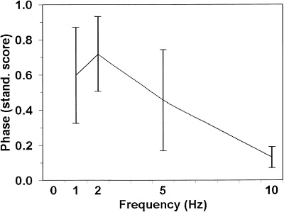
Amplitude of the EROS activity at 80 ms after stimulation (grid reversal) for each frequency stimulation condition. The error bars indicate standard errors of the mean.

Slow Effect (NIRS)

The time course of the slow effect (i.e., the change in DC intensity across the entire block) for each of the four frequency stimulation conditions is presented in Figure 5. The data reported in this figure refer to the locations showing the maximum EROS (fast) response. The data indicate that the amount of light reaching the detector (DC intensity) increases after the onset of stimulation. This was quantified by measuring the average light intensity between second 8 and second 18 of the recording epoch (i.e., second 4–14 of the stimulation period), and comparing it with the period before the onset of stimulation. The increase in DC intensity (on average, 0.29%) was significant, t(7) = 3.19, P < .01, one‐tailed. The data also suggest that this increase takes several seconds after the beginning of stimulation to reach an asymptotic level. We modeled the growth of this curve by fitting a negatively accelerated exponential function to the first 10 sec of recording after the beginning of stimulation. The time constant of this curve was 3.3 sec. The fit of this curve to the observed data was good, r = .982, P < .001. The slow rise of the DC intensity is consistent with the interpretation that it is a reflection of hemodynamic changes, and in particular of an increased blood flow in active cortical areas causing a decrement in the concentration of deoxy‐hemoglobin (the main absorber at the wavelength used in the study). Note that we recorded optical data only up to the time at which the stimulation period ended, and therefore we did not expect the slow response to show a return to baseline within the recording epoch. This choice was determined by limitations in the software that was used for recording the optical data. However, other investigators have previously measured slow optical responses and determined that it does in fact return to baseline after the end of stimulation [see Villringer and Chance, 1997, for a review].

Figure 5.

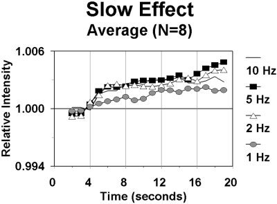
Relative changes in intensity of the light transmitted between source and detector during a block, for each of the four stimulation frequency conditions, averaged across subjects. The grid appeared at time 0, and began reversing after 4 sec.

Figure 5 also suggests that the amplitude of the slow response varies with the stimulation frequency. In particular, the response appears smaller in the 1‐Hz stimulation condition than in the other stimulation conditions. However, this difference did not reach statistical significance, t(7) = 1.83, P < .06, one‐tailed. The amplitude of the slow response (measured as the average DC intensity between second 8 and second 18 divided by the prestimulation baseline) as a function of stimulation frequency is plotted in Figure 6. In this figure the amplitude of the response between second 4 and second 6 (first 2 sec of stimulation), averaged across conditions, is also plotted as an estimate of the baseline‐shift effects (because of the presentation of the stationary grid at the beginning of the block or to other factors, see Methods section). This condition is labeled “0” frequency in the figure. Note that the pattern of slow optical effects presented in this figure indicates an increment of the hemodynamic response up to 5‐Hz stimulation frequency, and a drop for the 10‐Hz stimulation condition. These data roughly replicate those presented by Fox and Raichle [1985] using PET, as well as those of other investigators using the BOLD‐fMRI response [Rees et al., 1997].

Figure 6.

Amplitude of the slow optical response for each stimulation condition. The error bars indicate standard errors of the mean.

Comparison of Fast and Slow Responses

We carried out two types of comparisons between the fast and slow responses. The purpose of these comparisons was to test whether there is a linear relationship between neuronal and hemodynamic activity, at least in medial occipital areas. We used the following linear model of the relationship between neuronal and hemodynamic responses:

where: S is the amplitude of the slow response (average DC Intensity from second 8 to second 18 relative to the baseline level); H is the stimulation frequency (in Hz); F is the amplitude of the fast (EROS) response, measured as the amplitude of the phase delay 80 ms after stimulation compared to the baseline level; and k is a proportionality constant. The application of this model to the grand average results is presented in Figure 7. Note that the abscissa in this graph represents the integrated amplitude of the fast optical response over stimulations, computed on the basis of the model presented above. As a consequence, the order of the amplitude of the fast effects changes with respect to those presented in Figure 3. In the same figure we also traced the regression function associated with the model. The figure indicates that the model represents a good fit for the data. The correlation between the product of the stimulation frequency by the fast effect and the slow effect was r = .981 (P < .01).

Figure 7.

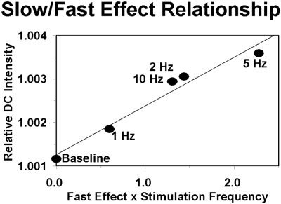
Relationship between the integrated neuronal (EROS) effect (abscissa) and slow hemodynamic (NIRS‐like) effect (ordinate) for each of the four stimulation frequency and for the baseline level (relative DC intensity at the time of beginning of the grid reversals).

The second comparison involved the respective surface distributions of the fast and slow responses. The purpose of this comparison was to test whether the fast and slow response colocalize. We aligned the maps of the surface distributions of the fast effects in different subjects so that the peak of activity was always located in the same pixel (the pixel chosen was the closest to the average location of the peak). This analysis was carried out independently for left and right hemisphere data. The average map obtained in this fashion is represented in the left panel of Figure 8, superimposed over a representative surface cortex image. Then, we realigned the map of the slow effect using, for each subject, the same landmarks used for the fast response (i.e., the slow response was aligned on the basis of the localization of the fast response). The results are shown in the right panel of Figure 8. Areas in red and yellow indicate locations with increased values (i.e., increases in phase for the fast response and increases in intensity for the slow response) with respect to baseline levels, which are typically associated with activation of the corresponding areas; areas in blue indicate locations with decreased values (i.e., decreases in phase for the fast response and decreases in intensity for the slow response) with respect to baseline levels. The significance of these decrements is not yet well understood, although an intriguing possibility is that they may be related to regions of inhibition. In each hemisphere, the location of the maximum slow response corresponded to the location of the maximum fast response. For each hemisphere, the probability of such an occurrence on the basis of chance alone was P = 1/16 = . 0625. The combined probability of this occurring for both hemispheres is P = .0625² = .0039. Thus the data support the claim that the slow response is maximum at the same location were the fast response is maximum (i.e., the two responses colocalize).

Figure 8.

Maps of the neuronal (EROS) and hemodynamic (NIRS‐like) optical responses projected on a representative example of the cortical surface. Areas in red indicate maximum increase in phase delay (EROS map, left) and maximum increase in the light reaching the detector (NIRS‐like map, right)—these types of responses should be considered indices of “increased” activity in these cortical areas. Areas in blue indicate responses in the opposite direction.

Visual Evoked Potentials

The grand average VEP was computed for each electrode location and frequency condition. Because electric fields spread to the whole scalp, it is difficult to determine which particular electrode location should be compared to the optical data. One approach we have used previously is to consider summary measures of the variability across electrode locations as a mean to infer indirectly the occurrence of electrical activity within the brain [Gratton et al., 1997]. Therefore the standard deviations of the voltage activity recorded at different locations was computed for each data point (the data were previously filtered using a five‐points moving average) and frequency condition. These variability measures, expressed as the logarithm of the ratio of the standard deviation for each data point with respect to the variability during a 50‐ms prestimulus period, are presented in Figure 9. For each frequency condition, the variability across electrodes peaked at a latency of 75–80 ms (presumably corresponding to the N75 component of the VEP), corresponding to the time of peak of the EROS response. The amplitude of the brain activity (estimated in this fashion) is considerably smaller in the 10‐Hz condition with respect to the other conditions. We then compared the estimates of the amplitude of the neuronal response at a latency of 80 ms obtained with EROS with those obtained with the VEP (averaged across subjects according to the procedure described above). The correlation between the two measures was r = .96, P < .05. The correlation of the estimate of integrated neuronal activity (i.e., response amplitude × stimulation frequency) obtained with VEP and the estimate of the neurovascular effect obtained with optical measures (see above) was r = .95, P < .05.

Figure 9.

Time course of the VEP for each stimulation frequency condition. The VEP is evaluated in terms of the time course of the variability between electrode locations. Variability is expressed as the log ratio between the standard deviation of the voltage values obtained at different locations at any particular data point and the standard deviation of the voltage values between location observed during the baseline period (the baseline value was not subtracted before this analysis).

The electrical estimates of brain activity obtained in this fashion may be influenced by activity from other areas of the cortex besides medial occipital areas. Therefore we also evaluated the magnitude of the VEP by using a dipole‐modeling approach in which we fitted the observed data with a dipole located in medial occipital cortex. In particular, we modeled the scalp potentials observed a latency of 80 ms (for each frequency condition) by means of a radial dipole located in medial occipital areas, in a location approximately corresponding to the average location of the EROS peak response at this latency (see above). Note that the location and orientation of this dipole were determined a priori (i.e., on the basis of external criteria) and fixed across conditions. This dipole accounted on average for .54 of the total variance (range: .43–.68). This relatively low level of accounted variance is consistent with the idea that other brain areas are also active at this latency. The magnitude of this dipole was approximately the same in the 1‐Hz (.030 arbitrary units), 2‐Hz (.029 units), and 5‐Hz (.029 units) stimulation conditions, but sharply declined in the 10‐Hz condition (.015 units). We used these values as estimates of the magnitude of the average electric field generated in medial occipital cortex in response to each visual stimulation. We then compared these estimates with the optical estimates of neuronal activity in medial occipital cortex. The correlation between these two measures was r = .91, P < .05. The correlation of the integrated estimate of neuronal activity over time obtained using this dipole model approach and the estimates of the hemodynamic response was r = .85, P < .05.

The comparisons of EROS and the VEPs provide additional support to the hypothesis that (a) EROS provides valid quantitative measures of neuronal activity (at least to the extent that VEPs do), and (b) neuronal and hemodynamic measures of responses to visual stimulation in occipital areas are linearly related to each other.

DISCUSSION

The main purpose of the present study was to investigate the relationship between neuronal and hemodynamic measures. In particular, the observation of a linear relationship between the amplitude of the neuronal measure integrated over time and the amplitude of the hemodynamic measure can be used to justify the use of hemodynamic methods to study neuronal activity. Further, the idea that the hemodynamic measure is colocalized with the neuronal measure can be used to justify the use of hemodynamic methods to localize areas of the brain where neuronal activity occurs. Although several studies have reported indirect data in support of these assumptions (at least in the case of high‐contrast visual stimuli) [see Buchel et al., 1998; Buckner et al., 1996; Dale and Buckner, 1997], that work had not involved direct comparisons between measures of neuronal and hemodynamic activity.

A unique feature of the study reported here is the use of optical measures. Optical measures are particularly useful because they are simultaneously sensitive to neuronal and hemodynamic events [Gratton and Fabiani, 1998]. This makes a direct comparison between the two easier to accomplish. A particular advantage of optical measures is that both neuronal and vascular measures refer to approximately the same area of the brain. This is in contrast with comparisons between hemodynamic and electrophysiological measures, which are inherently difficult to colocalize spatially and temporally [see, e.g., Martinez et al., 1999]. Another advantage of optical (with respect to electrophysiological) measures of neuronal activity is that they are largely independent of the organization and geometry of the neurons responsible for the observed effect, a property that is shared with the hemodynamic measures.

As already mentioned, a significant limitation of the study is that our optical instrument only used light of one wavelength. This makes it impossible to distinguish the contributions of changes in oxy‐ and deoxy‐hemoglobin (as well as scattering) to the slow effects observed. The measure obtained for the slow effect can only be taken as a summary measure, reflecting both changes in blood flow and in oxygenation. As optical recording devices using multiple wavelengths (and therefore able to separate different components of the hemodynamic signal) are available (although not in our lab), our results need to be considered preliminary, and further work in this area is needed. Note, however, that the slow effects observed in the present study are largely consistent (in terms of time course and relationship with stimulation frequency) with measures of hemodynamic effects reported in the literature [see Fox and Raichle, 1985]. Note also that an event‐related analysis was used for the fast response but not for the slow response. In fact, the design used in the present study does not permit us to compute an event‐related slow response. The issue of the relationship between fast and slow responses both measured in event‐related designs should be investigated in the future, given the great impact of this type of design in fMRI research.

As expected, the major difference between the neuronal and hemodynamic optical measures appears to be their time course. In fact, the DC‐intensity measure exhibits a time course with a relatively slow onset with respect to the onset of the stimulation period (reaching an asymptotic level only several seconds after stimulation), in a manner consistent with the interpretation that this signal reflects hemodynamic phenomena and, in particular, vasodilation and increased blood flow [Villringer and Chance, 1997]. This contrasts with the time course of the phase delay signal, which shows a rapid increment peaking 60–80 ms after stimulation (i.e., reversal), in a manner consistent with the latency of electrophysiological responses. This different time course provides support for the idea that the DC‐intensity changes do measure hemodynamic events whereas the phase delay changes measure neuronal events. Further support for the neuronal origin of the EROS effect comes from its comparison with the VEP. The two measures peak at the same latency and show a good correspondence in their sensitivity to the experimental manipulation (stimulation frequency).

The results of this study indicate that, at least for the occipital areas under investigation, the hemodynamic signal is linearly related to the integrated neuronal signal. The linear model fits the data, and indicates that the decrement of the slow effect at very high stimulation frequency can be predicted by the substantial decrement of the neuronal response at these high stimulation frequencies. Thus, this experiment provides the first example of a quantitative study of the relationship between neuronal and vascular measures in humans. In addition, the data indicate that the location of maximum hemodynamic response is the same as that of the maximum neuronal response.

Although these data provide support for the use of quantitative analysis of neuroimaging data in the study of neuronal events, it is also clear that a generalization of the findings may be premature. In fact, the relationship between neuronal and hemodynamic responses may vary depending on the region of the brain that is investigated or the type of measure used to quantify the neuronal or hemodynamic effects. Whereas a linear relationship between stimulation frequency and hemodynamic response has been reported for high‐contrast stimuli in occipital areas with both PET blood flow and BOLD‐fMRI measures [Rees et al., 1998; Fox and Raichle, 1985], the relationship may be more complex for temporal areas or for low contrast visual stimuli in visual areas [Rees et al., 1997] in which substantial departures from linearity have been reported. Further, it is possible that the particular procedure used to derive the hemodynamic measure (e.g., the MR‐pulse sequence) may also influence the degree to which additivity is observed. Therefore, although the present results can be considered encouraging, a more extensive evaluation of the issue is needed before the conclusions can be generalized to other areas. Finally, the observation of a linear relationship within the frequency range studied here does not preclude the possibility that more complex functions may also fit the data under other stimulation conditions.

In conclusion, this study reports an initial investigation of the quantitative relationship between noninvasive neuronal and hemodynamic measures as a function of the frequency of visual stimulation. The study exploited the fact that optical methods can be used to provide simultaneous measures of neuronal and hemodynamic activity from (approximately) the same region of the brain. The data indicate that, at least in human medial occipital cortex, the hemodynamic response is linearly related to the integration of the neuronal activity over time.

REFERENCES

- Adachi Usami E (1981): Human visual system modulation transfer function measured by evoked potentials. Neurosci Lett 23: 43–47. [PubMed] [Google Scholar]
- Allison T, Wood CC, McCarthy G (1986): The central nervous system In: Coles MGH, Porges SW, Donchin E, editors. Psychophysiology: systems, processes, and applications. New York: Guilford, pp. 5–25. [Google Scholar]
- Barinaga M (1997): New imaging methods provide a better view into the brain [news]. Science 276: 1974–1976. [DOI] [PubMed] [Google Scholar]
- Belliveau JW, Kennedy DN Jr., McKinstry RC, Buchbinder BR, Weisskoff RM, Cohen MS, Vevea JM, Brady TJ, Rosen BR (1991): Functional mapping of the human visual cortex by magnetic resonance imaging. Science 254: 716–719. [DOI] [PubMed] [Google Scholar]
- Bonhoeffer T, Grinvald A (1996): Optical imaging based on intrinsic signals In: Toga AW, Mazziotta JC, editors. Brain mapping. The methods. San Diego: Academic Press, pp. 55–97. [Google Scholar]
- Buchel C, Holmes AP, Rees G, Friston KJ (1998): Characterizing stimulus‐response functions using nonlinear regressors in parametric fMRI experiments. Neuroimage 8: 140–148. [DOI] [PubMed] [Google Scholar]
- Buckner RL, Bandettini PA, O'Craven KM, Savoy RL, Petersen SE, Raichle ME, Rosen BR (1996): Detection of cortical activation during averaged single trials of a cognitive task using functional magnetic resonance imaging. Proc Natl Acad Sci USA 93: 14878–14883. [DOI] [PMC free article] [PubMed] [Google Scholar]
- Chance B, Kang K, He L, Weng J, Sevick E (1993): Highly sensitive object location in tissue models with linear in‐phase and anti‐phase multi‐element optical arrays in one and two dimensions [published erratum appears in Proc Natl Acad Sci USA 92:4074]. Proc Natl Acad Sci USA 90: 3423–3427. [DOI] [PMC free article] [PubMed] [Google Scholar]
- Cherry SR, Phelps ME (1996): Imaging brain function with positron emission tomography In: Toga W, Mazziotta JC, editors. Brain mapping. The methods. San Diego: Academic Press, pp. 191–222. [Google Scholar]
- Churchland PS, Sejnowski TJ (1988): Perspectives in cognitive neuroscience. Science 242: 741–745. [DOI] [PubMed] [Google Scholar]
- Cope M, Delpy DT (1988): System for long‐term measurement of cerebral blood and tissue oxygenation of newborn infants by near infra‐red transillumination. Med Biol Eng Comput 26: 289–294. [DOI] [PubMed] [Google Scholar]
- Dale AM, Buckner RL (1997): Selective averaging of rapidly presented individual trials using fMRI. Hum Brain Mapp 5: 329–340. [DOI] [PubMed] [Google Scholar]
- DeSoto MC, Fabiani M, Geary D, Gratton G (2001): When in doubt, do it both ways: brain evidence of the simultaneous activation of conflicting responses in a spatial Stroop task. J Cogn Neurosci vol. 13. [DOI] [PubMed] [Google Scholar]
- Fabiani M, Gratton G, Corballis PM (1996): Non‐invasive NIR optical imaging of human brain function with sub‐second temporal resolution. J Biomed Optics 1: 387–398. [DOI] [PubMed] [Google Scholar]
- Fox PT, Raichle ME (1985): Stimulus rate determines regional brain blood flow in striate cortex. Ann Neurol 17: 303–305. [DOI] [PubMed] [Google Scholar]
- Frostig RD, Lieke EE, Ts'o DY, Grinvald A (1990): Cortical functional architecture and local coupling between neuronal activity and the microcirculation revealed by in vivo high‐resolution optical imaging of intrinsic signals. Proc Natl Acad Sci 87: 6082–6086. [DOI] [PMC free article] [PubMed] [Google Scholar]
- Goodman MR, Bauer RM, Corballis PM, Hood DC, Gratton G (1996): Human optical signals and visual evoked potentials (VEPs) from different cone systems. Invest Ophtalmol Vis Sci 37: S708. [Google Scholar]
- Gratton G (1997): Attention and probability effects in the human occipital cortex: an optical imaging study. Neuroreport 8: 1749–1753. [DOI] [PubMed] [Google Scholar]
- Gratton G, Coles MGH, Donchin E (1983): A new method for off‐line removal of ocular artifact. Electroencephalogr Clin Neurophysiol 55: 468–484. [DOI] [PubMed] [Google Scholar]
- Gratton G, Corballis PM (1995): Removing the heart from the brain: compensation for the pulse artifact in photon migration signal. Psychophysiology 32: 292–299. [DOI] [PubMed] [Google Scholar]
- Gratton G, Corballis PM, Cho E, Fabiani M, Hood DC (1995a): Shades of gray matter: noninvasive optical images of human brain responses during visual stimulation. Psychophysiology 32: 505–509. [DOI] [PubMed] [Google Scholar]
- Gratton G, Fabiani M (1998): Dynamic brain imaging: event‐related optical signal (EROS) measures of the time course and localization of cognitive‐related activity. Psychonom Bull Rev. 5: 535–563. [Google Scholar]
- Gratton G, Fabiani M, Corballis PM, Hood D, Goodman MR, Hirsch J, Kim K, Friedman D, Gratton E (1997): Non‐invasive optical measures of localized neuronal activity in the human occipital cortex. Neuroimage 6: 168–180. [DOI] [PubMed] [Google Scholar]
- Gratton G, Fabiani M, Friedman D, Franceschini MA, Fantini S, Corballis P, Gratton E (1995b): Rapid changes of optical parameters in the human brain during a tapping task. J Cogn Neurosci 7: 446–456. [DOI] [PubMed] [Google Scholar]
- Gratton G, Fabiani M, Goodman‐Wood MR, DeSoto MC (1998): Memory‐driven processing in human medial occipital cortex: an event‐related optical signal (EROS) study. Psychophysiology 35: 348–351. [DOI] [PubMed] [Google Scholar]
- Gratton G, Maier JS, Fabiani M, Mantulin WW, Gratton E (1994): Feasibility of intracranial near‐infrared optical scanning. Psychophysiology 31: 211–215. [DOI] [PubMed] [Google Scholar]
- Gratton G, Sarno AJ, Maclin E, Corballis PM, Fabiani M (2000): Toward non‐invasive 3‐D imaging of the time course of cortical activity: Investigation of the depth of the event‐related optical signal (EROS). Neuroimage 11: 491–504. [DOI] [PubMed] [Google Scholar]
- Grinvald A, Lieke E, Frostig RD, Gilbert CD, Wiesel TN (1986): Functional architecture of cortex revealed by optical imaging of intrinsic signals. Nature 324: 361–364. [DOI] [PubMed] [Google Scholar]
- Hoshi Y, Tamura M (1993): Dynamic multichannel near‐infrared optical imaging of human brain activity. J App Physiol 75: 1842–1846. [DOI] [PubMed] [Google Scholar]
- Kato T, Kamei A, Takashima S, Ozaki T (1993): Human visual cortical function during photic stimulation monitoring by means of near‐infrared spectroscopy. J Cereb Blood Flow Metab 13: 516–520. [DOI] [PubMed] [Google Scholar]
- Kwong KK, Belliveau JW, Chesler DA, Goldberg IE, Weisskoff RM, Poncelet BP, Kennedy DN, Hoppel BE, Cohen MS, Turner R, Cheng H‐M, Brady TJ, Rosen BR (1992): Dynamic magnetic resonance imaging of human brain activity during primary sensory stimulation. Proc Natl Acad Sci USA 89: 5675–5679. [DOI] [PMC free article] [PubMed] [Google Scholar]
- Maier J, Dagnelie G, Spekreijse H, van Dijk BW (1987): Principal components analysis for source localization of VEPs in man. Vis Res 27: 165–177. [DOI] [PubMed] [Google Scholar]
- Malonek D, Grinvald A (1996): Interactions between electrical activity and cortical microcirculation revealed by imaging spectroscopy: implications for functional brain mapping. Science 272: 551–554. [DOI] [PubMed] [Google Scholar]
- Martinez A, Anllo‐Vento L, Sereno MI, Frank LR, Buxton RB, Dubowitz DJ, Wong EC, Hinrichs H, Heinze HJ, Hillyard SA (1999): Involvement of striate and extrastriate visual cortical areas in spatial attention. Nat Neurosci 2: 364–369. [DOI] [PubMed] [Google Scholar]
- Mayhew JE, Askew S, Zheng Y, Porrill J, Westby GW, Redgrave P, Rector DM, Harper RM (1996): Cerebral vasomotion: a 0.1‐Hz oscillation in reflected light imaging of neural activity. Neuroimage 4: 183–193. [DOI] [PubMed] [Google Scholar]
- Ogawa S, Tank DW, Menon R, Ellermann JM, Kim SG, Merkle H, Ugurbil K (1992): Intrinsic signal changes accompanying sensory stimulation: functional brain mapping with magnetic resonance imaging. Proc Natl Acad Sci USA 89: 5951–5955. [DOI] [PMC free article] [PubMed] [Google Scholar]
- Okada E, Firbank M, Schweiger M, Arridge SR, Cope M, Delpy DT (1997): Theoretical and experimental investigation of near‐infrared light propagation in a model of the adult head. App Opt 36: 21–31. [DOI] [PubMed] [Google Scholar]
- Papillo JF, Shapiro D (1990): The cardiovascular system In: Cacioppo JT, Tassinary LG, editors. Principles of psychophysiology: physical, social, and inferential elements. Cambridge: Cambridge University Press, pp. 456–512. [Google Scholar]
- Pascual‐Marqui RD, Michel CM, Lehmann D (1994): Low resolution electromagnetic tomography: a new method for localizing electrical activity in the brain. Intl J Psychophysiol 18: 49–65. [DOI] [PubMed] [Google Scholar]
- Rector DM, Poe GR, Kristensen MP, Harper RM (1997): Light scattering changes follow evoked potentials from hippocampal Schaeffer collateral stimulation. J Neurophysiol 78: 1707–1713. [DOI] [PubMed] [Google Scholar]
- Rector DM, Poe GR, Kristensen MP, Harper RM (1995): Imaging the dorsal hippocampus: light reflectance relationships to electroencephalographic patterns during sleep. Brain Res 696: 151–160. [DOI] [PubMed] [Google Scholar]
- Rees G, Howseman A, Josephs O, Frith CD, Friston KJ, Frackowiak RS, Turner R (1997): Characterizing the relationship between BOLD contrast and regional cerebral blood flow measurements by varying the stimulus presentation rate. Neuroimage 6: 270–278. [DOI] [PubMed] [Google Scholar]
- Regan D (1972): Evoked potentials in psychology, sensory physiology, and clinical medicine. New York: Wiley. [Google Scholar]
- Rinne T, Gratton G, Fabiani M, Cowan N, Maclin E, Stinard A, Sinkkonen J, Alho K, Näätänen R (1999): Scalp‐recorded optical signals make sound processing from the auditory cortex visible. Neuroimage 10: 620–624. [DOI] [PubMed] [Google Scholar]
- Tamura M, Hoshi Y, Okada F (1997): Localized near‐infrared spectroscopy and functional optical imaging of brain activity. Philos Trans R Soc Lond B Biol Sci 352: 737–742. [DOI] [PMC free article] [PubMed] [Google Scholar]
- Turner R (1995): Functional mapping of the human brain with magnetic resonance imaging. Semin Neurosci 7: 179–194. [Google Scholar]
- Van der Tweel LH, Verduyn Lunel HFE (1965): Human visual responses to sinusoidally modulated light. Electroencephalogr Clin Neurophysiol 18: 587–598. [DOI] [PubMed] [Google Scholar]
- Villringer A, Chance B (1997): Non‐invasive optical spectroscopy and imaging of human brain function. Trends Neurosci 20: 435–442. [DOI] [PubMed] [Google Scholar]
- Villringer A, Dirnagl U (1995): Coupling of brain activity and cerebral blood flow: basis of functional neuroimaging. Cerebrovasc Brain Metab Rev 7: 240–276. [PubMed] [Google Scholar]
- Wolf U, Wolf M, Toronov V, Michalos A, Paunescu LA, Gratton E (2000): Detecting cerebral functional slow and fast signals by frequency‐domain near‐infrared spectroscopy using two different sensors. OSA Biomedical Topical Meeting 2000, Technical Digest, 427–429. [Google Scholar]