Functional analysis of the periphery effect in human building related areas

Abstract

Several studies have shown that a region in the anterior collateral sulcus (CoS) and a region in the vicinity of the transverse occipital sulcus (TOS) are preferentially activated by images of buildings and scenes. We have found recently that these regions show a strong activation bias to stimuli located in the peripheral visual field. We explore in detail the source of this “periphery” effect. Our results show that the periphery effect can be generated by a large single object occupying the peripheral visual field as well as by multiple small peripheral objects. We also investigated whether the periphery effect was related to the annular shape used in conventional mapping of the visual field periphery and found that the mere presence of a stimulus in the visual field periphery, regardless of object shape, is sufficient to enhance activation. We also found that a small bias toward the peripheral visual field was shown even when the stimulated areas in the central and peripheral parts of the visual field are equated. Finally, our results demonstrate that the periphery effect shows object selectivity that can be obtained even with face images, which are the non‐optimal stimulus for this region. In summary, our study shows that the building‐related CoS and TOS manifest a true but graded retinotopic bias toward the peripheral visual field. Hum. Brain Mapp. 22:17–28, 2004. © 2004 Wiley‐Liss, Inc.

INTRODUCTION

The introduction of functional magnetic resonance imaging (fMRI) of high‐order human visual areas has revealed an elaborate, complex constellation of object‐related regions in the non‐retinotopic occipitotemporal cortex, centered on the lateral occipital complex (LOC) [e.g., Grill‐Spector et al.,2001; Grill‐Spector,2003; Hasson et al.,2003]. A series of studies have demonstrated a striking differential selectivity along the ventral surface of the temporal lobe. While the lateral aspect of the posterior fusiform gyrus (pFs) manifests preferential activation to face images in a region known as the Fusiform Face Area (FFA) [Halgren et al.,1999; Haxby et al.,1999; Kanwisher et al.,1997; McCarthy et al.,1997; Puce et al.,1995], the collateral sulcus (CoS) and the parahippocampal place area (PPA) show preferential activation to buildings and scenes [Aguirre et al.,1998; Epstein and Kanwisher,1998; Haxby et al.,1999] (e.g., Fig. 1). Such high‐order object areas were considered to be largely non‐retinotopic, because they show greatly reduced sensitivity to visual field location of the stimuli. For example, LOC regions show robust activation even to ipsilateral visual field stimulation, something that is absent in early visual areas [Grill‐Spector et al.,1998; Halgren et al.,1999; Tootell et al.,1998].

Figure 1.

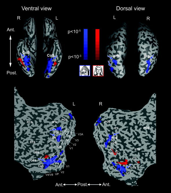
Building‐related regions in a representative subject. Building‐related regions (blue) presented on an inflated (top) and flattened (bottom) brain formats of a single subject. Building‐related regions were defined in a localizer experiment by contrasting activation to building and face images. Preferential activation to faces compared to buildings (red) is shown for comparison. Blue arrows show the ROIs on which subsequent analysis was carried out. Color scales indicate the significance of the statistical test. The inflated brain is shown in ventral (left) and dorsal (right) views. Dotted lines on the left flattened hemisphere denote borders between areas V1, V2, VP, V3, V3A, V4/V8 and MT, which are marked by white arrows. The CoS ROI was defined as the region showing preferential activation to buildings in the vicinity of the CoS, anterior to V4/V8. An additional region was located in the vicinity of the TOS and LOS, anterior to V3A. L, left; R, right; Ant, anterior; Post, posterior; CoS, collateral sulcus; IPS, intraparietal sulcus; ITS, inferior temporal sulcus; POS, parietooccipital sulcus; LOS, lateral occipital sulcus; OTS, occipitotemporal sulcus; PCS, postcentral sulcus; STS, superior temporal sulcus; TOS, transverse occipital sulcus.

We recently found that some retinotopic dimension does seem to be preserved in these areas, as visual field eccentricity is represented differentially in the face compared to building‐related regions. We have found that building‐related regions show a significantly greater activation to peripheral stimulation compared to face‐related regions [Levy et al.,2001]. More specifically, in the building‐related CoS, activation was higher to a peripheral ring containing multiple enlarged object copies compared to a centrally located single object (e.g., Fig. 2a). A similar result was obtained recently in a dorsal region in the vicinity of the TOS, which also exhibits a preference to building stimuli [Hasson et al.,2003]. These results raise several questions regarding the nature of the periphery effect. First, it is of interest to find whether the effect, similar to the general activity in the CoS and the TOS, is object selective, i.e., whether it is stronger for a certain class of objects compared to others. Specifically, we tested whether the periphery effect is different for optimal versus non‐optimal categories. Second, the observed periphery effect may be attributed to several alternative factors. One option is that the enhanced activation may not necessarily be due to the peripheral location of the stimuli, but rather to the annular shape that is conventionally used in the peripheral stimuli. Alternatively, because the peripheral ring included a number of repeating objects, it could be that activation in the CoS and the TOS simply reflects the number of objects presented rather than their peripheral location.

Figure 2.

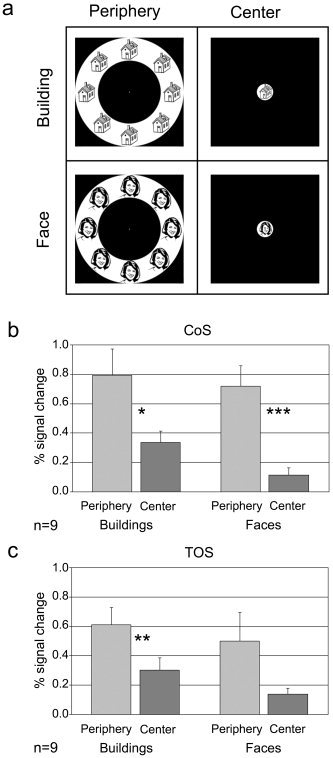
Experiment 1. Mapping the periphery effect using a single object category. a: Examples of stimuli used in Experiment 1. Line drawings of faces and buildings were shown either in the center of the visual field or in multiple enlarged copies in a peripheral ring. Subjects were instructed to fixate on a central dot. b: Percent signal change measured in the CoS building‐related region. A peripheral effect was obtained for both faces and buildings. c: The same effect was obtained in the TOS building‐related region. Asterisks, significant difference in a one‐tailed t‐test (*P < 0.05, **P < 0.005, ***P < 0.001).

Finally, it could be that the observed peripheral bias was due actually to the enlarged area of visual field stimulation used to compensate for the magnification factor, rather than the visual field location, i.e., the activation may be directly proportional to the area of retinal stimulation. We report several results relevant to these aspects. Our study shows that the periphery effect is indeed related to the visual field periphery, and can be explained best as reflecting a process of large‐scale integration across the visual field.

SUBJECTS AND METHODS

Subjects

In total, 21 subjects participated in one or more of the experiments (13 women; age range, 20–52 years). Data of one subject were discarded due to problems in data acquisition and data of another subject were discarded due to excessive head motion. Of the remaining 19 subjects, 11 participated in Experiment 1, 5 in Experiment 2, and 8 in Experiment 3. Of these, one subject participated in all three experiments, three participated in two experiments, and the rest in a single experiment. Building‐related areas were localized in a separate experiment in 17 subjects and borders of retinotopic areas were delineated in 15 of those subjects All subjects had normal or corrected‐to‐normal vision and provided written informed consent. The Tel‐Aviv Sourasky Medical Center approved the experimental protocol.

MRI Setup

Subjects were scanned on a 1.5T Signa Horizon LX 8.25 GE scanner equipped with a quadrature surface coil (Nova Medical Inc., Wakefield, MA), which covered the posterior brain regions. Blood oxygenation level‐dependent (BOLD) contrast was obtained with gradient‐echo echo‐planar imaging (EPI) sequence (TR = 3,000 msec, TE = 55 msec, flip angle = 90 degrees, field of view 24 × 24 cm², matrix size 80 × 80). The scanned volume included 17 nearly‐axial slices of 4‐mm thickness and 1‐mm gap. A whole‐brain spoiled gradient (SPGR) sequence was acquired on each subject to allow accurate cortical segmentation, reconstruction, and volume‐based statistical analysis. T1‐weighted high resolution (1.1 × 1.1 mm) anatomic images of the same orientation as the EPI slices were also acquired to facilitate the incorporation of the functional data into the 3‐D space.

Stimuli

Stimuli were generated on a PC, projected via an LCD projector (Epson MP 7200) onto a tangent screen positioned over the subject's forehead, and viewed through a tilted mirror.

Experimental Design

All three experiments started with a blank period of 21 sec and ended with a 15‐sec blank period, during which a uniform gray screen and a fixation point were presented. The experiments were short‐block designed. Each block lasted 9 sec and consisted of nine images of the same type. Blocks were pseudo‐randomly ordered and interleaved with 6‐sec blank periods.

Experiment 1

This experiment was aimed at testing whether the periphery effect is object‐selective. The experiment consisted of six conditions: three categories × two eccentricities. Black and white line drawings of faces and buildings as well as character strings (reported elsewhere [Hasson et al.,2002]) were shown either in the center of the visual field (diameter: 3 degrees) or in a peripheral ring (inner diameter: 11.5 degrees, outer diameter: 20 degrees), which contained eight enlarged copies of the same stimulus. Sixteen different images of each type were used. Each image was presented for 200 msec, followed by an 800‐msec blank. Each condition was repeated four times, except for the character conditions, which were repeated eight times each. Subjects were instructed to fixate on a red dot positioned at the center of the screen throughout the experiment.

Experiment 2

This experiment was aimed at distinguishing between the effects of peripheral location and multiplicity of objects. The experiment consisted of four conditions. Two conditions consisted of black and white line drawings of buildings, shown either in a small ring at the center of the visual field (inner diameter: 0.8 degrees, outer diameter: 3.3 degrees, “central building”) or enlarged to fill a peripheral region (inner diameter: 5 degrees, outer diameter: 20 degrees, “peripheral building”). Note that the stimuli in the peripheral building condition were identical to those in the central building condition, except for their size, including a blank hole in the center of all stimuli (Fig. 3a). Two additional conditions contained black and white line drawings of faces (“medium face”) and buildings (“medium building”), subtending 12 × 12 degrees. In the central building and peripheral building conditions 72 different images of each type were used. In the medium face and medium building conditions, 27 different images of each type were used. Each image was presented for 250 msec, followed by a 750‐msec blank. The first two conditions were repeated eight times, and the last two conditions were repeated six times. Subjects covertly carried out a sequential matching task (1‐back) while fixating on a red dot presented throughout the experiment.

Figure 3.

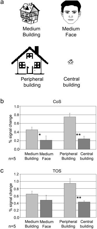
Experiment 2. Mapping eccentricity using a single object stimulus. a: Examples of stimuli used in Experiment 2. Stimuli were line drawings of buildings shown either in the center (central building) or enlarged to fill the periphery (peripheral building). Peripheral stimuli were identical to central ones and differed only in size. Line drawings of faces and buildings of an intermediate size were also shown (medium face and medium building). Subjects carried out a 1‐back task while maintaining central fixation. b: Percent signal change measured in the CoS building‐related region. As expected, this region exhibited preferential activation to buildings compared to faces. Importantly, a peripheral effect was obtained even though the peripheral stimulus contained a single object. c: A similar trend was observed in the TOS region. Asterisks, significant difference in a one‐tailed t‐test (*P < 0.05, **P < 0.01).

Experiment 3

This experiment was aimed at differentiating between the effects of the peripheral location of the stimulus and the visual field it covers. The experiment consisted of eight conditions: two categories × four combinations of eccentricity and size. Multiple copies of gray‐level drawings of buildings and manmade objects (tools, cars and chairs) were shown in a ring in one of four sizes/eccentricities (Fig. 4): 10 copies in a ring whose diameters were 2.5–8 degrees (“logarithmic mid”), 10 enlarged copies in a ring whose diameters were 8–20 degrees (“logarithmic periphery”), 20 copies in a ring whose diameters were 2.5–14 degrees (“Euclidean mid”), and 20 copies of the same size in a ring whose diameters were 14–20 degrees (“Euclidean periphery”). We could thus compare activation to stimuli that differed both in eccentricity and in area (logarithmic periphery vs. logarithmic mid) or to stimuli that differed in eccentricity but covered a similar area (Euclidean periphery vs. Euclidean mid). Eighteen different images of each type were used. Each image was presented for 200 msec, followed by an 800‐msec blank. The first visual epoch in the experiments consisted of geometrical patterns and was modeled as a separate predictor in the statistical analysis. Subjects were instructed to fixate on a red dot presented throughout the experiment.

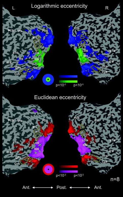
Figure 4.

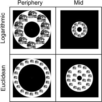
Experiment 3. Euclidean vs. logarithmic eccentricity mapping. Examples of stimuli used in Experiment 3. Stimuli were drawings of buildings and objects shown in four different locations. Logarithmic periphery and logarithmic mid stimuli were used to map the peripheral effect similar to previous experiments (logarithmic eccentricity). Equal‐sized Euclidean periphery and Euclidean mid stimuli were used to measure the net peripheral effect due to peripheral location and not to stimulus size (Euclidean eccentricity). Subjects were instructed to fixate a central dot.

Building Localizer

Building‐related regions were localized using an external block‐designed localizer [Hasson et al.,2003]. Subjects were presented with images of buildings and faces (and two other conditions: common objects and patterns not used here). Each condition lasted 9 sec and was repeated four times (one subject), seven times (15 subjects) or eight times (one subject). Images were presented for a short duration (150–800 msec), followed by a blank period. Epochs were pseudo‐randomly ordered and interleaved with 6‐sec blanks. Subjects had to covertly carry out a 1‐back task (16 subjects) or a recognition task (one subject) while fixating on a red dot.

Mapping Borders of Visual Areas

The representations of vertical and horizontal visual field meridians were mapped in 15 subjects to delineate borders of retinotopic areas [DeYoe et al.,1996; Engel et al.,1994; Sereno et al.,1995]. Stimuli were presented in 18‐sec blocks, interleaved with 6‐sec blank periods. Images were presented for 250 msec in a consecutive manner. Stimuli consisted of triangular wedges that were presented either vertically (upper or lower vertical meridians) or horizontally (left or right horizontal meridians). Each condition was repeated four times. Two versions of the experiment were run. In the first, the wedges consisted of either gray‐level natural images or black and white objects from texture pictures [Grill‐Spector et al.,1998]. In the second, the wedges consisted of colored copies of objects superimposed on colored textures. Subjects were instructed to fixate on a small central cross.

Data Analysis

fMRI data were analyzed with the BrainVoyager software package (R. Goebel, Brain Innovation, Masstricht, The Netherlands) and with complementary in‐house software. The first three images of each functional scan were discarded. The functional images were superimposed on 2D anatomic images and incorporated into the 3‐D data sets through trilinear interpolation. The complete data set was transformed into Talairach space [Talairach and Tournoux,1988]. Preprocessing of functional scans included 3‐D motion correction and filtering out of low frequencies up to 5 cycles per experiment in Experiment 2 and 10 cycles per experiment in all other experiments. No spatial smoothing was applied to the data. The cortical surface was reconstructed from the 3‐D SPGR scan. The procedure included segmentation of the white matter using a grow‐region function, the smooth covering of a sphere around the segmented region, and the expansion of the reconstructed white matter into the gray matter. The surface was then unfolded, cut along the calcarine sulcus and flattened. Statistical analysis was conducted on the flattened cortex.

Statistical Analysis

Building‐related regions were identified in each subject using the building localizer experiment. Statistical analysis was based on the General Linear Model [Friston et al.,1995]. A box‐car predictor, assuming a 3‐sec hemodynamic lag, was constructed for each experimental condition except blank, and the model was independently fitted to the signal of each voxel. A coefficient was calculated for each predictor using a least‐squares algorithm. A t‐test contrasting the coefficient of the building predictor with that of the face predictor was conducted, and regions of interest (ROIs) were defined as clusters of at least six contiguous functional voxels in which the P value of the test was less than 0.05 and which lay anteriorly to the retinotopic areas. In two subjects for which we did not map the retinotopic borders, the ROIs were defined as the most anterior part of the activated area (starting at 4 cm from the posterior edge of the flattened hemisphere in the CoS and 3 cm in the vicinity of the TOS).

In Experiments 1–3 we sampled the time‐course in each ROI and computed the percent signal change compared to the blank period preceding it. Repetitions of each condition and all time points in each condition were then averaged. Finally, results were averaged across subjects.

In Experiment 3, additional ROIs were defined as regions showing a periphery effect in the CoS and the TOS, by contrasting the predictors of the logarithmic periphery and the logarithmic mid conditions (Fig. 4). The time course of the Euclidean periphery and Euclidean mid conditions, which were not included in the statistical test, was sampled and averaged as explained above.

Periphery Bias Index

In Experiment 1, a periphery bias was calculated for each object category in each ROI of each subject. The periphery bias was defined as (periphery − center)/(periphery + center), where periphery and center are the percent signal changes compared to blank in the periphery and center, respectively, averaged across the time points in each epoch and the repetitions of each condition. A periphery bias of 1 reflects a total preference for the peripheral visual field, whereas a value of 0 reflects equal activation to the central and peripheral visual fields.

Multi‐Subject Analysis

In the multi‐subject analysis, time courses of all subjects were converted into Talairach space and z‐normalized. The multi‐subject maps (Fig. 5) were obtained using a random effect procedure [Friston et al.,1999] and the maps were projected on a flattened Talairach normalized brain.

Figure 5.

Euclidean vs. logarithmic eccentricity mapping: activation maps. The periphery effect was obtained using stimuli that were magnified compared to the more central stimuli (top) and using stimuli that were equal in size (bottom). Most of the CoS building‐related region (yellow contours) was within the periphery‐biased area, except for the most anterior tip. Color scales indicate the significance of the statistical test. TOS, transverse‐occipital sulcus; other abbreviations as in Figure 1.

Statistical Significance

Calculation of significance values in the activation maps (Fig. 1 and 5) was based on the individual voxel significance and on the minimum cluster size of six voxels [Forman et al.,1995]. The probability of a false positive was determined from the frequency count of cluster sizes within the entire cortical surface, using a Monte Carlo simulation.

RESULTS

Localizing Building‐Related Regions

Building‐related regions were identified using an external localizer by contrasting the activation to building and face images. The obtained active regions that lay anteriorly to retinotopic areas were defined as ROIs and subsequent analysis was confined to them. In all 17 subjects, building‐related activation was obtained in the ventral occipitotemporal cortex (VOT) in the vicinity of the CoS. In 15 subjects this activation was bilateral, in one subject it was confined to the right hemisphere, and in another to the left hemisphere (Table I). Figure 1 shows the location of the building‐related CoS in a typical case on an inflated brain in a ventral view and on a flattened brain. This region corresponds to the building‐related region described by Aguirre et al. [1998] and extends into the parahippocampal place area (PPA) described by Epstein and Kanwisher [1998]. Building‐related activation was also obtained in the dorsal occipitotemporal cortex (DOT) in the vicinity of the transverse occipital sulcus (TOS), extending in some cases to the intraparietal sulcus (IPS) and the lateral occipital sulcus (LOS), in agreement with previous results [Hasson et al.,2003; Haxby et al.,1999]. A typical example can be seen in Figure 1 on an inflated brain in a dorsal view and on a flattened brain. Such activation was found in 14 subjects, bilaterally in 13 subjects and in the right hemisphere of one subject (Table I), but was weaker and more variable than the CoS activation.

Table 1.

Talairach coordinates of building‐related regions

Region	Left hemisphere					Right hemisphere
	n	Volume (cm3)	x	y	z	n	Volume (cm3)	x	y	z
Experiment 1
CoS (VOT)	9	0.7 ± 0.4	−24 ± 2	−44 ± 4	−9 ± 2	9	0.8 ± 0.4	22 ± 2	−44 ± 5	−9 ± 2
TOS (DOT)	8	0.9 ± 0.3	−35 ± 6	−78 ± 3	12 ± 5	9	0.7 ± 0.4	32 ± 5	−76 ± 4	15 ± 5
Experiment 2
CoS (VOT)	5	0.7 ± 0.6	−26 ± 1	−43 ± 3	−9 ± 1	5	0.8 ± 0.5	25 ± 1	−39 ± 2	−9 ± 2
TOS (DOT)	5	0.9 ± 0.4	−33 ± 3	−78 ± 3	16 ± 6	5	0.7 ± 0.3	33 ± 3	−77 ± 5	13 ± 3
Experiment 3
CoS (VOT)	7	0.6 ± 0.4	−26 ± 3	−41 ± 6	−9 ± 1	7	0.8 ± 0.5	23 ± 2	−41 ± 6	−8 ± 4
TOS (DOT)	5	0.7 ± 0.5	−32 ± 2	−81 ± 2	14 ± 7	5	0.7 ± 0.4	31 ± 2	−77 ± 3	20 ± 6

Talairach coordinate values are mean ± SD in mm.

CoS, anterior collateral sulcus; VOT, ventral occipitotemporal cortex; TOS, transverse occipital sulcus; DOT, ventral occipitotemporal cortex.

Experiment 1: Mapping the Periphery Effect With a Single Category

The basic periphery effect reported previously in the CoS was obtained using a mixture of different objects [Levy et al.,2001]. The first question we addressed here was whether the periphery effect is category dependent. In Experiment 1, we thus used face and building images, shown either in the center or in a peripheral ring [Fig. 2a, see also Hasson et al.,2002]. As expected, this region manifested a clear preferential activation to building images compared to face images (building center vs. face center, P < 0.02, one‐tailed t‐test, n = 9) and a clear bias toward the peripheral ring of objects compared to the central object stimulus (Fig. 2b). Importantly, this peripheral bias was obtained for both object categories (building periphery vs. building center, P < 0.05; face periphery vs. face center, P < 0.001). In fact, face images showed a slightly stronger periphery bias compared to that produced by building images, despite the fact that they were suboptimal stimuli when presented at the center (face periphery bias, 0.8 ± 0.1 [mean ± SEM]; building periphery bias, 0.3 ± 0.2; face periphery bias vs. building periphery bias, P = 0.07, two‐tailed t‐test). The source of the periphery effect for faces seemed to be the substantial reduction in building selectivity when the object images were presented in the peripheral location. Although a slight bias toward building stimuli was observed, it did not reach significance (building periphery vs. face periphery, P = 0.14).

Similar results were obtained in the TOS (Fig. 2c). This region exhibited a preferential activation to buildings when presented in the center (building center vs. face center, P < 0.02, n = 9), but not in the periphery (building periphery vs. face periphery, P = 0.18) and also showed a periphery bias, which was significant in the case of buildings and approached significance in the case of faces (building periphery vs. building center, P < 0.005; face periphery vs. face center, P = 0.05).

Experiment 2: A Single Peripheral Object

In Experiment 1, the peripheral stimuli consisted of rings containing multiple objects; therefore, the peripheral effect may have been due to the increased number of objects in the periphery or to the ring‐like arrangement typical of eccentricity‐mapping stimuli. To explore these possibilities we conducted Experiment 2. In this experiment, we enlarged single building images shown in the center of the visual field (Fig. 3a, Central building) so that they impinged on the visual field periphery (Fig. 3a, Peripheral building). The enlarged building images were identical in shape and features to the central ones. In two additional conditions, subjects were presented with middle‐sized images of other buildings and faces (Fig. 3a, Medium building and Medium face).

The results, averaged across five subjects, show that the periphery effect in the CoS was preserved when the peripheral stimulus was a single enlarged building (Fig. 3b, peripheral building vs. central building, P < 0.01, one‐tailed t‐test, n = 5). As expected, this region also exhibited preferential activation to buildings compared to faces (medium building vs. medium face, P < 0.05). The activation to these middle‐sized buildings was in‐between the activation to the central and peripheral buildings (central building, 0.24 ± 0.06%; medium building, 0.45 ± 0.06%; peripheral building, 0.75 ± 0.09%). A similar peripheral bias was observed in the TOS (Fig. 3c, peripheral building vs. central building, P < 0.01, n = 5). We thus conclude that the periphery effect was not due to a difference in the shape or number of object stimuli presented.

Experiment 3: Effect of Peripheral Location Versus Large Area of Stimulation

The results of Experiment 2 were also compatible with the possibility that the peripheral effect was due to the larger area covered by the peripheral stimuli, rather than their peripheral visual field location. In early visual areas, the visual field is represented in a log‐polar manner, i.e., the representation of the center of the field is magnified compared to its periphery. Standard eccentricity mapping experiments compensate for the lower magnification factor in the periphery by enlarging the peripheral stimuli. The same manipulation was used in Experiments 1 and 2; however, this experimental design confounds peripheral location with a larger stimulation area. It could be that the peripheral effect observed in the CoS is in fact a result of the larger area occupied by the peripheral stimuli compared to the mid or central ones.

To explore this possibility, we conducted Experiment 3. The experiment enabled us to carry out two comparisons. First, we could compare activation to stimuli that differed both in their eccentricity and in the extent of area they covered, similar to previous experiments (Fig. 4, top). We term this mapping logarithmic eccentricity. In addition, we could compare activation to stimuli that had equal stimulation areas but differed in their maximal eccentricity (Fig. 4, bottom). We term this mapping Euclidean eccentricity. If the peripheral effect was due exclusively to the larger overall stimulated area covered by the peripheral stimuli, then we would expect similar activation levels to stimuli presented in different locations, provided that their areas were identical. In each condition, separate epochs contained either building or object images, but because there was no significant difference in the percent signal change between these conditions (two‐way ANOVA, main factors: category and location; interaction, CoS: P = 0.9; TOS: P = 0.88), we averaged the results across category.

Figure 5 shows the average eccentricity maps obtained in a group of eight subjects. The top map was created by contrasting activation to the small mid‐eccentricity ring with activation to the magnified peripheral one (logarithmic eccentricity), as was done in previous experiments. The bottom map was created by contrasting activation to the equal‐sized mid and periphery rings (Euclidean eccentricity). Superimposed on the maps are the contours of building‐related activations in the localizer experiment averaged across the same subjects.

Importantly, in posterior low‐tier areas, a clear center periphery map was obtained in both comparisons, indicating that subjects indeed maintained fixation. As expected, in these areas, equating the size of the stimuli enlarged the cortical area responding to the mid stimuli and reduced the area responding to the peripheral ones. Also as expected, most of the CoS building‐related region (yellow contours) was activated preferentially by the peripheral stimuli when the periphery was enlarged compared to the mid‐stimulation. Critically, however, the same peripheral bias was observed even when the total areas of the mid and peripheral stimuli were equated.

Sampling the building‐related regions yielded a periphery effect both in the CoS and in the TOS when the peripheral stimuli were magnified (logarithmic eccentricity, periphery vs. mid, CoS: P < 0.05, n = 8; TOS: P < 0.05, n = 5). Comparison of activation to stimuli that differed only in their location revealed a trend toward the periphery that was close to significance in the CoS (Euclidean eccentricity, periphery vs. mid, P = 0.08, n = 8) but not in the TOS (P = 0.12, n = 5). We reported previously [Levy et al.,2001] that the most anterior tip of the building‐related region may be outside of the periphery‐biased area. To avoid mixing such non‐peripheral regions, we conducted another analysis, in which only voxels showing the conventional (logarithmic) periphery effect, which lay anteriorly to retinotopic areas in the CoS and TOS, were examined (Fig. 6). Our results show that these voxels manifested a significant bias toward the visual field periphery even when stimuli were equated in their stimulated area, both in the CoS (periphery vs. mid, P < 0.0005, one‐tailed t‐test, n = 6) and in the TOS (P < 0.05, n = 5). It thus seems that the periphery effect in the CoS was due largely to the peripheral location of the stimuli; however, this does not rule out an additional area effect. To test for such an effect, we re‐sampled the data, this time localizing voxels showing either a logarithmic or a Euclidean periphery bias (logarithmic periphery + Euclidean periphery vs. logarithmic mid + Euclidean mid). This enabled us to compare activation to the logarithmic vs. Euclidean periphery conditions, which were identical in their extreme eccentricity but differed in the area they covered. The comparison revealed a significantly higher activation to the logarithmic periphery (P < 0.05, one‐tailed t‐test, n = 6) in the CoS and a similar, albeit not significant, trend in the TOS (P = 0.1, one‐tailed t‐test, n = 5). An area effect thus seems to exist in building‐related areas, in addition to the true periphery effect.

Figure 6.

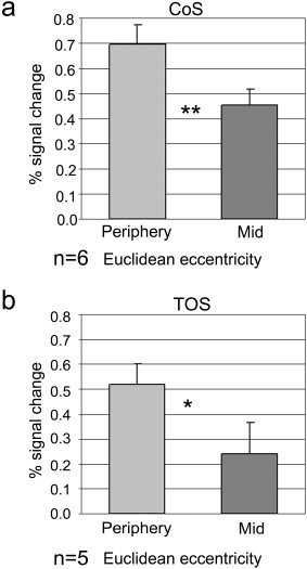
Euclidean eccentricity mapping: time course analysis. Percent signal change in response to the equal‐size stimuli, measured in voxels that exhibited a bias toward the enlarged periphery in the CoS (a) and the TOS (b) anterior to retinotopic areas. The peripheral effect in these voxels was preserved even though the area covered by the stimuli was equated. Asterisks, significant difference in a one‐tailed t‐test (*P < 0.05, **P < 0.0005).

DISCUSSION

The Nature of the Peripheral Effect in the CoS

The results of Experiment 1 show that the periphery effect of the CoS was not specific to stimuli that preferentially activated the CoS, such as buildings, but could be obtained even using faces, which hardly activated this region when presented centrally. A likely explanation for this result seems to be the marked reduction in category selectivity for peripheral stimuli observed in the CoS. The CoS thus showed higher selectivity to building images when these images were presented centrally compared to when they were presented peripherally, although in terms of overall activation, the peripheral stimuli produced a higher activation level. The source of this differential selectivity is not clear. One possibility may be an interaction with the neighboring fusiform gyrus, so that the high activation to faces presented centrally in this region is causing the reduction in face activation in the CoS via some sort of lateral inhibition process. Additional tests, however, will be required to clarify the mechanisms underlying this finding.

Experiment 2 ruled out the possibility that the periphery effect was due to the number of objects presented or the ring shape of the conventional peripheral stimulus. In this experiment, unlike conventional eccentricity mapping experiments, the peripheral stimuli were constructed by enlarging a single central object. In terms of shape, the central and peripheral stimuli shared the exact same features and differed only in their size, yet the periphery effect was maintained. These results are compatible with a previous study [Epstein and Kanwisher,1998], which failed to find preferential activation to multiple objects compared to a single object in the PPA unless these objects were arranged in a spatial context.

The result of Experiment 2 cannot be interpreted as produced by a sharply localized retinotopic effect, similar to early visual areas, because the increase in activation when moving from central building stimuli to middle‐sized ones and then to peripheral ones was gradual (Fig. 3b). A clear‐cut outcome of Experiment 2 is thus the finding of a gradual size effect in the CoS, by which larger objects produced higher activation than did smaller ones.

The size effect in the CoS in this experiment, however, might be due either to the stimuli impinging on more peripheral visual field locations, or purely due to the larger area of the visual stimuli.

Experiment 3 was designed to differentiate between these two alternatives, and its results indicate that a large fraction of the effect, at least for mid to peripheral locations, was a true peripheral bias. Thus, even when the area of stimulation was equated, stimuli in more peripheral locations still caused a preferential activation (Fig. 6). This could mean that a single object in some part of the peripheral visual field is enough to activate the CoS. Results of a recent study [Epstein et al.,2003], however, show that at least in the PPA this is not the case: two small objects in the periphery did not activate this region more than a single object in the center. In addition, we found that enlarging the area of the stimulus also increased activation in the region. It thus seems that visual stimulation occupying a large part of the visual field and spanning a wide range of polar angles is needed to activate the region.

The results of Experiment 3 also provide further confirmation of the finding that the number of objects included in the stimuli was not critical for activation, because the same number of objects was used in the peripheral and mid stimuli (Fig. 4, bottom).

The results could not be explained by differential eye movement patterns, because clear center periphery maps were obtained in early retinotopic areas (e.g., see Figure 5 for Experiment 3; similar maps were obtained in Experiments 1 and 2). Such clearly demarcated eccentricity maps provide an intrinsic control, which indicates that subjects did not deviate from fixation, because due to the high foveal magnification, such deviations would have resulted in substantial blurring of boundaries of the foveal/peripheral representations.

Implications for the Center Periphery Organization

How are the present results related to the center periphery organization? Several lines of evidence suggest that qualitatively different processes take place in the center‐biased pFs and the periphery‐biased CoS and PPA. A number of studies have implicated the pFs in object recognition. Whether it contains a module, specialized for face recognition [Kanwisher,2000] or an area of expertise, which can be trained to specialize in other objects [Gauthier et al.,2000], it seems that the pFs singles out for detailed analyses specific objects of interest embedded in the visual scene. This is compatible with the center bias found in this region, which implies higher resolution than that of the CoS. This high resolution enables fine analysis of visual information, leading to extraction of objects or features matching some templates that are represented in this region. This is not to say that the pFs deals primarily with local features. On the contrary, several studies have shown that the response of this region is more holistic than feature based [e.g., Hasson et al.,2001; Kourtzi and Kanwisher,2001]. The PPA, on the other hand, has been shown to deal with the overall layout of the visual environment: it was highly activated by outdoor scenes, even more than by buildings [Epstein and Kanwisher,1998] and seems to be sensitive to the relative positioning of visual elements within a scene. For example, the PPA was more activated by intact room images than by images that were fractured and rearranged, and by scenes containing no objects compared to those containing objects with no spatial context [Epstein and Kanwisher,1998]. This notion of sensitivity to global spatial arrangement was emphasized by the recent finding that the representation in the PPA is viewpoint specific [Epstein et al.,2003], i.e., sensitive to changes in the spatial relationship between the scene and the observer.

The peripheral effect found in the CoS is compatible with a role in navigation and representation of the visual environment. Navigation entails integration and comparison of information across the visual field and the present results are congruent with such long‐distance “comparator” processes. Activation in the CoS thus increased as the stimulus became more peripheral, even if the area it covered remained the same, and it also increased when the stimulus was enlarged, even if it did not reach farther eccentricities (Experiment 3). In addition, the peripheral effect did not depend on multiplicity of objects, but was associated with any kind of complex visual information (Experiment 2). It seems that the maximal eccentricity of the stimulus determines the level of CoS activation, which makes sense if comparison of information across large distances in the visual field is required. The fact that the periphery effect remained for faces as well, however, may imply that the CoS has a more general role in spatial integration. This role may be required for navigation but can also be used in other tasks.

The region in the CoS that was the basis of analysis in these studies may not be identical to the PPA described by Epstein and Kanwisher [1998]. It could be that scene images activate a slightly more medial region compared to that activated by building images, and that this medial region is less responsive to other objects even when presented in the peripheral field.

Further support for the notion that spatial integration is highly emphasized in peripheral stimuli comes from a recent study that explored the phenomenon of reduced acuity caused by clutter of stimuli in the periphery, known as “crowding” [Parkes et al.,2001]. This study demonstrated that even when clutter of stimuli in the periphery prevented subjects from estimating the orientation of individual stimuli, they could still estimate the average orientation precisely, proving that they had access to information that was integrated across the field.

The difference between the pFs and the CoS does not necessarily imply the existence of segregated modules. It is compatible with both a modular organization [Spiridon and Kanwisher,2002] and a distributed one [Avidan et al.,2002; Haxby et al.,2001]. The pFs and CoS could either be two distinct entities carrying out different processes or two extremes of one continuum that starts with high resolution and fine analysis and ends with low resolution and global synthesis.

The Periphery Effect in Dorsal Occipitotemporal Cortex

The ventral building‐related region in the CoS is mirrored by a dorsal region in the vicinity of the TOS that shows preferential activation to buildings compared to faces and common objects [Hasson et al.,2003]. It remains unclear, however, how these areas differ functionally. The preference for buildings does not necessarily mean that the region is selective to buildings. It could be that this region shows preferential activation to additional object categories, or alternatively that both the CoS and TOS regions are selective to buildings but each carries out a different process. For example, it could be that TOS is an intermediate region between the ventral stream, the activation of which is related to stimulus appearance, and the dorsal stream, which deals with stimulus position [Aguirre and D'Esposito,1997]. Further research will be needed to define the properties of this region more precisely.

CONCLUSIONS

The periphery effect found in the building‐related region in the CoS shows a true but graded bias toward the visual field periphery, rather than a preference of multiple objects or a large stimulation area. The effect was obtained for optimal as well as non‐optimal stimuli.

REFERENCES

- Aguirre GK, D'Esposito M (1997): Environmental knowledge is subserved by separable dorsal/ventral neural areas. J Neurosci 17: 2512–2518. [DOI] [PMC free article] [PubMed] [Google Scholar]
- Aguirre GK, Zarahn E, D'Esposito M (1998): An area within human ventral cortex sensitive to “building” stimuli: evidence and implications. Neuron 21: 373–383. [DOI] [PubMed] [Google Scholar]
- Avidan G, Hasson U, Hendler T, Zohary U, Malach R (2002): Analysis of the neuronal selectivity underlying low fMRI signals. Curr Biol 12: 964–972. [DOI] [PubMed] [Google Scholar]
- DeYoe EA, Carman GJ, Bandettini P, Glickman S, Wieser J, Cox R, Miller D, Neitz J (1996): Mapping striate and extrastriate visual areas in human cerebral cortex. Proc Natl Acad Sci USA 93: 2382–2386. [DOI] [PMC free article] [PubMed] [Google Scholar]
- Engel SA, Rumelhart DE, Wandell BA, Lee AT, Glover GH, Chichilnisky EJ, Shadlen MN (1994): fMRI of human visual cortex. Nature 369: 525. [DOI] [PubMed] [Google Scholar]
- Epstein R, Graham KS, Downing PE (2003): Viewpoint‐specific scene representations in human parahippocampal cortex. Neuron 37: 865–876. [DOI] [PubMed] [Google Scholar]
- Epstein R, Kanwisher N (1998): A cortical representation of the local visual environment. Nature 392: 598–601. [DOI] [PubMed] [Google Scholar]
- Forman SD, Cohen JD, Fitzgerald M, Eddy WF, Mintun MA, Noll DC (1995): Improved assessment of significant activation in functional magnetic resonance‐imaging (fMRI)—use of a cluster‐size threshold. Magn Reson Med 33: 636–647. [DOI] [PubMed] [Google Scholar]
- Friston J, Homes A, Worsley K, Poline J, Frith C, Frackwowiak R (1995): Statistical parametric maps in functional imaging: a general linear approach. Hum Brain Mapp 2: 189–210. [Google Scholar]
- Friston KJ, Holmes AP, Price CJ, Buchel C, Worsley KJ (1999): Multisubject fMRI studies and conjunction analyses. Neuroimage 10: 385–396. [DOI] [PubMed] [Google Scholar]
- Gauthier I, Skudlarski P, Gore JC, Anderson AW (2000): Expertise for cars and birds recruits brain areas involved in face recognition. Nat Neurosci 3: 191–197. [DOI] [PubMed] [Google Scholar]
- Grill‐Spector K (2003): The neural basis of object perception. Curr Opin Neurobiol 13: 159–166. [DOI] [PubMed] [Google Scholar]
- Grill‐Spector K, Kourtzi Z, Kanwisher N (2001): The lateral occipital complex and its role in object recognition. Vision Res 41: 1409–1422. [DOI] [PubMed] [Google Scholar]
- Grill‐Spector K, Kushnir T, Hendler T, Edelman S, Itzchak Y, Malach R (1998): A sequence of object‐processing stages revealed by fMRI in the human occipital lobe. Hum Brain Mapp 6: 316–328. [DOI] [PMC free article] [PubMed] [Google Scholar]
- Halgren E, Dale AM, Sereno MI, Tootell RB, Marinkovic K, Rosen BR (1999): Location of human face‐selective cortex with respect to retinotopic areas. Hum Brain Mapp 7: 29–37. [DOI] [PMC free article] [PubMed] [Google Scholar]
- Hasson U, Harel M, Levy I, Malach R (2003): Large‐scale mirror‐symmetry organization of human occipito‐temporal object areas. Neuron 37: 1027–1041. [DOI] [PubMed] [Google Scholar]
- Hasson U, Hendler T, Ben Bashat D, Malach R (2001): Vase or face? A neural correlate of shape‐selective grouping processes in the human brain. J Cogn Neurosci 13: 744–753. [DOI] [PubMed] [Google Scholar]
- Hasson U, Levy I, Behrmann M, Hendler T, Malach R (2002): Eccentricity bias as an organizing principle for human high‐order object areas. Neuron 34: 479–490. [DOI] [PubMed] [Google Scholar]
- Haxby JV, Gobbini MI, Furey ML, Ishai A, Schouten JL, Pietrini P (2001): Distributed and overlapping representations of faces and objects in ventral temporal cortex. Science 293: 2425–2430. [DOI] [PubMed] [Google Scholar]
- Haxby JV, Ungerleider LG, Clark VP, Schouten JL, Hoffman EA, Martin A (1999): The effect of face inversion on activity in human neural systems for face and object perception. Neuron 22: 189–199. [DOI] [PubMed] [Google Scholar]
- Kanwisher N (2000): Domain specificity in face perception. Nat Neurosci 3: 759–763. [DOI] [PubMed] [Google Scholar]
- Kanwisher N, McDermott J, Chun MM (1997): The fusiform face area: a module in human extrastriate cortex specialized for face perception. J Neurosci 17: 4302–4311. [DOI] [PMC free article] [PubMed] [Google Scholar]
- Kourtzi Z, Kanwisher N (2001): Representation of perceived object shape by the human lateral occipital complex. Science 293: 1506–1509. [DOI] [PubMed] [Google Scholar]
- Levy I, Hasson U, Avidan G, Hendler T, Malach R (2001): Center‐periphery organization of human object areas. Nat Neurosci 4: 533–539. [DOI] [PubMed] [Google Scholar]
- McCarthy G, Puce A, Gore JC, Allison T (1997): Face specific processing in the human fusiform gyrus. J Cogn Neurosci 9: 605–610. [DOI] [PubMed] [Google Scholar]
- Parkes L, Lund J, Angelucci A, Solomon JA, Morgan M (2001): Compulsory averaging of crowded orientation signals in human vision. Nat Neurosci 4: 739–744. [DOI] [PubMed] [Google Scholar]
- Puce A, Allison T, Gore JC, McCarthy G (1995): Face‐sensitive regions in human extrastriate cortex studied by functional MRI. J Neurophysiol 74: 1192–1199. [DOI] [PubMed] [Google Scholar]
- Sereno MI, Dale AM, Reppas JB, Kwong KK, Belliveau JW, Brady TJ, Rosen BR, Tootell RB (1995): Borders of multiple visual areas in humans revealed by functional magnetic resonance imaging. Science 268: 889–893. [DOI] [PubMed] [Google Scholar]
- Spiridon M, Kanwisher N (2002): How distributed is visual category information in human occipito‐temporal cortex? An fMRI study. Neuron 35: 1157–1165. [DOI] [PubMed] [Google Scholar]
- Talairach J, Tournoux P (1988): Co‐planar stereotaxic atlas of the human brain. New York: Thieme Medical Publishers. [Google Scholar]
- Tootell RB, Mendola JD, Hadjikhani NK, Liu AK, Dale AM (1998): The representation of the ipsilateral visual field in human cerebral cortex. Proc Natl Acad Sci USA 95: 818–824. [DOI] [PMC free article] [PubMed] [Google Scholar]