

Abstract
Holes in the skull may have a large influence on the EEG and ERP. Inverse source modeling techniques such as dipole fitting require an accurate volume conductor model. This model should incorporate holes if present, especially when either a neuronal generator or the electrodes are close to the hole, e.g., in case of a trephine hole in the upper part of the skull. The boundary element method (BEM) is at present the preferred method for inverse computations using a realistic head model, because of its efficiency and availability. Using a simulation approach, we have studied the accuracy of the BEM by comparing it to the analytical solution for a volume conductor without a hole, and to the finite difference method (FDM) for one with a hole. Furthermore, we have evaluated the influence of holes on the results of forward and inverse computations using the BEM. Without a hole and compared to the analytical model, a three‐sphere BEM model was accurate up to 5–10%, while the corresponding FDM model had an error <0.5%. In the presence of a hole, the difference between the BEM and the FDM was, on average, 4% (1.3–11.4%). The FDM turned out to be very accurate if no hole is present. We believe that the difference between the BEM and the FDM represents the inaccuracy of the BEM. This inaccuracy in the BEM is very small compared to the effect that holes can have on the scalp potential (up to 450%). In regard to the large influence of holes on forward and inverse computations, we conclude that holes in the skull can be treated reliably by means of the BEM and should be incorporated in forward and inverse modeling. Hum. Brain Mapping 17:179–192, 2002. © 2002 Wiley‐Liss, Inc.
Keywords: EEG, ERP, inverse modeling, BEM, FDM, skull conductivity
INTRODUCTION
Neuronal activity in the brain can result in macroscopic electrical currents that can be recorded at the scalp as electroencephalogram (EEG) or as event related potentials (ERP). The observed scalp potentials are not only determined by the location and strength of the neuronal generators, but also by the geometry and conductive properties of the head. The skull is known to have a large impact on the resulting scalp potential distribution, which is due to its relative low conductivity compared to the other tissues in the head. We examined the effect of local inhomogeneities in the skull, i.e., holes, on the scalp potential and whether these can be incorporated in the boundary element method (BEM). This can be regarded as a specific example of skull inhomogeneities in general. In principle these can be incorporated using the BEM, but currently these are commonly excluded from volume conduction models for the head.
Holes in the skull can be natural, such as the ear holes or the hole through which the optic nerve passes. Holes also may be present due to unnatural causes like neurosurgery or fractures caused by accidents. In general the tissue in a hole in the skull will have a larger conductivity than that of the skull itself, and therefore it can have a shunting effect between the compartments interior and exterior of the skull. Currents, which normally would be confined mainly to the interior of the skull, can flow through the hole and thereby influence the scalp potential. It has been shown previously that the presence of holes in the skull has indeed a large impact on the scalp potential distribution. In simulation studies the finite element method (FEM) has been used [van den Broek, 1997; van den Broek et al., 1998] as well as the finite difference method (FDM) [van Burik, 1999; Vanrumste, 2001; Vanrumste et al., 2000]. Not only holes, but also the presence of thin sections in the skull, such as at the frontal and temporal base of the skull and in the eye sockets, have shown to have an impact on source localization accuracy [Huiskamp et al., 1999].
Localization of the neuronal generators of EEG and ERP can be carried out by using physical models for the neuronal current source configuration and for the volume conductor. For a small number of focal generators of brain activity, the scalp potential generated by the model sources (usually dipoles) is iteratively computed using a specific volume conduction model. The location and strength of the sources are adapted until the mismatch between the computed model potential and the measured potential is minimal [Scherg and von Cramon, 1985, 1986]. Alternatively, a distributed source model for the generators of the potential distribution can be assumed. This requires a forward computation of the scalp potential generated by each source element. Subsequently the strength of the distributed source is computed by using a linear estimation technique [e.g., Pasqual‐Marqui et al., 1994]. Irrespective of whether a discrete or distributed source model is assumed, inverse computation of the source parameters requires a large number of evaluations of the forward computation of the potential. This imposes a restriction on the inverse techniques: only those methods that are computationally fast in the forward computation are usable for inverse modeling.
Models of the head based on multiple concentric spheres are commonly used for inverse modeling. The analytical expressions for the forward computation of the potential are known for these models [Cuffin and Cohen, 1979; Kavanagh et al., 1978]. These expressions can be evaluated quite efficiently, and even faster approximation techniques for the analytical potential have been developed [Ary et al., 1981; Berg and Scherg, 1994; Sun, 1997]. More accurate computations of the forward potential can be done using a realistically shaped model of the head [Buchner et al., 1995; Leahy et al., 1998; Roth et al., 1997], but this requires a numerical solution to the forward problem. The boundary element method (BEM) is the most popular numerical method for inverse computations with a realistically shaped model of the head. This is largely due to its relatively high computational efficiency compared to the other numerical methods available. In the preparatory phase, the BEM requires a computation of a single matrix that describes the effect of the volume conductor and the computation of the inverse matrix. Once this has been computed, the scalp potential for any given source configuration can be evaluated with little computational cost. This makes the performance of the BEM comparable to that of the analytical spherical head models.
Localizing brain activity on basis of EEG/ERP measurements in the presence of holes in the skull requires that the effects of the hole on the volume conduction are incorporated in the model. At present, the BEM is the only technique enabling the use of realistic head models including holes in the skull, which is fast enough for the large number of iterations required by the inverse methods.
The goal of this study is to assess whether the BEM is accurate enough for forward and inverse modeling in the case of holes in the skull. This goal will be approached in two steps. First, the solutions for volume conductors without a hole in the skull obtained by the finite difference method (FDM) and the boundary element are compared to the analytical solutions. Next, the results obtained by the FDM and the BEM in the presence of a hole in the skull are compared to evaluate the accuracy of the BEM in that situation. The FDM will serve as the “gold standard” in the latter comparison. Finally, the actual effect of holes in the skull on the scalp potential and on inverse computations will be demonstrated for a variety of source and volume conduction model configurations.
MATERIALS AND METHODS
To be able to compute the analytical solution for the potentials for comparison, we make use of a simplified geometry representing the head. This geometry consists of one or three spheres, each with a homogeneous conductivity. The single sphere model has a radius of 100 mm and a conductivity of 1 S/m. The three spheres have radii of 88, 92, and 100 mm (representing the brain, skull and scalp compartment) and a conductivity of 1, 1/80, and 1 S/m, normalized to the conductivity of the brain [Geddes and Baker, 1967]. These conductivities correspond to the values that are normally used in forward and inverse EEG studies. Recent work by Oostendorp et al. [2000] has shed some doubt on the validity of the conductivity ratio of 1/80 for the skull and suggested a higher conductivity (lower resistance). Other recent studies, however, report on values of the skull conductivity around 1/80 of that of the brain and skin tissue [Cuffin, 1993; Gabriel et al., 1996; Law, 1993] and no consensus seems to exist as yet. It can be assumed that the effects of a hole will be greater when the conductivity of the skull is lower, i.e., when there is a larger difference in conductivity of the skull and the hole. In this study we adopted the value of 1/80 for the skull conductivity because it will provide the largest effects and, hence, the strongest test case.
Evaluating the accuracy of the BEM and FDM
To assess the accuracy of the BEM, we have computed the potential for a number of source and volume conduction geometries. We used a one‐ and a three‐sphere volume conduction model with no hole and a three‐sphere model with a hole centered on the positive z‐axis. The diameter of the hole was varied from 10, 20, 30 to 60 mm. The source consisted of a single radial dipole on the z‐axis, which pointed toward the hole. Extensive FEM simulations [van den Broek, 1997] have shown that a dipole pointing toward a hole in the skull causes the largest influence on the surface potential, and we used this finding to guide our simulations. The eccentricity of the dipole was varied from the origin toward the surface with z‐values of 0, 2, 4, 6, and 8 cm (Fig. 1). This configuration with a radial source pointing along the z‐axis and with a hole on the z‐axis has a rotational symmetry around the z‐axis.
Figure 1.
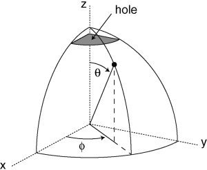
Overview of the Cartesian and spherical coordinate system in one octant, schematically depicting the location of the hole in the skull.
Forward computations of the surface potentials, due to the source on the z‐axis, were made for the one‐ and the three‐sphere geometries with no hole using the BEM and FDM. These were compared to the analytical computed surface potentials, to validate both methods. Subsequently, a hole was created on the z‐axis in the BEM and FDM models, and the potentials were compared to each other to assess the accuracy relative to each other. The relative error (RE) was used to quantify the correspondence between the potentials computed by different methods:
 |
(1) |
In this equation V i is the potential at electrode i computed by one method, ϕi is the computed potential at i by the other method and N is the number of electrodes. The RE was also used to express the difference between the models with and without a hole, in which case it is called the relative difference.
For the comparison between the BEM, the FDM, and the analytical computed potential, we used only those electrode locations that we were able to compute the potential in each method. The electrodes lying in the yz‐plane fully describe the potential for a radial source on the z‐axis due to the rotational symmetry. We used 20 electrodes along a surface contour in this plane, with θ ranging from 0 to 180 degrees (Fig. 1). This resulted in an inter‐electrode distance of 8.3 mm. The electrodes were chosen such that they coincide with vertices of the mesh for the BEM, because this results in a more accurately computed potential for the BEM [Fuchs et al., 2001]. In the comparisons of the potential without a hole, an average reference potential was used in the computation of the RE. When a hole was present in the models, we used a reference electrode located at the bottom of the outermost sphere. By putting the reference as far away as possible from the location of the hole, the referenced potential distribution is influenced as little as possible by the presence or absence of the hole.
Finite difference method
The FDM is based upon the notion that, for source free regions, the divergence of the current density is zero in any volume conductor (quasi‐static approach). This implies that the flux of the current density through any closed surface is zero. This corresponds to Kirchof's law for an equivalent resistive electrical circuit, in which the current going into each node equals the current leaving the node.
Expressing the electric field as function of the potential, the combination with Ohm's law yields
| (2) |
The application of Gauss's law leads to the following surface integral for a surface enclosing a region with a source of magnitude I, corresponding to a monopolar source.
| (3) |
For any surface surrounding a source free region, this surface integral equals zero.
| (4) |
The FDM mesh was constructed by placing nodes on a regular grid in spherical coordinates. Due to the rotational symmetry of the problem, no currents flow in the tangential direction around the z‐axis (Fig. 1). Therefore it suffices to create a mesh consisting only of a single slice of the sphere (Fig. 2A).
Figure 2.
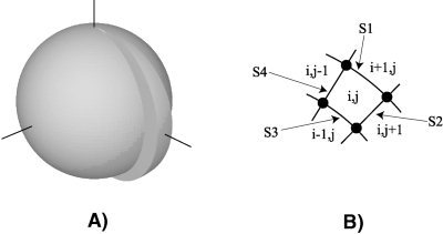
Construction of the mesh used for the FDM. The left shows how a single slice is taken from a sphere, retaining the rotational symmetry around the z‐axis. On the right a single volume element of this slice is shown with the definition of the indices of the volume element (i, j) and the surfaces (S1–S4).
To compute the potential at each node, equations (3) and (4) are evaluated for each node in the mesh. For nodes that are source free, the total current density flux through their surface equals zero. Starting off with a mesh in which all nodes are assumed to be source free gives the following equation for each node:
| (5) |
where ΔS n is the bounding surface of the node at edge n (Fig. 2B). The areas of each of the four bounding surfaces for our configuration are
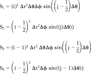 |
(6) |
and the effective conductivity σn for each boundary is set at
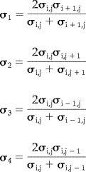 |
(7) |
This results in a single linear equation for each node. Combining these into a linear system of equations gives
| (8) |
where matrix C is sparse with only four non‐zero elements per row and vector b contains a zero for each source free node. Vector ϕ is the unknown potential at each node.
A dipolar source was introduced into the FDM model by putting two monopolar current sources at two adjacent nodes. One node acts as the source with a positive monopole, the other one acts as the sink, with an equally strong but negative monopole. This results in two non‐zero values in vector b. Subsequently, equation (8) was solved for the potential ϕ, which can be efficiently done by exploiting the sparsity of matrix C. We used the default Matlab 5.3 solver for sparse linear systems, which implements Gaussian elimination with partial pivoting [Gilbert et al., 1992]. From the resulting vector containing the potential at all nodes, only the surface nodes were taken. The potentials at the electrode locations were computed using linear interpolation between the surface nodes.
The FDM was applied to a mesh containing 100 nodes in both the radial direction and the tangential direction θ, resulting in a total of 10,000 nodes. In addition, coarser meshes with 50 × 50 nodes and 100 × 50 nodes and finer meshes with 200 × 100 nodes were used in the configurations without a hole. For the configurations with a hole, we used a mesh consisting of 100 × 113 nodes. Using 113 nodes along the tangential direction gives a tangential node distance of 5 mm at the location of the skull, with which the desired hole diameters could be realized.
Boundary element method
The approach used by the BEM is based upon the integral formulation of the forward problem for the electric potential [Barnard et al., 1967a, b]. The volume conductor is assumed to consist of multiple compartments, each with a homogenous and isotropic conductivity. A closed triangular mesh describes the bounding surfaces between the compartments. The potential can be assumed to be constant over the triangles (centre of mass approach) or can be assumed to vary within the triangles as a linear function of the values at the vertices (vertex approach) [de Munck, 1992; Meijs et al., 1989]. The vertex approach is more accurate and computationally faster and therefore the method of our choice. The formulation of the BEM has been described in detail elsewhere [Meijs et al., 1989; Oostendorp and van Oosterom, 1989]. We present only the main result:
| (9) |
This equation shows the separation within the BEM of the volume conduction effect and of the effect that the source has on the surface potential ϕ. Matrix A in this equation depends only on the geometric and conductive properties of the volume conductor. Vector ϕ∞ (the source term) is the infinite medium potential, i.e., the potential on all vertices due to the sources for an infinitely large homogeneously conducting medium. To compute the potential due to any specific (not necessarily dipolar) source, it suffices to compute the infinite medium potential due to that source, followed by the multiplication with the system matrix A. This matrix needs to be calculated only once, which allows for fast repetitive evaluations of the surface potential using the BEM.
The meshes for the BEM were created by starting with an icosahedron (12 vertices), followed by three rounds of triangle refinement in which the triangle‐shape was maintained constant [Bank et al., 1983]. The vertices of the resulting mesh were subsequently scaled toward the desired sphere radius. This results in a regular mesh with 642 vertices and 1,280 triangles. Local refinement of the triangulation was applied in the region near the positive z‐axis, which is both the region where the hole was located, as well as the region to which the more superficial dipoles were close [Yvert et al., 1995, 1996]. Starting with a surface description of the three compartments, a hole in the skull was designed in three different fashions, which are schematically depicted in Figure 3. The three methods (open, dented, and pegged) are described below.
Figure 3.
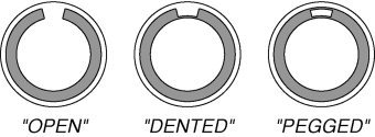
The three methods used to create a hole in the skull for the BEM. From left to right the open, dented, and pegged model are schematically shown. Note that in reality the skull and brain surfaces touch in the dented model and that in the pegged model the compartment representing the hole touches the brain and the skull.
The first method uses a surface description of a skull compartment with a real hole, and we call this an “open” surface. Starting off with intact surface descriptions of brain and the skull, a hole is made in both surfaces by removing the vertices and triangles near the hole. The orientation of the triangles (i.e., surface normals) of the brain surface is inverted, after which the edge of the hole in the brain surface is connected with a strip of new triangles to the edge of the hole in the skull surface. This results in a single closed triangular surface, describing both the outer and the inner surface of the skull (that was previously the outer surface of the brain). The resulting BEM model consists of two surfaces only; one for the skin and the other one is the newly created skull surface. Because the brain and skin compartment are fused through the hole into one compartment, this method can only be used if they have the same conductivity.
In the second method, the vertices of the original skull surface triangulation are locally moved toward the brain surface. This results in a dent in the skull surface similar to the surfaces used by Cuffin [1993], but in our situation the resulting skull thickness was put to zero. We ensured that the vertices and triangles of the skull surface within the hole exactly matched the vertices and triangles of the brain surface, resulting in an exact correspondence of the two surfaces within the hole. The upright edge of the hole in the skull triangulation was re‐triangulated to create a sharp transition from the skull toward the dented hole. In the regions where the two surfaces touch, there is an infinitely thin layer that has the conductivity of the skull. Assuming the same conductivity for the scalp and brain compartments, the corresponding vertices of the brain and skull surfaces will cancel out in the BEM. The resulting BEM model consists of three surfaces just as in the normal situation describing the brain, skull and scalp compartments. The dented description is more flexible than the open description in the respect that it does not require the conductivities of brain and skin to be the same.
The third method uses an additional compartment to describe the hole. The vertices of the skull triangulation overlying the hole are identified, as well as the vertices of the brain triangulation directly underneath the hole. These vertices (and their triangulation) are assimilated into a new surface by connecting the edges of these two surfaces, using a triangle strip. The resulting geometry is similar to a “peg.” By placing this peg between the skull and the brain surface, and specifying a high conductivity similar to that of the brain and skin, effectively a hole in the skull is created. The vertices of the peg or hole compartment were created, to exactly correspond to the brain triangulation on the inside, and to the skull triangulation on the outside. In the regions where the peg touches the other two surfaces, there is an infinitely thin layer having the conductivity of the skull. The “pegged” description offers the flexibility that different conductivities for brain and skin can be used, and a different conductivity for the tissue within the hole is possible.
The “dented” and “pegged” descriptions of the skull consist of interfaces, which touch each other near the hole. The BEM involves the computation of the solid angles of all triangles as seen from all other vertices. The computation of these solid angles is straightforward, except in the case that the observation vertex is part of the triangle. If the vertex and triangle are located at the same interface, we use the Auto Solid Angle (ASL) method [Meijs et al., 1989] to compute the solid angle. In the ASL method, the solid angle of the surface element is computed for an observation point that approaches the surface from within. If the triangle is at another interface than the vertex, but touching the vertex nevertheless, the solid angle is computed for an observation point approaching the surface from without. Because the touching triangle has a vertex, which coincides with the observation vertex, the value for the solid angle can be computed as 4π minus the auto solid angle found for the coinciding vertex.
The presence of a compartment with very low conductivity, such as the skull between the source and the surface electrodes, results in poor computational accuracy for the BEM. This problem can be largely overcome by the use of the Isolated Potential Approach (IPA) [Hämäläinen and Sarvas, 1989]. In the IPA first the potential w 0 at the inner compartment in isolation is computed. Next, the potential at all vertices is computed by using the same equation as equation (1), but with a modified source term, which is a weighted summation of ϕ∞ and w 0 [Hämäläinen and Sarvas, 1989]. Note that the IPA can only be used for the dented and the pegged skull, because for the open geometry no isolated compartment containing the source can be identified. Whether the IPA also improves the accuracy of the potentials computed using the BEM in the case of a skull with holes, is hard to predict. We examined the influence of the IPA on the accuracy of the BEM, by applying it on the three‐sphere configuration without a hole, and by applying it to the “pegged” skull BEM model.
RESULTS
Accuracy of the FDM in case of no hole
FDM potentials were computed for the one‐ and three‐sphere configurations. A radial oriented dipole was placed at z = 0, 2, 4, 6, and 8 cm. The RE of the FDM potentials, compared to the analytical potentials for a single sphere and for three spheres, are presented in Table I. For a single sphere, the coarsest mesh with 50 × 50 nodes already resulted in a small RE of 0.2–1.4%. The quality improved slightly with more nodes, and the finest mesh with 200 × 100 nodes resulted in an error <0.5% for all dipole locations. For a three‐sphere configuration, REs were smaller: the mesh with 50 × 50 nodes resulted in an error <0.2% for each dipole location and the 200 × 100 mesh resulted in errors <0.1%. It can be concluded therefore, that the FDM is very accurate in computing the surface potential for the one‐ and three‐sphere configurations with a radial oriented dipole, regardless of dipole eccentricity.
Table I.
Relative errors of the FDM potential compared to the analytical solution (without a hole)*
| Dipole excentricity (cm) | FDM vs. analytical mesh 50 × 50 | FDM vs. analytical mesh 100 × 50 | FDM vs. analytical mesh 100 × 100 | FDM vs. analytical mesh 200 × 100 |
|---|---|---|---|---|
| Single sphere model | ||||
| 0 | 0.19 | 0.22 | 0.05 | 0.06 |
| 2 | 0.07 | 0.06 | 0.01 | 0.01 |
| 4 | 0.15 | 0.12 | 0.02 | 0.02 |
| 6 | 0.25 | 0.20 | 0.05 | 0.05 |
| 8 | 1.41 | 1.28 | 0.61 | 0.48 |
| Three sphere model | ||||
| 0 | 0.20 | 0.24 | 0.05 | 0.06 |
| 2 | 0.05 | 0.05 | 0.01 | 0.01 |
| 4 | 0.08 | 0.07 | 0.01 | 0.01 |
| 6 | 0.14 | 0.12 | 0.02 | 0.02 |
| 8 | 0.30 | 0.26 | 0.14 | 0.10 |
Values are expressed as %.
The source was a radial dipole located along the z‐axis. The results pertaining to different FMD mesh refinements are shown.
Accuracy of the BEM in case of no hole
Using the BEM and FDM, the potentials generated by a dipole in a one‐sphere model and in a three‐sphere model with no hole, were computed. The reference for the potential was chosen to be the average over all electrodes. The potential was computed for a radial dipole at z = 0, 2, 4, 6, and 8 cm. The RE was used to express the differences between these two numerically computed potentials and the analytical potential.
Comparisons of the BEM to the analytical solution for the one‐ and three‐sphere configurations without a hole are presented in Table II. The main results are as follows: for a single sphere BEM model with 642 evenly distributed vertices, the RE ranged from 0.1% for a dipole in the center to 0.6% for the most superficial dipole location. A three‐sphere BEM model with 642 evenly distributed vertices for each sphere (with a total of 1,926 vertices and 3,840 triangles) resulted in an error of 8–11% when the isolated potential approach was used. Without the isolated potential approach, however, the error was much larger for dipoles near the surface, even up to 190% for the most superficial dipole. The use of a mesh with 1,306, 1,308, and 642 vertices for the brain, skull and scalp surfaces respectively, where the brain and skull surfaces were locally refined near the positive z‐axis (i.e., near the location of the dipole), resulted in a RE of 7% for the central dipole to 4% for the most superficial one when the isolated potential approach was applied (not presented in the table), and 5% (central) to 10% (superficial) when the isolated potential approach was not applied. Irrespective of the use of the isolated potential approach, the accuracy of the BEM in a three‐sphere model was therefore estimated to be 5–10%, when using a properly refined mesh.
Table II.
Relative errors of the BEM potential compared to the analytical solution (without a hole)*
| Dipole excentricity (cm) | Single sphere model BEM vs. analytical | Three sphere model | ||
|---|---|---|---|---|
| BEM vs. analytical without IPA | BEM vs. analytical with IPA | Locally refined BEM without IPA | ||
| 0 | 0.14 | 5.7 | 8.1 | 4.8 |
| 2 | 0.15 | 7.6 | 8.5 | 3.9 |
| 4 | 0.18 | 14.4 | 9.8 | 3.7 |
| 6 | 0.25 | 31.9 | 12.0 | 9.2 |
| 8 | 0.62 | 190.5 | 10.8 | 10.4 |
Values are expressed as %.
The source was a radial dipole located along the z‐axis.
Comparison of BEM and FDM in case of a hole
Because there is no analytical solution available for the computation of the potential for a volume conductor with a hole, we are limited to the comparison between the BEM and FDM in this particular case. We compared the potentials computed with BEM and FDM generated by a radial dipole along the z‐axis of a three‐sphere model with a hole of varying size on the positive z‐axis. The BEM potentials were computed without the application of the isolated potential approach.
Comparing the three different methods of creating a hole in the skull for the BEM with the FDM results shows that the open, dented, and pegged all have a similar RE. Depending on the dipole eccentricity, the open model for a 60‐mm hole has a relative difference ranging from 2.7–8.5%. The dented model has a relative difference of 2.7–5.8% and the pegged model results in 1.9–5.5% difference. Table III lists the total comparisons of the different models. The RE of each model is slightly larger for a dipole near the center, as well as for a dipole near the hole. A dipole halfway from the center toward the hole has the smallest error in each of the BEM models.
Table III.
Relative differences between the FDM and BEM potentials for the different BEM hole models
| Dipole excentricity (cm) | Open model 60‐mm hole | Dented model 60‐mm hole | Pegged model 60‐mm hole |
|---|---|---|---|
| 0 | 7.8 | 5.8 | 5.5 |
| 2 | 4.6 | 4.5 | 4.0 |
| 4 | 2.7 | 2.7 | 1.9 |
| 6 | 8.5 | 3.3 | 4.2 |
| 8 | 5.6 | 4.6 | 4.9 |
Values are expressed as %.
Based on the comparisons between the methods to create a hole for the BEM, the pegged hole model was selected for further study. Table IV lists the results for the different hole sizes and dipole locations. The RE between the FDM and BEM ranges from 2.8–5.0% for the 10‐mm hole, up to 1.3–11.4% for the 30‐mm hole. The BEM potentials for the largest hole (60 mm) are again more similar to the FDM, with differences of 4.0–5.5%. Although the differences between FDM and BEM may appear rather large, they should be seen with respect to the actual change in scalp potentials, due to the presence of a hole. These are orders of magnitude larger, and range from 5% for a central dipole with the smallest hole up to over 400% for a superficial dipole with a large hole. The comparisons between the potential distributions without and with a hole are presented in more detail in a next section.
Table IV.
Relative differences between the FDM and BEM potentials in the presence of a hole in the skull of varying diameter
| Dipole excentricity (cm) | BEM vs. FDM 10‐mm hole | BEM vs. FDM 20‐mm hole | BEM vs. FDM 30‐mm hole | BEM vs. FDM 60‐mm hole |
|---|---|---|---|---|
| 0 | 5.0 | 4.7 | 3.8 | 5.5 |
| 2 | 3.0 | 2.5 | 1.3 | 4.0 |
| 4 | 2.8 | 2.1 | 3.0 | 1.9 |
| 6 | 5.0 | 1.8 | 5.1 | 4.2 |
| 8 | 3.2 | 1.9 | 11.4 | 4.9 |
Values are expressed as %.
IPA in the presence of a hole in the skull
Previous research has shown that the isolated potential approach increases accuracy [Hämäläinen and Sarvas, 1989; Meijs et al., 1989]. The actual assumption of the source being located in the isolated skull compartment is invalidated, however, when a hole is present in the skull. The comparisons between the BEM and the analytically computed potentials for a closed skull demonstrate that the application of the IPA only increases the accuracy in specific situations. Using a model with three spheres, each triangulated regularly with 642 vertices, the IPA dramatically improves the accuracy for a superficial radial dipole: the RE between BEM and analytical potential reduces from 190 to 10.8%. For a central dipole in combination with a regular triangulation however, the RE increases from 5.7 to 8.1% due to the application of the IPA.
We also compared the BEM potential to the analytical potential for a locally refined mesh. This refined mesh was based on the same refinement used for the models with a hole, simply by leaving out the peg representing the hole. The mesh for the scalp surface was evenly triangulated and the surfaces for the brain and skull were locally refined near the hole. With this mesh, the RE for the most superficial dipole was only 10.4% without the IPA, compared to 3.6% with the IPA. The central dipole again showed the opposite effect: the RE increased from 4.8 to 7.3% by using the IPA.
These results show that the application of the IPA is not always beneficial in the case of a closed skull. It works very well for superficial sources near a relative coarse triangulation of the interior brain and skull surfaces. For deep sources, however, the IPA decreases the accuracy. For superficial sources in combination with a locally refined mesh, the IPA slightly increases the accuracy, but not very much.
Because there is no analytical solution for the potential in the case of a hole available, we cannot make strong statements about the influence of the IPA on the BEM, in case of a hole. Using the FDM solution as reference, however, the accuracy of the BEM in the case of a hole, with and without the IPA, seems comparable, with only differences of a few percent (not presented quantitatively).
Influence of a hole on the forward solution
The previous sections established the accuracy of both the BEM and FDM for forward potential computations in one‐ and three‐sphere volume conductor models without a hole, where the FDM is the most accurate. Furthermore, it was demonstrated that the potentials computed with BEM and FDM in the case of a hole in the skull correspond closely, with a difference from 1.3% to a maximum of 11.4%. For computational reasons the FDM model was limited to a configuration with a rotational symmetry around the z‐axis. In contrast to this, the BEM does not have to be limited to a certain source or volume conductor configuration and therefore we used it in the following computations. The actual effect of the hole on the potential distribution is demonstrated, by comparing potential distributions for three‐sphere volume conductors, with and without a hole for a wide range of source configurations. In these computations we used the IPA, although similar results would have been obtained without it. The main reason to use it is that we wanted to compute the potential both for sources near the hole, as well as for sources near the skull but further away from the hole. For the first sources, the IPA does not make a great deal of difference. For the latter sources, which are near to the non‐refined regions of the skull, the IPA greatly increases accuracy.
The potential was computed on all 642 vertices of the outer surface of the BEM model. The reference for the potential was chosen at the opposite side of the hole, along the negative z‐axis. The effect of a hole of varying diameter on the potential, expressed as the relative difference, is shown in Figure 4 for a dipole moving along the z‐axis from the center of the sphere toward the hole. The left hand side (Fig. 4A) shows the effect for a radial dipole (pointing in the z‐direction toward the hole), the right hand (Fig. 4B) side shows the effect for a tangential dipole. The difference in the potential distribution varies from near zero for a source far away, to over 400% for a radial dipole closely located near the hole. In general the effect on the potential is smaller for a tangential dipole. For most source locations the difference is smaller than 50%, but for a tangential dipole near the largest hole it increases to over 200%. Figure 4C and D show the effect of the hole on the potential for a dipole moving along the y‐axis from the center toward the edge. The left hand side (Fig. 4C) shows the effect for a radial dipole (which is now in the y‐direction), and the right hand side (Fig. 4D) shows the effect for a tangential direction toward the hole (z‐direction). The effect is much smaller than for a dipole moving toward the hole. Depending on dipole location and orientation, the RE varies between 0 and 13%.
Figure 4.
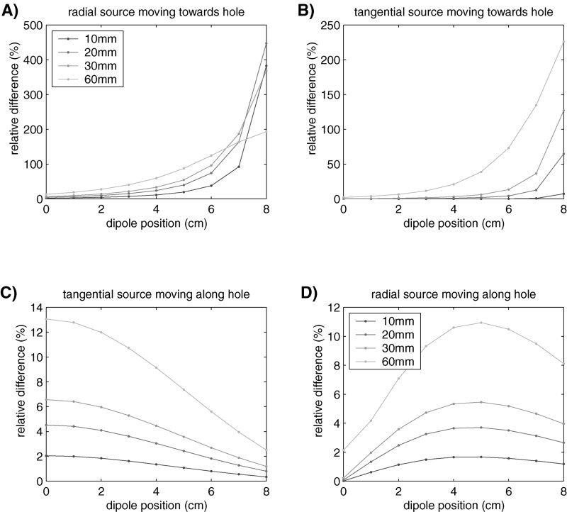
Potential difference between the BEM model without a hole and with hole of varying diameter, expressed as relative difference. The top row shows the difference for a source moving along the z‐axis from the center of the sphere toward the hole. The bottom row shows the difference for a hole moving orthogonal to (or along) the hole along the y‐axis. In the left column the source is oriented along the z‐axis (pointing in the direction of the hole), in the right column the source is oriented along the y‐axis (pointing orthogonal to the hole).
The effect of the hole on the potential distribution is shown in more detail in Figure 5, where the potential is plotted for a contour over the surface, running from directly above the hole at the positive z‐axis (θ = 0 degrees) toward the negative z‐axis (θ = 180 degrees), which also is the location of the reference electrode. Six figures are shown, each containing the potential for the model without a hole and for the models with a hole of 10, 20, 30, and 60 mm. The three columns represent different source locations along the z‐axis, running from the center toward the hole (z = 0 cm, 4 cm, 8 cm). The two rows represent the potential for a radial (toward the hole) and for a tangential dipole orientation. For the radial source pointing toward the hole, these figures demonstrate that the hole affects the scalp potential up to 90 degrees away from the hole, regardless of its size. The influence of the hole on the potential is greater for the larger holes, but is already apparent for the smallest hole. The distance between the dipole and the hole appears to be a more dominating factor than the hole diameter. The lower three panels of Figure 5 show that for a tangential dipole the effect of the hole on the potential is less pronounced. This is the case particularly if the dipole is far away from the hole, compared to the hole diameter (lower left and middle figure). For a dipole closer to the hole, the effect on the potential remains small only if the hole is also small in size (e.g., 10 mm). A relatively large hole (>10 mm) with a tangential dipole nearby shows again profound effects on the potential over a large part of the scalp.
Figure 5.
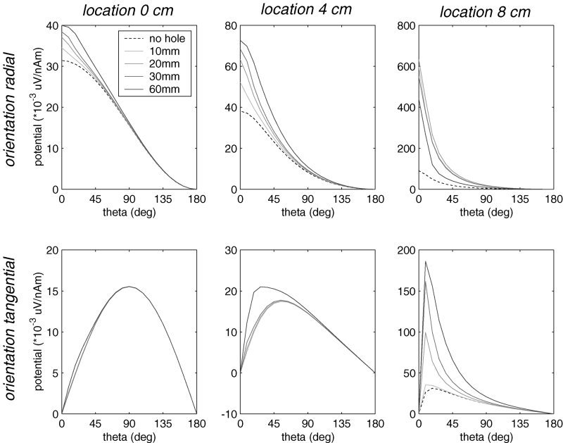
Potential difference between the BEM model without a hole and with a hole of varying diameter at θ = 180 degrees. The potential is plotted along a single contour over the surface; the reference for the potential is positioned at the side opposite the hole (θ = 180 degrees).
Influence of a hole on inverse dipole fitting
The influence of neglecting the presence of a hole in inverse computations is demonstrated in Figure 6. Forward potentials were computed using the BEM model with a hole of 20 mm on the z‐axis. The potential was computed at 642 evenly distributed electrodes with an average reference. A regular grid in the yz plane with a grid spacing of 1 cm was created and at each grid point a single dipole was placed. These dipoles were oriented either in the z‐direction, which is more or less in the direction of the hole, or in the y‐direction, which is more or less perpendicular to the hole. For each dipole location and orientation the forward potential was computed using the model with hole, and subsequently the dipole location was fitted using the model without the hole. The effect of neglecting the hole on the inverse calculations is displayed as the shift in dipole location: starting at each original (forward) grid location, an arrow is drawn toward the location where the (inverse) dipole was fitted. The length and direction of the arrow represents the shift in dipole location. It should be noted that the arrows have nothing to do with the dipole moment.
Figure 6.
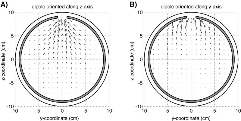
Influence of a 20‐mm hole on the location of a fitted dipole. The arrows indicate the error in dipole position, when an inverse model is used in which the hole is neglected. The dipole orientation is in the z‐direction for the left figure and in the y‐direction for the right figure. Note that the arrows do not indicate source orientation and strength.
Figure 6A shows the shift of the dipole oriented in the z‐direction, in Figure 6B the shift is shown for the y‐oriented dipoles. When oriented toward the hole, as for the largest part of Figure 6A, the fitted dipoles are shifted toward the hole. Figure 6B shows that dipoles oriented perpendicular to the hole tend to be pushed away from the hole, but still are located closer to the surface. Dipoles that are located near the hole display a shift of up to 1.5 cm. The shifts in location are small for dipoles located far away from the hole. We also carried out these forward and inverse computations for smaller and larger holes. As expected for a smaller (10‐mm) hole, the shifts in dipole location were slightly smaller than those displayed here for the 20‐mm hole, but with a same overall pattern in the error of the fitted dipole. With a hole of 30 mm, the shifts were accordingly larger.
DISCUSSION
We used analytical computed potentials for a one‐ and a three‐sphere volume conduction model for the head with no hole in the skull to evaluate the accuracy of the BEM and the FDM. The FDM proved to be very accurate, even for relatively coarse meshes. For a mesh of 200 × 100 nodes the RE of the FDM was <0.5% for a single sphere and less than 0.1% for a three‐sphere model. The accuracy of the BEM depends on the location of the source with respect to the interior brain and skull surfaces. The application of the isolated potential approach can greatly improve the accuracy of the BEM when using a regular mesh, from an error of 190% to an error of 10.8%. With a locally refined mesh near the source, the influence of the IPA is not so substantial, but its application still reduces the error from 10.4 to 3.5%. The IPA is not beneficial for deep sources. For superficial sources, a great increase in the accuracy of the BEM potential can also be achieved by using a locally refined mesh and the IPA is not necessary in that case. We conclude that beneficial effects of the IPA cannot clearly be indicated when holes are present in the skull. The use of a weighed IPA, as suggested by Fuchs et al. [1998], may provide a more optimal solution and deserves further investigation.
Using the FDM as a reference solution, we determined the accuracy of the BEM for a three‐sphere model with a hole in the skull. The comparison shows that both numerical methods give similar potentials. The differences between FDM and BEM range from 1.3 to 11.4%, but in most combinations of source location and hole size the difference is <5%. Due to the good performance of the FDM in the case of no hole, and due to the performance of the BEM when no hole is present (errors of 3.7–12.0%) we take the difference between the FDM and the BEM in the presence of a hole to reflect the inaccuracy of the BEM. We conclude that the BEM can be used to compute the potential with an error <12% for all configurations tested. Compared to the large effect the hole has on the potential (up to 450%), we consider this to be adequate.
The effect of holes in the skull on the scalp potential can be very large. Compared to a closed skull, potential differences of up to 200–450% are found when a dipole is present near the hole. The actual effect depends strongly on the location of the source with respect to the hole, but in general it is much larger for dipoles pointing toward the hole than for tangential dipoles. The results of inverse dipole fitting are strongly affected by the presence of a hole. Neglecting a hole in the skull leads to systematic errors in fitted source locations that can be up to several centimeters. In general, source locations are erroneously fitted closer to the hole for radial dipoles and closer to the surface for tangential dipoles. The effect of a hole on the forward and inverse computations using the BEM compares both quantitatively and qualitatively well to the FEM [van den Broek, 1997].
The comparison between FDM and BEM presented here demonstrates that the BEM can be used with confidence in the presence of holes in the skull.
REFERENCES
- Ary JP, Klein SA, Fender DH (1981): Location of sources of evoked scalp potentials: corrections for skull and scalp thickness. IEEE Trans Biomed Eng 28: 447–452. [DOI] [PubMed] [Google Scholar]
- Bank R, Sherman A, Weiser A (1983): Refinement algorithms and data structures for regular local mesh refinement In: Stepleman R, et al., editors. Scientific computing. Amsterdam: North Holland; p 3–17. [Google Scholar]
- Barnard CL, Duck IM, Lynn MS (1967a): The application of electromagnetic theory to electrocardiology. I. Derivation of the integral equations. Biophys J 7: 443–462. [DOI] [PMC free article] [PubMed] [Google Scholar]
- Barnard CL, Duck IM, Lynn MS, Timlake WP (1967b): The application of electromagnetic theory to electrocardiology. II. Numerical solution of the integral equations. Biophys J 7: 463–491. [DOI] [PMC free article] [PubMed] [Google Scholar]
- Berg P, Scherg M (1994): A fast method for forward computation of multiple‐shell spherical head models. Electroencephalogr Clin Neurophysiol 90: 58–64. [DOI] [PubMed] [Google Scholar]
- Buchner H, Waberski TD, Fuchs M, Wischmann HA, Wagner M, Drenckhahn R (1995): Comparison of realistically shaped boundary‐element and spherical head models in source localization of early somatosensory evoked potentials. Brain Topogr 8: 137–143. [DOI] [PubMed] [Google Scholar]
- Cuffin BN (1993): Effects of local variations in skull and scalp thickness on EEGs and MEGs. IEEE Trans Biomed Eng 40: 42–28. [DOI] [PubMed] [Google Scholar]
- Cuffin BN, Cohen D (1979): Comparison of the magnetoencephalogram and the electroencephalogram. IEEE Trans Biomed Eng 47: 131–146. [DOI] [PubMed] [Google Scholar]
- de Munck JC (1992): A linear discretization of the volume conductor boundary integral equation using analytically integrated elements. IEEE Trans Biomed Eng 39: 986–990. [DOI] [PubMed] [Google Scholar]
- Fuchs M, Dreckhahn R, Wischmann H, Wagner M (1998): An improved boundary element method for realistic volume‐conductor modeling. IEEE Trans Biomed Eng 45: 980–997. [DOI] [PubMed] [Google Scholar]
- Fuchs M, Wagner M, Kastner J (2001): Boundary element method volume conductor models for EEG source reconstruction. Clin Neurophysiol 112: 1400–1407. [DOI] [PubMed] [Google Scholar]
- Gabriel S, Lau RW, Gabriel C (1996): The dielectric properties of biological tissues. II. Measurements in the range of 10 Hz to 20 GHz. Phys Med Biol 41: 2251–2269. [DOI] [PubMed] [Google Scholar]
- Geddes LA, Baker LE (1967): The specific resistance of biological material, a compendium of data for the biomedical engineer and physiologist. Med Biol Eng Comput 5: 271–293. [DOI] [PubMed] [Google Scholar]
- Gilbert JR, Moler C, Schreiber R (1992): Sparse matrices in MATLAB: design and implementation. SIAM J Matrix Anal Appl 13: 333–356. [Google Scholar]
- Hämäläinen MS, Sarvas J (1989): Realistic conductivity geometry model of the human head for the interpretation of neuromagnetic data. IEEE Trans Biomed Eng 36: 165–171. [DOI] [PubMed] [Google Scholar]
- Huiskamp GJM, Vroeijenstijn M, van Dijk R, Wieneke G, van Huffelen AC (1999): The need for correct realistic geometry in the inverse EEG problem. IEEE Trans Biomed Eng 46: 1281–1287. [DOI] [PubMed] [Google Scholar]
- Kavanagh R, Darcey TM, Lehmann D, Fender DH (1978): Evaluation of methods for three‐dimensional localization of electric sources in the human brain. IEEE Trans Biomed Eng 25: 421–429. [DOI] [PubMed] [Google Scholar]
- Law SK (1993): Thickness and resistivity variations over the upper surface of he human skull. Brain Topogr 6: 99–109. [DOI] [PubMed] [Google Scholar]
- Leahy RM, Mosher JC, Spencer ME, Huang MX, Lewine JD (1998): A study of dipole localization accuracy for MEG and EEG using a human skull phantom. Electroencephalogr Clin Neurophysiol 107: 159–173. [DOI] [PubMed] [Google Scholar]
- Meijs JWH, Weier OA, Peters MJ, van Oosterom A (1989): On the numerical accuracy of the boundary element method. IEEE Trans Biomed Eng 36: 1038–1049. [DOI] [PubMed] [Google Scholar]
- Oostendorp TF, van Oosterom A (1989): Source parameter estimation in inhomogeneous volume conductors of arbitrary shape. IEEE Trans Biomed Eng 36: 382–391. [DOI] [PubMed] [Google Scholar]
- Oostendorp TF, Delbeke J, Stegeman DF (2000): The conductivity of the human skull: results of in vivo and in vitro measurements. IEEE Trans Biomed Eng 47: 1487–1492. [DOI] [PubMed] [Google Scholar]
- Pasqual‐Marqui RD, Michel CM, Lehmann D (1994): Low resolution electromagnetic tomography: a new method for localizing electrical activity in the brain. Int J Psychophysiol 18: 49–65. [DOI] [PubMed] [Google Scholar]
- Roth BJ, Ko D, von Albertini‐Carletti IR, Scaffidi D, Sato S (1997): Dipole localization in patients with epilepsy using the realistically shaped head model. Electroencephalogr Clin Neurophysiol 102: 159–166. [DOI] [PubMed] [Google Scholar]
- Scherg M, von Cramon D (1985): Two bilateral sources of the late AEPs as identified by a spatio‐temporal dipole model. Electroenceph Clin Neurophysiol 62: 32–44. [DOI] [PubMed] [Google Scholar]
- Scherg M, von Cramon D (1986): Evoked dipole source potentials of the human auditory cortex. Electroenceph Clin Neurophysiol 65: 344–360. [DOI] [PubMed] [Google Scholar]
- Sun M (1997): An efficient algorithm for computing multishell spherical volume conductor models in EEG dipole source localization. IEEE Trans Biomed Eng, 44: 1243–1252. [DOI] [PubMed] [Google Scholar]
- van Burik MJ (1999): Physical aspects of EEG. PhD thesis, University of Twente, The Netherlands.
- van den Broek S (1997): Volume conduction effects in EEG and MEG. PhD thesis. The Netherlands: University Twente. [DOI] [PubMed]
- van den Broek S, Reinders F, Donderwinkel M, Peters M (1998): Volume conduction effects in EEG and MEG. Electroenceph Clin Neurophysiol 106: 522–534. [DOI] [PubMed] [Google Scholar]
- Vanrumste B (2001): EEG dipole source analysis in a realistic head model. PhD thesis. Belgium: University Gent.
- Vanrumste B, van Hoey G, van de Walle R, D'Have M, Lemahieu I, Boon P (2000): Dipole location errors in electroencephalogram source analysis due to volume conductor model errors. Med Biol Eng Comput 38: 528–534. [DOI] [PubMed] [Google Scholar]
- Yvert B, Bertrand O, Echallier JF, Pernier J (1995): Improved forward EEG calculations using local mesh refinement of realistic head geometries. Electroencephalogr Clin Neurophysiol 95: 381–392. [DOI] [PubMed] [Google Scholar]
- Yvert B, Bertrand O, Echallier JF, Pernier J (1996): Improved dipole localization using local mesh refinement of realistic head geometries: an EEG simulation study. Electroencephalogr Clin Neurophysiol 99: 79–89. [DOI] [PubMed] [Google Scholar]