Model assessment and model building in fMRI

Abstract

Model quality is rarely assessed in fMRI data analyses and less often reported. This may have contributed to several shortcomings in the current fMRI data analyses, including: (1) Model mis‐specification, leading to incorrect inference about the activation‐maps, SPM{t} and SPM{F}; (2) Improper model selection based on the number of activated voxels, rather than on model quality; (3) Under‐utilization of systematic model building, resulting in the common but suboptimal practice of using only a single, pre‐specified, usually over‐simplified model; (4) Spatially homogenous modeling, neglecting the spatial heterogeneity of fMRI signal fluctuations; and (5) Lack of standards for formal model comparison, contributing to the high variability of fMRI results across studies and centers. To overcome these shortcomings, it is essential to assess and report the quality of the models used in the analysis. In this study, we applied images of the Durbin‐Watson statistic (DW‐map) and the coefficient of multiple determination (R ²‐map) as complementary tools to assess the validity as well as goodness of fit, i.e., quality, of models in fMRI data analysis. Higher quality models were built upon reduced models using classic model building. While inclusion of an appropriate variable in the model improved the quality of the model, inclusion of an inappropriate variable, i.e., model mis‐specification, adversely affected it. Higher quality models, however, occasionally decreased the number of activated voxels, whereas lower quality or inappropriate models occasionally increased the number of activated voxels, indicating that the conventional approach to fMRI data analysis may yield sub‐optimal or incorrect results. We propose that model quality maps become part of a broader package of maps for quality assessment in fMRI, facilitating validation, optimization, and standardization of fMRI result across studies and centers. Hum. Brain Mapping 20:227–238, 2003. © 2003 Wiley‐Liss, Inc.

INTRODUCTION

The appropriateness of the specific models employed in fMRI data analysis are currently justified by a priori knowledge about the hemodynamic response, as well as the end results of fMRI experiments, i.e., the activation‐maps. However, the quality of these models, i.e., how “good” these models are for the particular data in question, is rarely assessed and less often reported [Frsiton, 1998; Kherif et al., 2002; Petersson et al., 1999; Purdon et al., 2001; Razavi et al., 2001a–c; Strother et al., 2002]. The lack of model assessment may have contributed to several shortcomings in the current fMRI data analysis, including: (1) Model mis‐specification, resulting in incorrect inference about the activation‐maps, SPM{t} and SPM{F}; (2) Improper model selection based on the number of activated voxels, which has led to the incorrect view that the model producing the higher number of activated voxels, is the “better” model; (3) Under‐utilization of systematic model building (the process of specification, assessment, comparison, and selection of the “best” model), which has resulted in the common but suboptimal practice of using only a single, pre‐specified, usually over‐simplified model; (4) Spatially homogenous modeling, i.e., using the same pre‐specified model for each voxel, neglecting the spatial heterogeneity of fMRI signal fluctuations: and (5) Lack of standards for formal model comparison, contributing to the high variability of fMRI results across studies and centers. To overcome these shortcomings, i.e., to validate, optimize, and standardize fMRI results, it is essential to assess the quality of the models used in fMRI data analysis. The purpose of this study is to introduce the rationale for using and reporting images of classic diagnostic statistics, applicable to model assessment and model building in fMRI data analysis.

THEORY AND BACKGROUND

Model Assessment

To assess the appropriateness, i.e., quality, of a model, one needs to assess its validity as well as its goodness of fit [Kherif et al., 2002; Netter et al., 1996; Nichols and Luo, 2001; Petersson et al., 1999; Purdon et al., 2001; Razavi et al., 2001a–c].

Model validity

The extent to which the data in question satisfy the model assumptions determines the validity of the model and the subsequent statistical inference. General linear model (GLM), which is the most frequently used modeling approach in fMRI analysis [Friston et al, 1995a], has three assumptions, all of which relate to the error terms: (1) Normality, (2) Equal variance (homoscedasticity), and (3) Independence.

Neither normality nor homoscedasticity present serious problems for analysis of fMRI time series data [Nichols and Luo, 2001]. This is because for a large sample size such as fMRI time series data, the standard statistical tests are robust against violation of normality assumption [Pindyck and Rubinfeld, 1998]. Furthermore, homoscedasticity usually does not occur in time series data, because changes in the dependent and independent variables are of approximately the same magnitude [Pindyck et al., 1998]. In contrast, the independence assumption is often violated for time series data [Netter et al., 1996; Pindyck et al., 1998]. Therefore, in this study, we focus on the independence assumption.

Since the presence of “residual temporal autocorrelation” (RTAC) violates the independence assumption, its assessment can be used to evaluate the validity, and, therefore, the quality of the model employed in the analysis. Most fMRI data analysis methods acknowledge the existence of RTAC, and (usually without assessing it) adjust for it in two different ways: by shaping (“pre‐coloring”) or modeling (“pre‐whitening”) it [Bullmore et al., 1996, 2001; Friston et al. 1995a, b, 2000; Purdon et al., 2001; Petersson et al., 1999; Purdon and Weisskoff, 1998; Woolrich et al., 2001; Worsely and Friston, 1995; Zarahn et al., 1997]. However, both these adjustments have themselves assumptions about the amount of RTAC, which need to be tested [Bullmore et al., 1996, 2001; Purdon and Weisskoff, 1998; Purdon et al., 2001; Woolrich et al., 2001]. Since the magnitude of RTAC is setting‐dependent (experiment design, TR, pulse sequence, etc) [Burock and Dale, 2000; Purdon and Weisskoff, 1998], the adequacy of these adjustments needs to be evaluated for each individual fMRI study. Thus, in short, assessing RTAC after the adjustments is necessary to evaluate the validity of the adjustments, while assessing RTAC before the adjustment can be used as an indicator for the validity, and, therefore, the quality of the model(s) employed in the analysis.

To assess RTAC, previous studies applied images of square roots of autoregressive (AR) power of the residual terms [Bullmore et al., 2001; Worsley et al., 2002]. Since residual terms of fMRI time series are predominantly first‐order autocorrelated [Bullmore et al., 1996; Purdon and Weisskoff, 1998; Worsley et al., 2002], we used a widely applied statistic that tests for first‐order autocorrelation [AR(1)]: the Durbin‐Watson statistic (DW) [Nichols and Luo, 2001; Pindyck et al., 1998; Razavi et al., 2001a–c]:

(1)

Using the DW table [Netter et al., 1996], it can be determined whether statistical significance is reached. If there is no statistically significant DW, the independence assumption is not violated and the model is valid. However, if there is statistically significant DW, the model is not valid, and the subsequent inference for the model parameters such as regression coefficients, and consequently, the conventional activation‐maps, SPM{t} and SPM{F}, will be incorrect.

Model goodness of fit

The quality of a model does not only depend on its validity, but also on its closeness to the data in question, i.e., on its “goodness of fit”. A commonly used statistic for assessing model goodness of fit is the coefficient of multiple determination, R² [Netter et al., 1996; Vispoel, 1998]. R ² is the ratio of the magnitude of signal variance explained by the model to the magnitude of the total observed signal variance.

(2)

where SSR and SST are the regression (modeled) and the total sums of squares, respectively. The presence of RTAC will bias R ², emphasizing again the necessity to assess model validity before model goodness of fit. Once R ² is assessed, its statistical significance, i.e., whether the model explains a statistically significant amount of variance in the data, needs to be tested [Netter et al., 1996; Pindyck et al., 1998]:

(3)

where n is the number of observations and p the number of explanatory variables used in the model. Under the null hypothesis, this ratio follows an F distribution with (p ‐ 1, n ‐ p) degrees of freedom. Using the F table, it can then be determined whether statistical significance is reached. Note that F(R ²) is the same as the F‐statistic for the overall model. Thus, an SPM{F}(R ²) would be a map of the “overall” F statistic for all regression coefficients (pertaining to both effects of interest and no interest), which is different than the conventional omnibus SPM{F} that is a map of “partial” F statistic for a subset of regression coefficients (pertaining only to the effects of interest) [Friston et al., 1995], or the conventional SPM{t} that is a map of t statistic for a single regression coefficient (pertaining only to one effect of interest).

Relating the test of the overall model (R ²) to the tests of individual or a subset of regression coefficients is not trivial and has been the subject of debate [Bertrand and Holder, 1988; Cramer, 1972; Geary and Lese, 1968; Largey and Spencer, 1996]. What should the experimenter then do in the way of significance tests in regression? It has been established that the test of the overall model has precedence over the tests of individual or a subset of regression coefficients [Cramer, 1972; Geary and Lese, 1968]. Thus, one should first test the overall model. If the overall model (R ²) is not significant, then there is no reason to do further tests, because further interpretation of regression coefficients, even if they were significant, is incorrect. This situation may occur when too many irrelevant variables are included in the model. Here, remedies such as model simplification are, however, available. On the other hand, one should not discard an overall model that is significant, even if all regression coefficients are insignificant. This situation may occur, when there is multi‐collinearity between the independent variables [Andrade et al., 1999]. Here, remedies such as variable transformation are available. Thus, in short, failure to assess the goodness of fit of the overall model can lead to incorrect inference about the model parameters such as the regression coefficients, and consequently, the conventional activation‐maps, SPM{t} and SPM{F}.

Once the model goodness of fit proves to be statistically significant, its magnitude becomes a meaningful indicator for the quality of the model. While R ² is routinely used to assess the statistical significance of a model goodness of fit, as we described above, it has two shortcomings for being an indicator for the magnitude of goodness of fit. First, R ² is only comparable between models that are subsets of each other, and not between models that contain different explanatory variables. Secondly, R ² does not account for the number of variables used in the model. Indeed, adding more variables into the model can only increase R ², but never reduce it. However, any statistic to be used as an indicator for the magnitude of model goodness of fit should account for the number of variables used in the model, i.e., avoid over‐fitting, and allow comparison between models that contain different explanatory variables. While there are several such statistics, such as Akaike or Schwartz information criterion (AIC, BIC) [Ardekani et al., 1999; Pindyck et al., 1998], or NURE (nearly unbiased risk estimator) [Purdon et al., 2001], we used a classic, intuitive, and widely applied statistic that is closely related to R ²: the adjusted coefficient of multiple determination (R _a ²) [Netter et al. 1996; Razavi et al., 2001a–c]:

(4)

R _a ² is the proportion of the signal variance explained by the model, i.e., the ratio of the magnitude of signal variance explained by the model to the magnitude of the total observed signal variance, adjusted for the number of explanatory variables used in the model. The magnitude of R_a ² ranges between 0 being no fit, and 1 being the perfect fit, events that rarely occur in practice. Although R ² can only increase, R _a ² may also decrease, when more explanatory variables are added into the model. While penalizing for the number of variables used in the model, higher R_a ² indicates higher goodness of fit and, therefore, higher quality for the model. Thus, among models that are valid and have statistically significant goodness of fit, the model that has the higher magnitude of goodness of fit, i.e., higher R_a ², is the “better” model.

Model Comparison

Thus far we have discussed how to assess the quality of a model, in the correct order of its subcomponents: (1) validity; (2) statistical significance of goodness of fit; (3) magnitude of goodness of fit. Assessment of model quality is prerequisite for model comparison. Proper model comparison necessitates comparing models based on their quality, and not as done in the current fMRI time series analyses, based on the number of activated voxels, i.e., statistical significance of individual or subset of regression coefficients. Thus, while in the current fMRI time series analysis, the model that leads to the highest number of activated voxels is selected, proper modeling necessitates selecting the model with the highest quality, i.e., a model that is valid and has the statistically significant and highest goodness of fit, even if the number of activated voxels is lower; and discard the model that is not valid or has a statistically insignificant or lowest goodness of fit, even if the number of activated voxels is higher.

Model Building

Model assessment and model comparison are necessary prerequisites for model building, which is a process of using statistical as well as substantive (such as biological plausibility) evidence for selecting a set of explanatory variables, to achieve a model with the highest quality, i.e., the “best” model [Netter et al., 1996]. There are several model‐building procedures such as “all possible regression,” “forward selection,” “backward elimination,” and “stepwise selection.” Although “all possible regression” is the most frequently used procedure among statisticians, it is usually not applied for explanatory data analysis. In this study, we used the “forward selection” procedure. One usually starts with the simplest model (reduced model) and builds it up with subsequent addition of explanatory variables, one at a time, as long as the addition, while verifying the validity and the statistical significance of the goodness of fit of the new model (the full model) improves the magnitude of the goodness of fit of the reduced model. Although this improvement can be assessed using the magnitude of R _a ², because here the reduced model is a subset of the full model, one can also employ the magnitude of R ², the improvement of which can be further assessed for statistical significance:

(5)

In contrast to R _a ², which itself adjusts for the number of variables used in the model, in the case of R ², the degrees of freedom for the F test make the adjustment in a different way. If the increment is statistically significant, then the full model is “improved” and will be “selected.” This full model serves, in turn, as a reduced model for further model building, i.e., subsequent addition of a new explanatory variable, and the process starts anew. One stops when addition of the new variable does not lead to a statistically significant increment, i.e., when the new variable is inappropriate. The final “best” model is a model that is valid and has the statistically significant and highest goodness of fit.

In summary, we have described why and how to assess, compare, and build models. Next we will apply these approaches to fMRI time series data.

SUBJECTS AND METHODS

Six healthy subjects were studied. Informed consent was obtained. BOLD‐contrast, gradient echo‐planar fMRI images were acquired on a 1.5T GE scanner: TE 40 msec, TR and flip angle: 1 sec and 60 degrees, or 3 sec and 90 degrees, FOV 24 cm, acquisition matrix 64 × 64 or 128 × 128, slice thickness 5 mm, number of slices 5, number of time points 102, total number of scans 510. The I/OWA “time aware” data acquisition system was used [Smyser et al., 2001]. Subjects viewed a rotating right hemifield 8‐Hz inverting checkerboard with a period of 20 sec.

Data Analysis

All functional EPI‐BOLD images were motion‐corrected, using AIR 3.03 [Woods et al., 1992]. Analysis was performed voxelwise with tal_regress that implements GLM [Frank et al., 1997]. The task variable was obtained by convolving the stimulus time function with a pre‐defined hemodynamic response function [Cohen, 1997]. Physiologic variables were the amplitude of chest expansion and the timing of the cardiac cycle. Variables representing low‐frequency (<0.1 Hz) fMRI signal fluctuations were a linear trend or sine and cosine functions with 0.001, 0.003, 0.01 Hz frequency.

Activation maps were computed by generating a t‐ map of the estimated regression coefficient for the task variable and thresholding at P = 0.01 for statistical significance.

Model validity was assessed by computing, the mean DW over all voxels, images of DW (DW‐maps), and DW‐maps thresholded with corresponding values from the DW table at P = 0.01 (significance‐ thresholded DW‐maps). Model goodness of fit was assessed by computing, the mean R ² and R _a ² over all voxels, images of R ² and R _a ² ( R ²‐ and R _a ²‐maps), and R ²‐maps thresholded with corresponding values from the F table at P = 0.01 (significance‐thresholded F(R ²)‐maps).

Model building was performed using forward selection procedure, as described in the theory section. To assess the effect of adding a variable on model validity, we computed the difference between the significance‐thresholded DW‐maps of the reduced and the full model, which displayed voxels where DW became insignificant, i.e., where the model became valid, once the variable was added to the reduced model (hereafter called the “model validity‐improvement‐map” or DW improvement‐map”). To assess the effect of adding a variable on model goodness of fit, we computed the significance‐thresholded F(R ²)‐maps for the reduced and the full model, which displayed voxels where the goodness of fit of each model was significant, and then the “R ²increment‐map”, which displayed voxels where the goodness of fit improved significantly, once the variable was added to the reduced model (hereafter called the “model goodness of fit improvement‐map or ”R ² improvement‐map“). The opposite effects, i.e., lower validity and goodness of fit were insignificant, except when indicated (e.g., model mis‐specification). Once the validity, the goodness of fit, and the increment proved to be statistically significant, then the full model was “improved” and “selected.” This full model served, in turn, as the reduced model for all subsequent model building.

Model quality maps were computed with and without including variables representing task, cardiac, respiratory, and low frequency effects. The effect of sample size on model quality was assessed by combining data from two runs (i.e., doubling the sample size) and comparing it to the average of these maps over the individual runs. The effects of spatial smoothing (FWHM = 2 voxels), acquisition matrix size (64 × 64, 128 × 128), and sampling rate (TR 1 vs. 3 sec) on model quality were also assessed.

RESULTS

Figure 1 demonstrates how model quality maps track the improvement in model quality, after adding the task variable to the reduced model. Thus, the “reduced” model consisted of constant term + global mean signal intensity, while the “full” model consisted of reduced model + task variable. First, the significance‐thresholded DW and F(R ²)‐maps for the reduced model are shown (Fig. 1C,D). There is significant DW and insignificant R ² in several areas including voxels in the occipital lobe, suggesting unmodeled effects in those areas. Adding the task variable to the reduced model resulted in different significance‐thresholded DW and F(R ²)‐maps for the full model (Fig. 1E,F). A comparison of DW‐ and R ²‐improvement‐maps (Fig. 1G,H) demonstrates, as expected, that adding the task variable to the reduced model, improved validity and goodness of fit in spatially similar voxels in the occipital lobe. Thus, the full model including the task variable was “improved” and “selected.” This full model served, in turn, as the reduced model for all subsequent model building.

Figure 1.

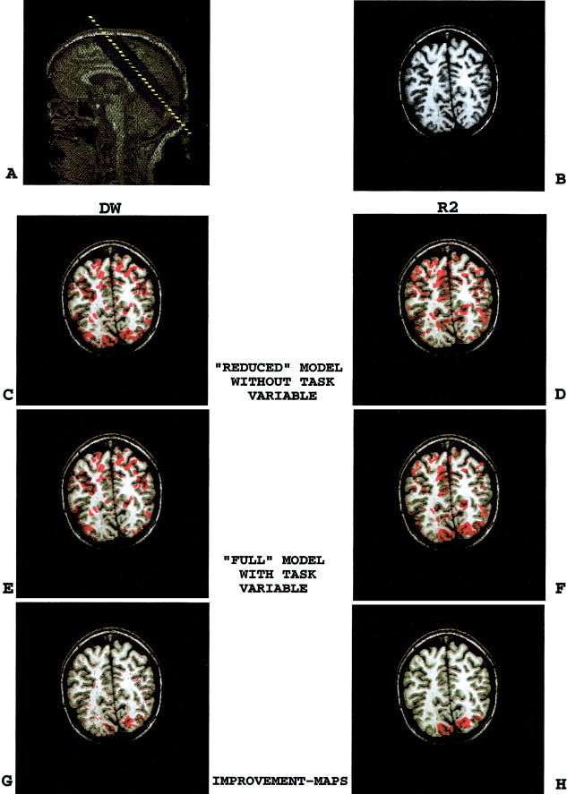
(overleaf). Model quality maps track the task effect. To demonstrate the appropriateness of model quality maps for model assessment and model building, we used an exercise of intentionally failing to model a known task effect in a benchmark visual stimulation paradigm. A comparison of DW‐ and R ²‐improvement‐maps (GH) demonstrates, as expected, that adding the task variable to the reduced model, improved validity and goodness of fit of the reduced model in spatially similar voxels in the occipital lobe. Thus, the full model including the task variable was “improved” and “selected.” This full model served, in turn, as the reduced model for all subsequent model building. A,B: Anatomical images. A: Sagittal scout image and slice orientation. B: SPGR T₁‐weighted anatomical image. C,D: Reduced model (model without the task variable). C: Significance‐thresholded DW‐map. D: Significance‐thresholded F(R ²)‐map. E,F: Full model (model with the task variable). E: Significance‐thresholded DW‐map. F: Significance‐thresholded F(R ²)‐map. G,H: Model quality improvement‐maps. G: DW‐improvement‐map. Red voxels indicate where DW for the overall model becomes insignificant, i.e., model becomes valid, once the task variable is added to the reduced model (C–E). H: R ²‐improvement‐map. Red voxels indicate where R ² of the reduced model improved significantly, once the task variable is added to the reduced model (F–D).

Figure 2 shows DW and R ² improvement‐maps after adding variables representing cardiac, respiratory, and low frequency periodic effects for the combined frequencies of 0.01, 0.003, and 0.001. The improvement in model validity and goodness of fit were again in spatially similar voxels. The improvements provided by adding the cardiac, respiratory, and low‐frequency variables to the model were located near large blood vessels (Fig. 2B,C), widespread (Fig. 2D,E), and in the cortical gray matter (Fig. 2F,G), respectively. The improvement provided by adding low‐frequency variables to the model were more prominent than those by adding cardio‐respiratory variables.

Figure 2.

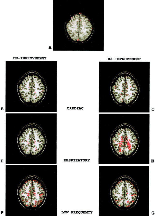
(p 233). Model quality improvement‐maps after adding physiologic variables to the model. A comparison of left to right panel demonstrates that adding physiologic variables such as cardiac, respiratory, and low‐frequency periodic functions to the reduced model improved both the validity and the goodness of fit of the reduced model in spatially similar voxels. Note that the low‐frequency periodic effects were more prominent than cardio‐respiratory effects. A: Map of blood vessels. B,C: DW‐ and R ²‐improvement‐maps for the cardiac variable. D,E: DW‐ and R ²‐improvement‐maps for the respiratory variable. F,G: DW‐ and R ²‐improvement‐maps for the low‐frequency periodic variable.

Next we compared two different approaches currently used to model low‐frequency fluctuations of fMRI signal: linear trend vs. periodic functions. These two approaches behaved differently with respect to the DW statistic. While periodic functions decreased the significance of DW, i.e., improved model validity, linear detrending increased DW, i.e., diminished model validity (Fig. 3A,C). Both variables, however, improved R ² in spatially similar regions (Fig. 3B,D).

Figure 3.

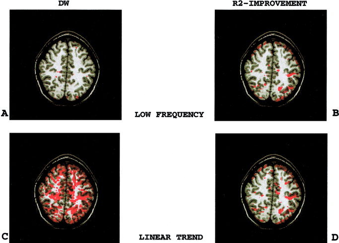
Comparison of low‐frequency periodic functions to linear detrending. Both linear trend and low‐frequency periodic functions improved the model goodness of fit. However, fewer voxels had significant DW values, i.e., invalid model, when the model included low‐frequency periodic functions as compared to a linear trend. A: Significance‐thresholded DW‐map for the model including low‐frequency periodic functions. B: R ²‐improvement‐map for the low‐frequency periodic functions. C: Significance‐thresholded DW‐map for the model including a linear trend. D: R ²‐improvement‐map for the linear trend.

The spatial results of model quality maps can be summarized by averaging them over the entire brain. Table I provides the results of model building for a single subject. Non‐thresholded R _a ²‐map summaries are provided as well. Using a forward selection procedure, we started with the simplest (reduced) model (constant term + global mean signal intensity), and built it up with the subsequent addition of different explanatory variables, e.g., task, cardiac, respiratory, low‐frequency periodic functions, and linear trend. Indeed, all explanatory variables improved model quality, and were, therefore, appropriate to be included in the final full model, except for the linear trend. Note that while linear detrending diminished model validity, it improved model goodness of fit as well as the number of activated voxels. On the other hand, although adding the cardiac variable to the model improved both model goodness of fit and validity, it decreased the number of activated voxels. Table II summarizes the averaged results for all subjects.

Table I.

Model assessment and model building for one subject*

Models	DW Mean	DW‐map (% volume improved)	R ${}_{\mathit{\text{a}}}^{\text{2}}$ Mean	R ${}_{\mathit{\text{a}}}^{\text{2}}$ Max	R 2‐map (% volume improved)	No. of activated voxels
Constant term and global	1.61	—	0.15	0.74	—	—
+ Task	1.63	2	0.16	0.76	8	310
+ Cardiac	1.63	2	0.19	0.81	8	−14
+ Resp	1.63	1	0.18	0.80	15	+2
+ Low Frequency	1.93	23	0.30	0.95	16	+85
+ Linear trend	1.20	−32	0.27	0.90	22	+37

^*Model validity was assessed with DW. Model goodness of fit was assessed with R ² and R _a ². While DW and R _a ² means were not thresholded, the DW‐ and R ² improvement‐maps were thresholded at P = 0.01 and, therefore, statistically significant. The proportion of voxels with statistically insignificant DW and significant R ² was used as an indicator for model quality. The “reduced” model consisted of constant term + global mean signal intensity. Adding the task variable to the reduced model improved model goodness of fit and validity. This improved “full” model including the task variable, served, in turn, as the reduced model for all subsequent model building.

Table II.

Model assessment and model building averaged for six subjects*

Models	DW‐map (% volume improved)	R 2‐map (% volume improved)
+ Task	4 ± 1	6 ± 4
+ Cardiac	2 ± 4	4 ± 7
+ Resp	2 ± 2	5 ± 6
+ Low frequency	17 ± 9	17 ± 13
+ Linear trend	−22 ± 7	14 ± 12

^*See legend for Table I.

Table III demonstrates the changes in model quality resulting from spatial smoothing, coarser acquisition matrix, increasing sample size, or shortening TR. Spatial smoothing as well as coarser acquisition matrix improved model goodness of fit but diminished model validity. Increasing sample size as well as shortening TR improved both model validity as well as model goodness of fit.

Table III.

Effect of acquisition parameters and data transformation on model quality maps averaged for six subjects*

Models	DW‐map (% volume improved)	R 2‐map (% volume improved)
+ Task	4 ± 1	6 ± 4
Smooth (2 × 2)	−10 ± 5	20 ± 15
4× increase in Voxel size	−20 ± 19	30 ± 25
2× increase in time points	2 ± 6	36 ± 26
TR 1	19 ± 1	17 ± 6

^*See legend for Table I.

DISCUSSION

We applied images of model validity (DW‐maps) and model goodness of fit (R ²‐ map) as complementary tools to assess and build models in fMRI time series analysis.

The appropriateness of these model quality maps was demonstrated through the exercise of intentionally failing to model a known task effect in a benchmark visual stimulation paradigm. Under these circumstances, one would expect that the model quality maps would identify an unmodeled effect (invalid model and insignificant goodness of fit) in the occipital lobe. This was indeed the case. Moreover, as expected, adding the task effect to the model improved the validity (DW‐improvement‐map) and the goodness of fit (R ²‐improvement‐map) of the overall model in spatially similar voxels in the occipital lobe. Although DW‐ and R ²‐improvement‐maps both indicate modeled effects, they are not identical. While R ²‐improvement‐maps indicate modeled effects of all lag‐terms, DW‐improvement‐maps indicate modeled effects of only first‐order lag‐terms. Partitioning RTAC into higher‐order lag‐terms [Cryer 1994; Locascio et al., 1997; Tagaris et al., 1997], and computing their corresponding maps, may point out to the different processes (e.g., seasonal effects) contributing to unmodeled effects, i.e., noise.

To further demonstrate the utility of these model quality maps in model building, several examples of modeling physiologic noise were demonstrated. Using receiver operating characteristic curve (ROC) analysis, previous reports showed that including physiologic and first‐order autocorrelated [AR (1)] effects into the model reduced false‐positive activation [Biswal et al., 1996; Buonocore and Maddock, 1997; Dagli et al., 1999; Hu et al., 1995; Le and Hu, 1996, 1997; Purdon and Weisskoff, 1998]. These findings support the conventional view that RTAC in fMRI time series is due to unmodeled physiologic effects, but this has not been explicitly demonstrated yet. If RTAC were due to unmodeled physiologic fluctuations as previously suggested, statistically significant RTAC should be present around regions reported to be affected by physiologic fluctuations, and modeling the physiologic fluctuations should improve RTAC and R ² in spatially similar voxels in those regions. This was indeed demonstrated. The improvement in model quality, however, was not necessarily associated with an improvement in the number of activated voxels. For example, including the cardiac variable improved the quality of the model, but decreased the number of activated voxels. Thus, while model assessment indicated that it was more appropriate to include the cardiac variable in the model, had we used the conventional approach to fMRI analyses, the model with the higher quality, i.e., the “better” model, would have been discarded.

In the previous examples of model building, we have demonstrated that inclusion of an appropriate variable in the model improved model quality. However, inclusion of an inappropriate variable in the model, i.e., model mis‐specification, may adversely affect model quality. Below we discuss one example of such model mis‐specification [Pindyck et al., 1998], where a commonly used preprocessing technique, linear detrending, while improving the model goodness of fit, adversely affects model validity.

Low‐frequency fluctuations in fMRI signal are commonly modeled with either linear detrending or discrete cosine basis functions [Bandettini et al., 1993; Holmes et al., 1997]. The choice is arbitrary, and no formal comparison of these two approaches has been made. Using model quality maps, we demonstrated that both variables improved the number of activated voxels as well as the goodness of fit of the model. However, only the periodic functions improved the validity of the model, whereas linear trend diminished it. Thus, while the conventional analysis and indeed the current practice allow using any of the two variables arbitrarily, model quality assessment clearly demonstrated the superiority of periodic functions to linear trend. This finding is consistent with previous suggestions that the fMRI signal drift is not linear but sinusoidal with a period of several minutes [Marchini and Ripley, 2000; Skudlarski et al., 1999].

The second example where improvement in model goodness of fit was associated with diminished model validity involved two maneuvers that increase the signal‐to‐noise ratio: spatial smoothing and larger voxel size. These maneuvers reduced the proportion of random noise in the unmodeled variance, so that the remaining systematic unmodeled variance, i.e., RTAC, became more prominent relative to random noise, resulting in an increase in the significance of RTAC. These maneuvers would not lead to decreased model validity if the processes giving rise to RTAC were modeled.

The amount of RTAC depended on TR and acquisition matrix size, possibly due to RTAC dependency on the signal‐to‐noise ratio [Purdon and Weisskoff, 1998; Turner et al., 1998; Zarahn et al., 1997]. The sensitivity of model quality to acquisition parameters underscores the need to assess and report model quality routinely.

Currently, modeling techniques for fMRI time series apply the same explanatory model to every voxel. This approach runs the risk of under‐fitting for some voxels and over‐fitting for others. The spatial heterogeneity of DW and R ² indicates that data in some voxels are modeled better than data in others. Thus, an additional benefit of having model quality maps would be to provide an objective basis for adopting different models for different voxels. Such a spatially heterogeneous modeling approach has not been explored, but may prove beneficial, particularly for studying clinical populations with altered physiologic states (e.g., altered cerebral autoregulation) or anatomy (e.g., lesion).

Current fMRI literature often offers discrepant results produced by the same experiment. This has motivated the neuroimaging community to propose a shared database for formal comparison of results across different centers [Editorial, 2000; Roland et al., 2001]. Variability in results can originate from a variety of sources including the research subjects involved, the experimental setting (design, acquisition), or the data analysis, particularly the models employed. While the subject factor is dealt with through randomization, and the experimental setting and the analysis streams including the employed models are being standardized, the quality of these models for the particular data in question is rarely assessed or reported. If two identical experiments or even the same data are modeled differently, e.g., in terms of validity or goodness of fit (one 30% vs. the other 90%), one could expect to obtain different results. Thus, in order to compare fMRI results, it is essential to assess the quality of models used in the analyses.

We propose that the model quality maps, namely, images of model validity (DW‐maps) and model goodness of fit (R ²‐map), become part of a broader package of maps for quality assessment in fMRI. Such a package may include quality‐maps for: (1) other aspects of model and statistical analysis as a whole, e.g., model prediction‐map [Strother et al., 2002], non‐linearity map, interaction and confoundmaps, multi‐collinearity‐map (variance inflation factor‐map), outliers‐map (Cook's statistic map) [Cox, 2002; Nichols and Luo, 2002]; (2) post‐acquisition, pre‐modeling, image processing, e.g., the amount of motion correction applied (motion‐correction map) [Nichols and Luo, 2002]; and (3) acquisition, e.g., the extent of the scanned volume and the location of susceptibility artifacts (sensitivity‐map) [Parrish et al., 2000] and measurement error (reliability‐map) [Genovese et al., 1997; Maitra et al., 2002]. Issues related to experimental design, e.g., order, maturation, or history effect [Goodwin, 1998; Leary, 2001], resting condition [Raichle et al., 2001], baseline tasks [Newman et al., 2001; Stark and Squire, 2001], sample size [Friston et al., 1999], efficiency [Dale, 1999]; and subject factors, e.g., blood pressure, hematocrit [Levin et al., 2001], anxiety, and intake of lipid [Noseworthy et al., 2003], alcohol, nicotine, or caffeine [Cohen et al., 2002], which cannot be assessed with maps, need to be considered as well. Since all these factors contribute to the variability of fMRI results, their quantitative assessment and routine reporting, and their experimental or statistical control, are essential to facilitate comparison and appraisal of fMRI results across studies and centers.

Like any other scientific research, fMRI research starts with developing a theory, deducing a hypothesis from the theory, and testing the hypothesis with an experiment [Goodwin, 1998; Kirk, 1995; Leary, 2001; Thorndike, 1997]. The latter involves: designing the experiment (paradigm, setting, subjects), conducting the experiment through measurement of dependent and independent variables, and analysis of the experimental (measured) data (post‐processing, modeling, and inference). The term “validity” extends to all these different levels of the research project, including: deducing the hypothesis from the theory (construct validity), the experimental design (internal and external validity), measurement (measurement validity, for which, reliability is a pre‐condition), and finally the data analysis (statistical conclusion validity). While in this study we addressed model validity, assessing and reporting the validity of each step would be necessary to ensure the validity of the research study as a whole.

REFERENCES

- Andrade A, Paradis A‐L, Rouquette S, Poline J‐B (1999): Ambiguous results in functional neuroimaging data analysis due to covariate correlation. NeuroImage 10: 483–486. [DOI] [PubMed] [Google Scholar]
- Ardekani BA, Kershaw J, Kashikura K, Kanno I (1999): Activation detection in functional MRI using subspace modeling and maximum likelihood estimation. IEEE Transactions on Medical Imaging 18: 101–114. [DOI] [PubMed] [Google Scholar]
- Bandettini PA, Jesmanowicz A, Wong EC, Hyde JS (1993): Processing strategies for time‐course data sets in functional MRI of the human brain. Magn Reson Med 30: 161–173. [DOI] [PubMed] [Google Scholar]
- Bertrand P, Holder RL (1988): A quirk in multiple regression: the whole regression can be greater than the sum of its parts. Statistician 37: 371–374. [Google Scholar]
- Biswal B, DeYoe EA, Hyde JS (1996): Reduction of physiological fluctuations in fMRI using digital filters. Magn Reson Med 35: 107–113. [DOI] [PubMed] [Google Scholar]
- Bullmore E, Brammer M, Williams SCR, Rabe‐Hesketh S, Janot N, David A, Mellers J, Howard R, Sham P (1996): Statistical methods of estimation and inference for functional MR image analysis. Magn Reson Med 35: 261–277. [DOI] [PubMed] [Google Scholar]
- Bullmore E, Long C, Suckling J, Fadili J, Calvert G, Zelaya F, Carpenter TA, Brammer M (2001): Colored noise and computational inference in neurophysiological (fMRI) time series analysis: Resampling methods in time and wavelet domains. Hum Brain Mapp 12: 61–78. [DOI] [PMC free article] [PubMed] [Google Scholar]
- Buonocore MH, Maddock RJ (1997): Noise suppression digital filter for functional magnetic resonance imaging based on image reference data. Magn Reson Med 38: 456–469. [DOI] [PubMed] [Google Scholar]
- Burock MA, Dale AM (2000): Estimation and detection of event‐related fMRI signals with temporally correlated noise: a statistically efficient and unbiased approach. Hum Brain Mapp 11: 249–260. [DOI] [PMC free article] [PubMed] [Google Scholar]
- Cohen ER, Ugurbil K, Kim S‐G (2002): Effect of basal conditions on the magnitude and dynamics of the blood oxygenation level‐dependent fMRI response. J Cereb Blood Flow Metab 22: 1042–1053. [DOI] [PubMed] [Google Scholar]
- Cohen MS (1997): Parametric analysis of fMRI data using linear systems methods. NeuroImage 6: 93–103. [DOI] [PubMed] [Google Scholar]
- Cox RW (2002): Outlier detection in fMRI time series. Proc Intl Soc Mag Reson Med 10. [Google Scholar]
- Cramer EM (1972): Significance tests and tests of models in multiple regression. Am Stat 26: 26–30. [Google Scholar]
- Cryer JD (1994): Time series analysis. Boston: Duxbury Press; p 25–52 [Google Scholar]
- Dagli MS, Ingeholm JE, Haxby JV (1999): Localization of cardiac‐induced signal change in fMRI. Neuroimage 9: 407–415. [DOI] [PubMed] [Google Scholar]
- Dale AM (1999): Optimal experimental design for event‐related fMRI. Hum Brain Mapp 8: 109–114. [DOI] [PMC free article] [PubMed] [Google Scholar]
- Editorial (2000): A debate over fMRI data sharing. Nature Neurosci 3: 845–846. [DOI] [PubMed] [Google Scholar]
- Frank RJ, Damasio H, Grabowski TJ (1997): Brainvox: an interactive, multimodal visualization and analysis system for neuroanatomical imaging. Neuroimage 5: 13–0. [DOI] [PubMed] [Google Scholar]
- Friston KJ (1998): Imaging neuroscience: principles or maps? Proc Natl Acad Sci USA 95: 796–802. [DOI] [PMC free article] [PubMed] [Google Scholar]
- Friston KJ, Holmes AP, Worsley KJ, Poline J‐P, Frith CD, Frackowiak RSJ (1995a): Statistical parametric maps in functional imaging: a general linear approach. Hum Brain Mapp 2: 189–210. [Google Scholar]
- Friston KJ, Holmes AP, Poline J‐B, Grasby PJ, Williams SCR, Frackowiak RSJ, Turner R (1995b): Analysis of fMRI time‐series revisited. Neuroimage 2: 45–53. [DOI] [PubMed] [Google Scholar]
- Friston KJ, Holmes AP, Worsley KJ (1999): How many subjects constitute a study? Neuroimage 10: 1–5. [DOI] [PubMed] [Google Scholar]
- Friston KJ, Josephs O, Zarahn E, Holmes AP, Rouquette S, Poline J‐B (2000): To smooth or not to smooth? Bias and efficiency in fMRI time‐series analysis. Neuroimage 12: 196–208. [DOI] [PubMed] [Google Scholar]
- Geary RC, Lese CEV (1968): Significance tests in multiple regression. Am Stat 22: 20–21. [Google Scholar]
- Genovese CR, Noll DC, Eddy WF (1997): Estimating test‐retest reliability in functional MR imaging. I: statistic methodology. Magn Reson Med 38: 497‐507. [DOI] [PubMed] [Google Scholar]
- Goodwin CJ (1998): Research in psychology. New York: John Wiley and Sons; p 99–169. [Google Scholar]
- Holmes AP, Josephs O, Büchel C, Friston KJ (1997): Statistical modeling of low‐frequency confounds in fMRI. Neuroimage 5: S480. [Google Scholar]
- Hu X, Le TH, Parrish T, Erhard P (1995): Retrospective estimation and correction of physiological fluctuation in functional MRI. Magn Reson Med 34: 201–212. [DOI] [PubMed] [Google Scholar]
- Kirk RE. (1995): Experimental design, 3rd ed. Pacific Grove, CA: Brooks and Cole; p 16–24. [Google Scholar]
- Kherif F, Poline J‐B, Flandin, G , Benali H, Simon O, Dehaene S, Worsley KJ (2002): Multivariate model specification for fMRI data. Neuroimage 16: 1068–1083. [DOI] [PubMed] [Google Scholar]
- Largey A, Spencer JE (1996): F‐and t‐tests in multiple regression: the possibility of ‘conflicting’ outcomes. Statistician 45: 105–109. [Google Scholar]
- Le TH, Hu X (1996): Retrospective estimation and correction of physiological artifacts in fMRI by direct extraction of physiological activity from fMRI data. Magn Reson Med 35: 290–298. [DOI] [PubMed] [Google Scholar]
- Le TH, Hu X (1997): Methods for assessing accuracy and reliability in functional MRI. NMR Biomed 10: 160–164. [DOI] [PubMed] [Google Scholar]
- Leary MR (2001): Introduction to behavioral research methods, 3rd ed. Boston: Allyn and Bacon; p 1–77. [Google Scholar]
- Levin JM, Frederick Bd, Ross MH, Fox JF, von Rosenberg HL, Kaufman MJ, Lange N, Mendelson JH, Cohen BM, Renshaw PF (2001): Influence of baseline hematocrit and hemodilution on BOLD fMRI activation. Magn Reson Imag 19: 1055–1062. [DOI] [PubMed] [Google Scholar]
- Locascio JJ, Jennings PJ, Moore CI, Corkin S (1997): Time series analysis in the time domain and resampling methods for studies of functional magnetic resonance brain imaging. Hum Brain Mapp 5: 168–193. [DOI] [PubMed] [Google Scholar]
- Maitra R, Roys SR, Gullapalli RP (2002): Test‐retest reliability estimation of functional MRI data. Magn Reson Med 48: 62–70. [DOI] [PubMed] [Google Scholar]
- Marchini JL, Ripley BD (2000): A new statistical approach to detecting significant activation in functional MRI. Neuroimage 12: 366–380. [DOI] [PubMed] [Google Scholar]
- Netter J, Kutner MH, Nachtsheim CJ, Wassermann W (1996): Applied linear statistical models, 4th ed. Chicago: Irwin; p 110–111, 230–231, 339–351, 504–507. [Google Scholar]
- Newman SD, Twieg DB, Carpenter PA (2001): Baseline conditions and subtractive logic in neuroimaging. Hum Brain Mapp 14: 228–235. [DOI] [PMC free article] [PubMed] [Google Scholar]
- Nichols TE, Luo WL (2001): Data exploration through model diagnosis. Neuroimage 13: S208. [Google Scholar]
- Nichols TE, Luo WL (2002): Diagnosis of linear models for fMRI. Proc Intl Soc Mag Reson Med 10: 753. [Google Scholar]
- Noseworthy MD, Alfonsi J, Bells S (2003): Attenuation of brain BOLD response following lipid ingestion. Hum Brain Mapp 20: 116–121. [DOI] [PMC free article] [PubMed] [Google Scholar]
- Parrish TB, Gitelman DR, LaBar KS, Mesulam MM (2000): Impact of signal‐to‐noise ratio on functional MRI. Magn Reson Med 44: 925–932. [DOI] [PubMed] [Google Scholar]
- Petersson KM, Nichols TE, Poline J‐B, Holmes AP (1999): Statistical limitations in functional neuroimaging 1. Non‐inferential methods and statistical models. Phil Trans R Soc Lond B 354: 1239–1260. [DOI] [PMC free article] [PubMed] [Google Scholar]
- Pindyck RS, Rubinfeld DL (1998): Econometric models and economic forecasts, 4th ed. Boston: Irwin/McGraw‐Hill; p 88–92, 112–113, 145–177, 164–166, 238–239, 317–318, 554–555. [Google Scholar]
- Purdon PL, Weisskoff RM (1998): Effect of temporal autocorrelation due to physiological noise and stimulus paradigm on voxel‐level false‐positive rates in fMRI. Hum Brain Mapp 6: 239–249. [DOI] [PMC free article] [PubMed] [Google Scholar]
- Purdon PL, Solo V, Weisskoff RM, Brown EN (2001): Locally regularized spatio‐temporal modeling and model comparison for functional fMRI. Neuroimage 14: 912–923. [DOI] [PubMed] [Google Scholar]
- Raichle ME, MacLeod AM, Snyder AZ, Powers WJ, Gusnard DA, Shulman GL (2001): A default mode of brain function. Proc Natl Acad Sci 98: 676–682. [DOI] [PMC free article] [PubMed] [Google Scholar]
- Razavi M, Grabowski TJ, Mehta S, and Bolinger L (2001a): Can improved statistical modeling reduce residuals temporal autocorrelation? International Society for Magnetic Resonance in Medicine (ISMRM) Annual Meeting, Scotland. Proc Intl Soc Mag Reson Med 2001; 9: 1747. [Google Scholar]
- Razavi M, Grabowski TJ, Mehta S, Bolinger L (2001b): The source of residual temporal autocorrelation in fMRI time series. Neuroimage 13: S228. [Google Scholar]
- Razavi M, Grabowski TJ, Mehta S, Allen, JS , Bolinger L (2001c): Model quality metrics for assessing linear models in fMRI time series analysis. Soc Neurosci Abstr 27: 83:12. [Google Scholar]
- Roland P, Svensson G, Lindeberg T, Risch T, Baumann P, Dehmel A, Frederiksson J, Halldorson H, Forsberg L, Young J, Zilles K (2001): A database generator for human brain imaging. Trends Neurosci 24: 562–564. [DOI] [PubMed] [Google Scholar]
- Skudlarski P, Constable RT, Gore JC (1999): ROC analysis of statistical methods used in functional MRI: individual subjects. NeuroImage 9: 311–329. [DOI] [PubMed] [Google Scholar]
- Smyser C, Grabowski TJ, Frank RJ, Haller JW, Bolinger L 2001. Real‐time multiple linear regression for fMRI supported by time‐aware acquisition and processing. Magn Reson Med 45: 289–298. [DOI] [PubMed] [Google Scholar]
- Stark CEL, Squire LR (2001): When zero is not zero: the problem of ambiguous baseline conditions in fMRI. PNAS 98: 12760–12766. [DOI] [PMC free article] [PubMed] [Google Scholar]
- Strother SC, Anderson J, Hansen LK, Kjems U, Kustra R, Sidtis J, Frutiger S, Muley S, LaConte S, Rottenberg D (2002): The quantitative evaluation of functional neuroimaging experiments: the NPAIRS data analysis framework. NeuroImage 15: 747–771. [DOI] [PubMed] [Google Scholar]
- Tagaris GA, Richter W, Kim S‐G, Georgopoulos AP (1997): Box‐Jenkins intervention analysis of functional magnetic resonance imaging data. Neurosci Res 27: 289–294. [DOI] [PubMed] [Google Scholar]
- Thorndike RM (1997): Measurement and evaluation in psychology and education, 6th ed. Upper Saddle River, NJ: Prentice Hall; p 95–169. [Google Scholar]
- Turner R, Howseman A, Rees GE, Josephs O, Friston K (1998): Functional magnetic resonance imaging of the human brain: data acquisition and analysis. Exp Brain Res 123: 5–12. [DOI] [PubMed] [Google Scholar]
- Vispoel WP (1998): Psychometric characteristics of computer‐adaptive and self‐adaptive vocabulary tests: the role of answer feedback and test anxiety. J Edu Measurement 35: 155–167. [Google Scholar]
- Woods RP, Cherry SR, Mazziotta JC (1992): A rapid automated algorithm for accurately aligning and reslicing PET images. J Comput Assist Tomogr 16: 620–633. [DOI] [PubMed] [Google Scholar]
- Woolrich MW, Ripley BD, Brady M, Smith SM (2001): Temporal autocorrelation in univariate linear modeling of fMRI data. Neuroimage 14: 1370–1386. [DOI] [PubMed] [Google Scholar]
- Worsley KJ, Friston KJ (1995): Analysis of fMRI time‐series. Revisited again. NeuroImage 2: 173–181. [DOI] [PubMed] [Google Scholar]
- Worsley KJ, Liao CH, Aston J, Petre V, Duncan GH, Morales F, Evans AC (2002): A general statistical analysis for fMRI data. Neuroimage 15: 1–15. [DOI] [PubMed] [Google Scholar]
- Zarahn E, Aguirre GK, E'Esposito M (1997): Empirical analyses of BOLD fMRI statistics. Neuroimage 5: 179–197. [DOI] [PubMed] [Google Scholar]