Independent component model for cognitive functions of multiple subjects using [¹⁵O]H₂O PET images

Abstract

An independent component model of multiple subjects' positron emission tomography (PET) images is proposed to explore the overall functional components involved in a task and to explain subject specific variations of metabolic activities under altered experimental conditions utilizing the Independent component analysis (ICA) concept. As PET images represent time‐compressed activities of several cognitive components, we derived a mathematical model to decompose functional components from cross‐sectional images based on two fundamental hypotheses: (1) all subjects share basic functional components that are common to subjects and spatially independent of each other in relation to the given experimental task, and (2) all subjects share common functional components throughout tasks which are also spatially independent. The variations of hemodynamic activities according to subjects or tasks can be explained by the variations in the usage weight of the functional components. We investigated the plausibility of the model using serial cognitive experiments of simple object perception, object recognition, two‐back working memory, and divided attention of a syntactic process. We found that the independent component model satisfactorily explained the functional components involved in the task and discuss here the application of ICA in multiple subjects' PET images to explore the functional association of brain activations. Hum. Brain Mapping 18:284–295, 2003. © 2003 Wiley‐Liss, Inc.

INTRODUCTION

Independent component analysis (ICA), an unmixing method for linearly mixed signals, is of increasing interest to the neuroimaging field since McKeown et al. [1998a] first applied ICA to functional magnetic resonance imaging (fMRI). ICA was developed to blindly decompose mixed signals into source signals, requiring no exact model for the channel and source. Representative application areas of ICA are the analysis of time series, such as the analysis of speech signals [Bell and Sejnowski, 1995], and the analysis of electroencephalograms (EEG) [Makeig et al., 1997]. An overview of ICA and its applications can be found in Lee [1998] and Hyvärinen et al. [2001].

The application of ICA to analysis of fMRI has been dominantly undertaken to find spatially independent components of brain activations [McKeown et al., 1998a, b], where sequential images have been used like sensors in time series analysis with each voxel regarded as a time sample. Among the spatially independent components, a component with a weight that follows the temporal sequence of the task is regarded as a task‐related component.

Compared with the subtraction approach that pursues the regional change of brain activation due to additional cognitive function, ICA has been used to explore changes in functional relationships between involved regions with the awareness that a lack of a change in functional activation does not preclude regional involvement. However, principal component analysis (PCA) has a longer history than ICA for investigating the functional relationship or functional connectivity that explores the temporal correlations of neurophysiological activations in different brain areas [Friston et al., 1992, 1993; Moeller and Strother, 1991]. PCA seeks to find orthogonal spatial patterns that represent the largest variance in the data and tends to fail in detecting relatively weak metabolic activations that are common to cognitive processes.

It should be noted that the exploration of functional connectivity using either PCA or ICA has been restricted to the temporal image sequences such as those of fMRI. Therefore, the application of PCA or ICA for investigating functional connectivity is not appropriate in the analysis of PET images where temporal images cannot be used and temporal analysis is not a major concern due to the low temporal resolution of PET. Rather, in the case of PET, correlation analysis between cross‐sectional data of multiple subjects' images has been conducted for many years with the aim of uncovering characteristic patterns of cerebral activities [Friston et al., 1992; Horwitz, 1990; Moeller and Strother, 1991]. The interregional correlation of cerebral metabolic rates among cross‐sectional data is thought to indicate functional association between two regions and the meaning of this connectivity is somewhat different from that of functional connectivity, which is based on the “temporal” correlation between regions. The plausibility of the covariance approach in cross‐sectional data was supported by the simulation of Horwitz [1990], which showed that the correlation coefficient between normalized metabolic data in the two brain regions of multiple subjects is related to the change in the strength of functional association and that correlation analysis can reveal information on regional involvement not made evident by the subtraction method [Horwitz, 1991].

The set of questions addressed here concerns how functional activations among brain regions differ in a group of subjects and under altered experimental conditions, and whether or not we can resolve the overall functional components involved in the task. Moeller and Strother [1991] developed the subprofile scaling model (SSM) to generalize all regional metabolic information from cross‐sectional data utilizing PCA. They further extended SSM to explore disease‐specific covariance patterns. This interregional covariance approach included the concept of the heterogeneity of subjects while the traditional region‐by‐region method tried to remove subject variations. However, SSM retains the limitations of PCA, which cannot explain the weak activity of cognitive process. Therefore, we need a different approach to brain activation from multiple subjects' images that can illustrate (1) variations of subject, (2) variations under tasks, (3) all functional components involved in the task, and (4) global interregional dependencies.

In this study, we proposed a new model for illustrating subject‐specific variations of metabolic activities in a group and variations under altered experimental conditions utilizing the ICA concept. As PET images represent time‐compressed activities of several cognitive functions, this model also aimed to explore the types of components involved during a task. We investigated the plausibility of a mathematical model by real experiments using multiple subjects' PET images during serial cognitive experiments.

MATERIALS AND METHODS

Independent Component Model (ICM) for Brain Activations

Voxel intensity in PET images represents a temporally accumulated number of photons generated at a specific brain region during a task period. The measurement of PET images indicates the involvement of the neural cells correspondent to a voxel while a mixture of several cognitive activations is processed. However, the measurement does not provide direct information on the type of cognitive activations and, therefore, exploring brain activation is difficult to achieve without comparable controls. In order to derive information on brain activations from multiple subjects' PET images without control data, we established a cognitive model by adopting several plausible assumptions.

ICM for multiple subjects

The first assumption of ICM is that PET images of M subjects are derived from constant linear mixtures of N functional activations involved in the task. Functional activations composing total spatiotemporal brain activation during a task are also defined to be spatiotemporal activation.

As illustrated in Figure 1, PET intensity at a voxel k can be modeled as a temporally accumulated number of detected photons. The detected photons at each voxel are regarded to arise from a linear mixture of the metabolic activations at the voxel corresponding to the functional activations involved in the task. In formulating the model, an observation x_i(k) at a certain voxel k of a subject i during a task period (0≤t≤τ_ij) can be written as follows.

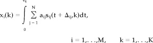(1)

where s_ij indicates spatiotemporal emission of photons that originate from the functional activation j of the subject i with the time delay Δ_ij and its duration τ_ij · a_ij is a weight with which the functional activation j is used in performing the task in subject i and this weight is assumed to be constant during the task. M is the total number of subjects and N is the total number of functional activations. If we focus on the temporal sum of functional activation at the subject i, the integration term of Eq. (1) can be simplified as follows.

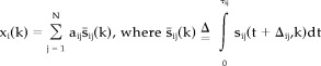(2)

s _ij indicates the accumulated activity of the functional activation j in the i‐th subject. Here, we define the term of “functional component” as the temporally accumulated activity of individual functional activation, which composes total brain activity during a cognitive task. Note that functional component s _ij is a spatial pattern of activation and no longer contains direct temporal information. Nevertheless, we will keep the term “functional” throughout this study because it was derived from the functional activity. Considering most PET studies are composed of multiple trials of the same cognitive task, we can extend Eq. (2) to multiple trials without loss of generality by redefining the functional component as a summation of functional activation across trials.

Figure 1.

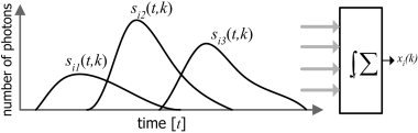
A model of PET measurement at a voxel k of a subject i during a task. The observation x _i (k) is an accumulated number of photons from mixed activations of several functional components of the brain that the voxel k is involved in during a task. Observation x _i (k) is the superimposed activities of functional components at neurons correspondent to the voxel k.

The second assumption of the model is that all subjects homogenously use the common functional components differing only in weights of their usage. According to the homogeneity assumption, functional components in a subject i (s _ij,j=1, …,N) can be replaced with the corresponding common functional components ( _c,c=1, …,N) by changing the order of these components. Then, Eq. (2) can be rewritten as follows. (For simplicity, voxel index k is omitted.)

(3)

where _c= ${}_{\text{O}{}_{\text{i}}\text{(j)}}$=s _ij and c=O_i(j)

_c is a common functional component corresponding to a subject specific component s _ij with a matching function O_i(j). Because O_i(j) connects _c to s _ij and thus to a_ij, reordering a_ij while fixing the sequence of _c will cause equivalent results. Eq. (3) can be rewritten as Eq. (4)

(4)

where _ic = a_{i (c)} and _i(c) = j, _i(O_i(j))=j

If we denote the reordered weight as a_ij and accumulated activity _j as s_j for simplicity, we can rewrite Eq. (4) as Eq. (5) at a specific voxel k in a total of K voxels.

(5)

Note that both the observed activation x_i of subject i and the functional components s_j feature spatial pattern and a_ij is the weight of the spatial pattern (i.e., functional component) being independent of voxel k. The observed brain activations can be interpreted as linear mixtures of common functional components having spatial activations. Eq. (5) can be replaced by the matrix equation of Eq. (6).

(6)

where s=[s₁, …,s_N]^T is composed of the common functional components during the task and is an [N × K] matrix. x represents the observations of all subjects with a matrix size of [M × K] and A is an [M × N] mixing matrix composed of weight elements a_ij as the functional components.

The third assumption is that functional components within a task are independent of each other. The fourth assumption is that each functional component s_j during a task is sparsely localized, i.e., a super Gaussian distribution. The final assumption is that each observation can be represented using the same number of components as the number of observations, i.e., N = M.

The problem of the independent component model (ICM) is then reduced to finding independent functional components (s) and their weights (A) from the observations of all subjects, i.e., x.

ICM for multiple tasks

We can extend this model to the second hypothesis that all subjects share basic functional components common to all tasks and these components are spatially independent of each other. The changes of brain activities due to the task differences arise from the change of the components used, or the change in the weight of the components. This hypothesis can be denoted by the following equation.

(7)

where s ^w=[s${}_{\text{1}}^{\text{w}}$,…,s${}_{\text{N}}^{\text{w}}$]^T represents common functional components involved in the specific task w. x ^w is composed of observations of all subjects during the task w. A ^w is a mixing matrix with weight elements a${}_{\text{ij}}^{\text{w}}$ which vary according to the task w.

If we consider a set S of independent functional components that covers all functional activations of brain, then the set of functional components derived during the task w (s ^w) is a subset of S, i.e., s ^w⊂S and can be subdivided into two subsets, namely, (1) a set of components that are activated independently with the task, including life sustaining activations and basic cognitive activations s ^c and (2) a set of components that are specific to the task s ^ws. The functional component of the task can be denoted as s ^w = s ^c∪s ^ws.

In the ICM model, weight can illustrate the involvement of certain functional components during a task w. If the number of observations is large enough, weights can also generalize the involvement of all functional components in the task, including subject specific components (s ^ws), in the sense that a component that does not exist in one task while existing in another task can be represented by setting its weight to zero. In practice, a limited number of observations and the presence of noise limit the number of components used during a task and the allocating of task specific components.

ICA for ICM

Independent component analysis (ICA), a blind decomposition method, is regarded to be an appropriate method to find independent functional components (s) and their weights (A) from the observations (x) of all subjects in the ICM model.

The application of ICA to ICM is illustrated in Figure 2. From the N independent, but unknown functional components s common to the subject group, brain activities u of each subject emerge by linearly mixing these components. ICA is equivalent to finding a linear transformation matrix W of observations x that makes its outputs u as mutually independent as possible. This can be represented by the following equations.

(8)

where u is an estimate of source functional components s and pu=∏${}_{\mathit{\text{N}}}^{\mathit{\text{i}}\text{=}\mathit{\text{I}}}$ p_i(u_i)

Figure 2.

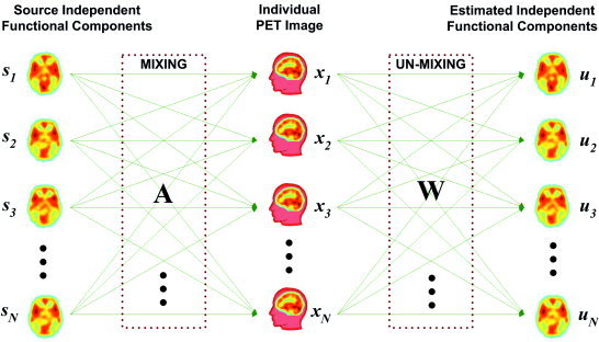
ICA concept in PET decompositions. The basic assumption of ICM is a linear mixture of spatially independent functional components and ICA is an effective tool for unmixing these components. The assumption that all subjects share basic common functional components with subtle variation enables the usage of ICA for finding basic functional components.

Among the various approaches to ICA developed in parallel, we used the infomax learning algorithm proposed by Bell and Sejnowski [1995]. It is a stochastic gradient learning rule derived for a feed‐forward neural network to blindly separate the mixtures of source components. Bell and Sejnowski introduced a nonlinear transformation of source estimates u _i with an invertible monotonic nonlinear function of g, i.e., y _i =g(u _i). By maximizing the joint entropy H(y), they could approximately minimize the mutual information of output components y _i. The mutual information of u _i will be minimized, when the nonlinearity y _i =g(u _i) is the cumulative density function of the source estimates u _i. If a logistic function g(u _i )=tanh(u _i) is chosen as a cumulative density function of super‐Gaussian source, the learning rule reduces to the following natural gradient equation proposed by Amari et al. [1996].

(9)

The basic assumption of the infomax learning algorithm is that the underlying sources are sparsely distributed, i.e., the distribution of each source is super‐Gaussian.

In order to validate ICM and application of ICA, we tested the [¹⁵O]H₂O PET images of multiple subjects with serial task studies and we considered whether the findings of common components across tasks and task‐specific components can support the validity of ICM.

Subjects and Cognitive Tasks

We used PET data, part of which was previously analyzed using the subtraction method by Kim et al. [2002]. We studied 14 healthy, right‐handed Koreans (7 men and 7 women) with the mean ± SD age of 24.8 ± 5.1 years.

The PET data was acquired during four serial tasks with three types of geometric figures (circles, triangles, and squares) as stimuli in random sequence, as is shown in Figure 3. In task 1, the subjects responded whenever the stimuli were presented. In task 2, the subjects watched a list of geometric figures and responded whenever a circle was presented. Task 3 was a sequential object task with a two‐back condition where the subjects were required to continuously monitor a sequence of geometric stimuli and to respond whenever a circle that had been presented before one intervening stimuli was presented again. In task 4, a word was presented in a geometric figure and subjects were requested to respond whenever the name of a flower appeared in a circle, or when the name of an animal name appeared in a rectangle. All words written in Korean were commonly known (e.g., animals: pig, fox, deer, lion, rabbit, mouse, etc.; non‐animals: tree, chair, paper, clock, train, school, etc).

Figure 3.

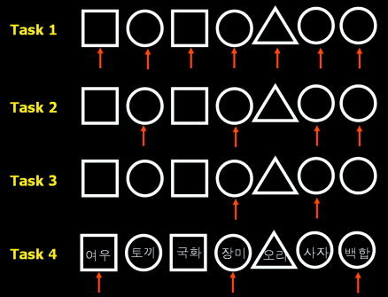
Serial cognitive tasks used for evaluation of ICM. Task 1 is a simple object perception task as a control experiment. Task 2 is an object recognition task where subjects should respond when a circle appears. Task 3 is a two‐back test where a circle appears after the appearance of a circle twice previously. Task 4 is a divided attention task that subjects respond when a flower in a circle and an animal in a rectangle stimuli appear. Arrows indicate the stimuli that subjects should respond. In task 4, the Korean characters in the geometric figure mean “fox/rabbit/chrysanthemum/rose/duck/lion/lily” in that order.

All stimuli consisted of 80 items, including 28 targets. The frequency and distribution of the targets were matched across all tasks. The subjects' responses involved clicking a left mouse button with their right index finger only when the target stimulus was detected.

Imaging Data Acquisition and Preprocessing

All subjects underwent four consecutive PET scans for the four randomly distributed experimental tasks. Scans were obtained using an ECAT EXACT 47 scanner (Siemens‐CTI, Knoxville, TN), which had an intrinsic resolution of 5.2 mm full width at half maximum (FWHM) and simultaneously imaged 47 contiguous transverse planes with a thickness of 3.4 mm for a longitudinal field of view of 16.2 cm. Before the first injection of the tracer, a 7‐min transmission scan was performed for attenuation correction using triple ⁶⁸Ge rod sources. Emission scans during the performance of cognitive tasks started after an intravenous bolus injection of 40–50 mCi of [¹⁵O]H₂O in 5–7 ml saline and continued for 100 s in 20 5‐s frames. Acquired data were reconstructed in a 128 × 128 × 47 matrix with a pixel size of 2.1 × 2.1 × 3.4 mm by means of a filtered back‐projection algorithm employing a Shepp‐Logan filter with a cut‐off frequency of 0.3 cycles/pixel. Based on time‐activity curves, only 12 frames reflecting the 60 s after peak arrival were summed. Injections were repeated at intervals of about 15 min.

Spatial pre‐processing and statistical analysis were performed using SPM 99 (Institute of Neurology, University College of London, UK) [Friston et al., 1995] implemented in Matlab (Mathworks, Newton, MA). All reconstructed images were realigned and transformed into a standard stereotactic anatomical space to remove inter‐subject anatomical variability [Ashburner and Friston, 1999; Talairach and Tournoux, 1988]. Affine transformation was performed in order to determine the 12 optimal parameters to register the brain on a standard PET template. Subtle differences between the transformed image and the template were removed using a nonlinear registration method using the weighted sum of the pre‐defined smooth basis functions used in discrete cosine transformation. Spatially normalized images were smoothed by convolution with an isotropic Gaussian kernel with 16‐mm FWHM in order to increase the signal‐to‐noise ratio and accommodate the subtle variations in anatomical structures.

Independent Component Analysis

Spatial ICA was applied to stereotaxically normalized images of tasks 1, 2, 3, and 4 separately. Note that each task was analyzed independently of the other tasks, which is totally different from the subtraction approach. Regional intensities of all images, masked by the brain mask of SPM99, were normalized proportionally by equating the global mean to 50 ml/min/dl. The infomax learning algorithm using ICA toolbox (available online at http://www.sccn.ucsd.edu/~scott/ica.html) was applied to each task's normalized images, the voxels of which were realigned as a one‐dimensional time series. The learning rate was fixed at 10^‐6. Log likelihood was computed continuously to measure the independency of the output of the network and to determine the optimal repetition time of the training. The components were sorted according to the relative contribution of each component to the original image, which is defined as:

(10)

where W${}_{\text{ij}}^{\text{inv}}$ indicates an element of W^‐1 corresponding t1o the weight of the component j constituting subject i image. x_i(k) is the observation at voxel k of the subject i and u_j(k) is the estimated functional component j at the voxel k.

RESULTS

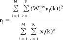
The maximum intensity projection maps of functional components corresponding to experimental tasks are displayed in Figure 4. All map components are illustrated by sagittal view, transverse view, and coronal view, in that order. The left side of the coronal map and the top side of the transverse map indicate the left hemisphere of the brain. The relative contribution of the component, derived by Eq. (10), in composing the brain activation of each subject is displayed at the top‐left of each map with the task number and the order in that task.

Figure 4.

The resultant functional components of PET images during four tasks derived by spatial independent component analysis. The maximum intensity projection maps of functional components corresponding to experimental tasks are displayed. The left map of each figure represents the sagittal section view of maximum intensity and the left side of the map is the posterior brain. The middle map of each figure represents the transverse section view: the top side shows the left brain and the left side shows the posterior brain. The right map of each figure represents the coronal maximum intensity: the left side of the coronal map shows the left side of the brain and the top side shows the top of brain. The relative contribution of the component in composing brain activation of each subject is displayed at the top‐left of each map with the task number and the order in that task. Ten highly contributed components were reordered to similar patterns across the tasks by the correlation coefficient (r) between images of different tasks and visual inspection. Rows 1–3 components show a high correspondence across tasks and rows 4–9 show medium correspondence. The components under the bottom line are unmatched components that we could not match among tasks.

All components of each task, which were derived within the task, were compared with components in the other tasks and re‐ordered according to similar patterns across the tasks. Referencing correlation coefficient(r) between images of different tasks, we categorized images by visual inspection. Rows 1–3 show components with high correspondence (r > 0.5) to the pattern among tasks. Rows 4–9 show components of relatively high correspondence (r > 0.25) among tasks. The remaining components are those that could not be matched with other tasks and are displayed without any relation to each other's task.

The first row component is composed of activation in the bilateral cerebellums. The second row component is located in the sensory and motor areas and the third component is located in the supplementary motor area. The contribution rates of the three components are almost the same throughout the tasks. The fourth component covers mainly the occipital lobe and a small portion of the parietal lobe. The fifth component seems to correspond to the fusiform gyrus, including ventral occipito‐temporal pathway. Activations in basal ganglia seem to appear in the fifth component of tasks 1 and 2. The third component in task 3 corresponds to both the fourth and the fifth components of the other tasks with relatively high correlation. The mean usage of this component in task 3 is 39%, which is a similar value to that obtained by adding the fourth and fifth components in the other tasks. The sixth component is mainly located bilaterally at orbito‐frontal lobes and shows somewhat different patterns by tasks. The sixth component of both tasks 2 and 3 is distributed mainly in the frontal area including dorso‐lateral prefrontal, orbito‐frontal and anterior cingulate cortex. The seventh component seems to correspond to lingual gyrus.

The unmatched three components in task 1 are composed of the left frontal cortex, right orbito‐frontal cortex, and both anterior temporal regions. The unmatched three components in task 3 are mainly located in the prefrontal areas (from the first to third components). The last unmatched component in task 3 shows bilateral parietal involvement. The first unmatched component of task 4 is mainly located in the occipital, left temporal and right parietal lobes. The second unmatched component of task 4 is located in the left dorso‐lateral prefrontal and left temporal regions. The right dorso‐lateral prefrontal area is found in the third unmatched component of task 4.

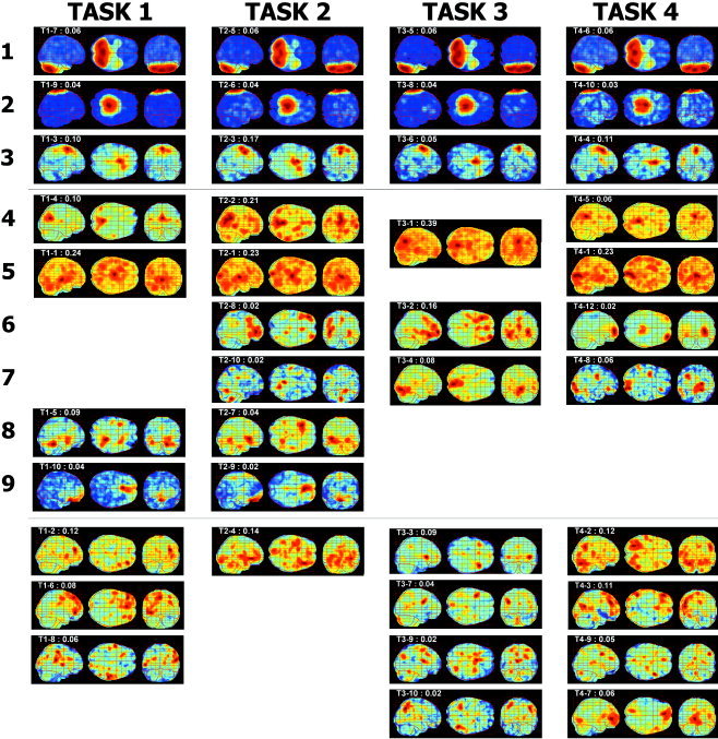
Figure 5 shows an example of mixing matrixes A of Eq. (6) in task 2 (Fig. 5a) and task 3 (Fig. 5b). Mixing matrices provides information on the weight of the component usage according to subjects and tasks. Components were ordered according to the relative contribution to the original image using Eq. (10) from high to low values. Color values indicate strengths of weights, i.e., strengths of the usage of each component in the subjects. First, components of task 2 and task 3 correspond to the fifth row of task 2 and the fourth row of task 3, respectively, in Figure 4. From the mixing matrix A, we can understand how each component is used for a subject to perform a task. For example, subject 11 had the highest usage of component 1 (i.e., the fifth row of task 2, ventral occipito‐temporal pathway and basal ganglia) in task 2, followed by Subject 5, etc. Subject 11 thus used the brain areas identified by component 1 strongly for task 2. In general, the component usage was found to be homogenous throughout subjects except for some minor differences. Figure 5 also provides task‐specific information; for example, most high‐contribution components were evenly involved in task 2 while task 3 seemed to require focused usage of component 1 (i.e., the fourth component of task 3 in Fig. 4) compared to task 2.

Figure 5.

Weight usage of subjects at task 2 and task 3. The weights of functional components according to subjects are displayed during task 2 (a) and task 3 (b) in order to illustrate the homogenous usage of weights with little variation. Components were ordered from high relative contribution to low contribution to the original image. The color scale indicates strengths of weights, i.e., strengths of the usage of each component in the subjects.

Figure 6 shows the mutual information between all components of the four tasks, which was derived from the algorithm of Moddemeijer [1989]. The total number of components derived from the four tasks was 56. Each task has a block of 14 components. The diagonal elements with the highest values indicate mutual information between self‐components. A diagonal block indicates mutual information within tasks while an off‐diagonal block indicates mutual information across tasks. Low values in off‐diagonal elements show independence between components within a task and across tasks. Mutual information between components within a task is generally lower than that of between tasks because ICA was applied to images within tasks. We can see several relatively high‐value spots in off‐diagonal elements, which indicate the existence of similar components across tasks. They are correspondent to row 1–3 components.

Figure 6.

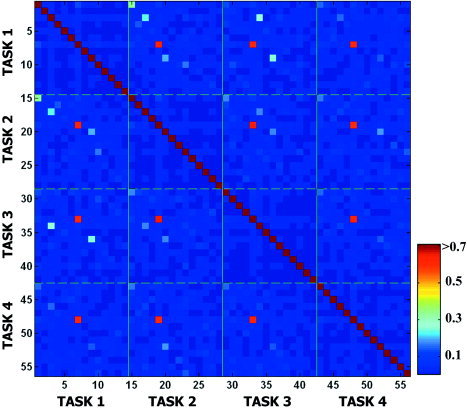
Mutual information between all components derived throughout four tasks. The mutual information between all components of the four tasks, in total 56 components, was displayed. The color bar indicates the strength of mutual information between components. The diagonal elements indicate mutual information between self‐components. A diagonal block indicates mutual information within tasks while an off‐diagonal block indicates mutual information across tasks.

We also applied an extended infomax algorithm in order to validate the ICA algorithm in the ICM model, but the mean mutual information of each independent component was not found to be as significant compared to that which was derived from the general infomax algorithm. Thus, we accepted the result of the general infomax algorithm, which follows the model's assumption.

DISCUSSION

Independent Functional Components Across Subjects and Tasks

Basic functional activations, including sensory and motor functions and visual analysis that perceive the shape passively, may be activated throughout the tasks. Sustained attention and shape recognition are possibly involved in all tasks, even though the activation is thought to be weak in task 1 when compared with other tasks. Working memory is thought to be involved in both the two‐back task (task 3) and the divided attention task (task 4) but the type of involvement is believed to be different. Semantic processes of categorization and divided attention are also considered to be involved in task 4. The following interpretation of the results is largely based on the extensive review of Cabeza and Nyberg [2000].

Row 1 to 5 components show similar activation patterns but little difference in contributions to the tasks and indicate the components common to the four tasks. The first row component is mainly located in bilateral cerebellums that are known to play an important role in cognition, such as motor preparation, sensory acquisition, timing [Ivry, 1997], and attention/anticipation [Akshoomoff et al., 1997]. The second row component (sensory and motor area) and the third row component (supplementary motor area) may be involved in sensory‐ and motor‐related activity, relevant or irrelevant to the tasks. We concluded that these three components may be related to the primary brain activities, including basic cognition.

The fourth component that covers the occipital lobe may be related to primary visual perception. The fifth component may correspond to the visual recognition of objects, which is related with activations in the ventral pathway [Ungerleider and Mishkin, 1982]. Basal ganglia seems to be highly involved in this component of tasks 1 and 2 and seems to show relatively decreased activation in tasks 3 and 4 as higher levels of cognitive processing is required.

The unmatched components in task 3 are thought to be related with working memory, which is mediated by the dorsolateral prefrontal cortex (DLPFC) and its reciprocal cortical connections with other brain regions, such as the cingulate, temporal, and parietal cortices [Courtney et al., 1998].

The first and second unmatched components of task 4 show left lateralized activations and may be related with language and semantic processes, especially written word recognition and categorization. Left middle temporal gyrus (BA 21) and bilateral occipito‐temporal regions (BA 37) are known to be involved in semantic retrieval. The third component may be related to spatial working memory.

To summarize the above results, we found it plausible that ICM helps explain the brain activations of subjects during real experimental tasks. We do not disclaim that the above interpretations may contain over‐interpretations, in part. The exact meaning for each component still remains for further study. Even though we could not match all functional components to cognitive processes precisely and found some limitations, ICA is regarded to be effective considering that it decomposes functional components blindly from images of multiple subjects without any a priori constraint or control experiment.

How Does ICM Describe Brain Activation?

The major assumptions used in ICM are partly supported by the work of McKeown et al. [McKeown et al. 1998], who tried to validate the ICA assumptions on fMRI, and who showed the plausibility of the constant linear mixing of components sparsely distributed throughout the brain with the same number of components contained in the data as the number of channels (in our case, number of subjects). The assumption that multiple subjects share common cognitive components can be considered acceptable in view of the fact that most within‐group experiments explore subject‐independent cognitive processes, i.e., common components across subjects.

The idea that subjects share basic functional components with subtle variations is the cue to exploring the spatial pattern of the functional components expected to exist in the task. The model explains the different brain activations of subjects by changing the weights of common independent functional components, which are assumed to be fixed during the task. The weight of a certain component remained within a limited range for all of our subjects, which implies a relatively homogenous involvement of functional components among subjects. Spatial pattern of each functional component represents spatially synchronized activation that has the same origin across voxels, i.e., the same functional process, and it implies a functional association analogous to the “functional connectivity,” which has the meaning of temporal inter‐correlation.

It should be noted that ICM is an indirect way to explore functional components using subject variability. ICA can only extract the spatially independent components that recruit distinct brain areas that vary significantly from subject to subject in performing a task. A spatial component that has the same involvement in a task from subject to subject cannot be extracted by ICA. However, this might not be the case in real data since the subject‐variability of the involvement of any brain region in performing any task always exists.

Independent Functional Components of ICM and Real Cognitive Components

A question remains about the relationship between the independent functional components in the model and real cognitive components of the brain. Through our experiments, we found a high correspondence between specific cognitive processes and functional components. However, for some functional components, two or more cognitive components seem to be mixed, while others seem to be divided into two or more functional components.

The errors of decomposition may be derived partly from noise effects and the imperfectness of ICA algorithms in solving ICM in addition to modeling errors that underlying assumptions of ICM may not fit the characteristics of the real data sufficiently, such as nonlinear nature of some cognitive processes. In the application of ICA to ICM, no explicit noise model is used; thus, it is assumed that noise is distributed among one or more of the components [McKeown and Sejnowski, 1998]. Accordingly, noise may be contained in the derived components in part and may degrade the decomposition. Also, the ICA technique is still under development and the conventional ICA algorithm does not always give a perfect solution to the ICM model. Lack of knowledge about the number of functional components involved in a task can also deteriorate the separation. For example, when the number of cognitive processes is more than that of subjects, the ICA learning algorithm may derive under‐complete separation of independent components, while in the reverse case, the ICA algorithm may derive over‐complete separation of independent components even if the weights of extra components should be near zero.

As was discussed in the paper by McKeown et al. [1998b], we cannot disregard the limitations of ICA and ICM in decomposing the nonlinear interaction between cognitive functions [Friston et al., 1996; Price and Friston, 1997]. Basically, ICM assumes that each functional component is linearly independent, and, therefore, a nonlinear interaction may be decomposed into two or more linear components. Nonlinear interaction can be illustrated either by nonlinear changes of a component weight due to a nonlinear modulator or by a new linear component generated by a nonlinear modulator that differs from the existing functional components in ICM.

As a data‐driven explorative approach, ICM cannot be easily validated by statistical methods due to the different goals and approaches of the two methods. Statistical methods based on subtraction scheme have been used to investigate mainly functional localization by testing pre‐determined hypotheses and have proven to be a matchless tool in the neuroimaging field. Using the subtraction scheme, several powerful methodologies from pure insertion and factorial analysis to conjunctional analysis have been established during the last decades. Interpretation of ICA for ICM in this study is also based on the previous findings of the subtraction method. However, the subtraction method mainly gives information on additive components, and, therefore, requires a control task for contrasting experimental tasks. In addition, it does not provide much information on the functional connection between brain regions. In other words, in order to be statistically clear, the method sacrifices the integration of functional components. Meanwhile, ICM can give some clues concerning functional association in addition to function segregation from a set of cross‐sectional images. ICM and ICA can provide additional information on what types of functional components are involved during tasks, which the subtraction method cannot provide. Moreover, the subtraction method can possibly be explained by ICM based on changes in component weight.

Concluding Remarks

ICM starts from homogeneous characteristics across subjects within a group. Therefore, ICM can be extended to exploring group differences and may be an efficient tool for characterizing disease‐specific brain activations.

In summary, we have mathematically derived an independent component model (ICM) to illustrate subject variability and the task differences of cognitive functions. Also, by serial task design, we partly confirmed the validity of our model.

REFERENCES

- Akshoomoff NA, Courchesne E, Townsend J (1997): Attention coordination and anticipatory control. Int Rev Neurobiol 41: 575–598. [DOI] [PubMed] [Google Scholar]
- Amari S, Cichocki A, Yang HH. (1996): A new learning algorithm for blind source separation In: Advance in neural information processing systems 8 Cambridge, MA: MIT Press, p 757–763. [Google Scholar]
- Ashburner J, Friston KJ (1999): Nonlinear spatial normalization using basis functions. Hum Brain Mapp 7: 254–266. [DOI] [PMC free article] [PubMed] [Google Scholar]
- Bell AJ, Sejnowski TJ (1995): An information‐maximization approach to blind separation and blind deconvolution. Neural Comput 7: 1129–1159. [DOI] [PubMed] [Google Scholar]
- Cabeza R, Nyberg L (2000): Imaging cognition II: An empirical review of 275 PET and fMRI studies. J Cogn Neurosci 12: 1–47. [DOI] [PubMed] [Google Scholar]
- Courtney SM, Petit L, Maisog JM, Ungerleider LG, Haxby JV (1998): An area specialized for spatial working memory in human frontal cortex. Science 279: 1347–1351. [DOI] [PubMed] [Google Scholar]
- Friston KJ, Liddle PF, Frith CD, Hirsch SR, Frackowiak RS (1992): The left medial temporal region and schizophrenia. A PET study. Brain 115: 367–382. [DOI] [PubMed] [Google Scholar]
- Friston KJ, Frith CD, Liddle PF, Frackowiak RS (1993): Functional connectivity: the principal‐component analysis of large [PET) data sets. J Cereb Blood Flow Metab 13: 5–14. [DOI] [PubMed] [Google Scholar]
- Friston KJ, Holmes AP, Worsley KJ, Poline JB, Frith CD, Frackowiak RS (1995): Statistical parametric maps in functional imaging: a general linear approach. Hum Brain Mapp 2: 189–210. [Google Scholar]
- Friston KJ, Price CJ, Fletcher P, Moore C, Frackowiak RS, Dolan RJ (1996): The trouble with cognitive subtraction. Neuroimage 4: 97–104. [DOI] [PubMed] [Google Scholar]
- Horwitz B (1990): Simulating functional interactions in the brain: a model for examining correlations between regional cerebral metabolic rates. Int J Biomed Comput 26: 149–170. [DOI] [PubMed] [Google Scholar]
- Horwitz B (1991): Functional interactions in the brain: use of correlations between regional metabolic rates. J Cereb Blood Flow Metab 11: A114–120. [DOI] [PubMed] [Google Scholar]
- Hyvärinen A, Karhunen J, Oja E (2001): Independent component analysis. New York: John Wiley & Sons, Inc. [Google Scholar]
- Ivry R (1997): Cerebellar timing systems. Int Rev Neurobiol 41: 555–573. [PubMed] [Google Scholar]
- Kim JJ, Kim MS, Lee JS, Lee DS, Lee MC, Kwon JS (2002): Dissociation of working memory processing associated with native and second languages: PET investigation. Neuroimage 15: 879–891 [DOI] [PubMed] [Google Scholar]
- Lee T‐W (1998): Independent component analysis theory and applications. Boston: Kluwer Academic Publishers. [Google Scholar]
- Makeig S, Jung TP, Bell AJ, Ghahremani D, Sejnowski TJ (1997): Blind separation of auditory event‐related brain responses into independent components. Proc Natl Acad Sci USA 94: 10979–10984. [DOI] [PMC free article] [PubMed] [Google Scholar]
- McKeown MJ, Sejnowski TJ (1998): Independent component analysis of fMRI data: examining the assumptions. Hum Brain Mapp 6: 368–372. [DOI] [PMC free article] [PubMed] [Google Scholar]
- McKeown MJ, Jung TP, Makeig S, Brown G, Kindermann SS, Lee TW, Sejnowski TJ (1998a): Spatially independent activity patterns in functional MRI data during the stroop color‐naming task. Proc Natl Acad Sci U S A 95: 803–810. [DOI] [PMC free article] [PubMed] [Google Scholar]
- McKeown MJ, Makeig S, Brown GG, Jung TP, Kindermann SS, Bell AJ, Sejnowski TJ (1998b): Analysis of fMRI data by blind separation into independent spatial components. Hum Brain Mapp 6: 160–188. [DOI] [PMC free article] [PubMed] [Google Scholar]
- Moddemeijer R (1989): On estimation of entropy and mutual Information of continuous distributions. Signal Process 16: 233–246. [Google Scholar]
- Moeller JR, Strother SC (1991): A regional covariance approach to the analysis of functional patterns in positron emission tomographic data. J Cereb Blood Flow Metab 11: A121–135. [DOI] [PubMed] [Google Scholar]
- Price CJ, Friston KJ (1997): Cognitive conjunction: a new approach to brain activation experiments. Neuroimage 5: 261–270. [DOI] [PubMed] [Google Scholar]
- Talairach J, Tournoux P (1988): Co‐planar stereotaxic atlas of the human brain. New York: Thieme. [Google Scholar]
- Ungerleider LG, Mishkin M (1982): Two cortical visual systems In: Ingle DJ, Goodale MA, Mansfield RJW, editors. Analysis of visual behavior. Cambridge, MA: MIT Press; p 549–589. [Google Scholar]