Characterizing instantaneous phase relationships in whole‐brain fMRI activation data

Abstract

Typically, fMRI data is processed in the time domain with linear methods such as regression and correlation analysis. We propose that the theory of phase synchronization may be used to more completely understand the dynamics of interacting systems, and can be applied to fMRI data as a novel method of detecting activation. Generalized synchronization is a phenomenon that occurs when there is a nonlinear functional relationship present between two or more coupled, oscillatory systems, whereas phase synchronization is defined as the locking of the phases while the amplitudes may vary. In this study, we developed an application of phase synchronization analysis that is appropriate for fMRI data, in which the phase locking condition is investigated between a voxel time series and the reference function of the task performed. A synchronization index is calculated to quantify the level of phase locking, and a nonparametric permutation test is used to determine the statistical significance of the results. We performed the phase synchronization analysis on the data from five volunteers for an event‐related finger‐tapping task. Functional maps were created that provide information on the interrelations between the instantaneous phases of the reference function and the voxel time series in a whole‐brain fMRI activation data set. We conclude that this method of analysis is useful for revealing additional information on the complex nature of the fMRI time series. Hum. Brain Mapping 16:71–80, 2002. © 2002 Wiley‐Liss, Inc.

INTRODUCTION

The study of nonlinear dynamics involves the investigation of systems in which the output is not proportional to the input, that is, these systems respond nonlinearly to a perturbation. We may wish to explore the working relationships of such systems or subsystems and are primarily interested in the interactions of these systems. Synchronization is a nonlinear phenomenon that is of much relevance when studying the intricate dynamics between oscillators that are either weakly coupled or driven by an external force [Hayashi, 1964; Minorsky, 1974].

The definition of synchronization is not widely agreed upon; however, it is generally acknowledged that synchronization occurs when there exists a functional relationship between subsystems. The occurrence of synchronization has been observed in many studies of man‐made systems [Blekhman, 1988] and in nature, such as in the analysis of the effects of light on neuroendocrine circadian rhythms [Aschoff et al., 1982], the simultaneous recordings of breathing and gait in running mammals [Bramble and Carrier, 1983], local field potential oscillations in the orientation columns of the feline visual cortex [Gray and Singer, 1989], in vitro analysis of the inferior olivary neurons of the olivo‐cerebellar system [Makarenko and Llinas, 1998], investigation of brain activity during pathological tremor with magnetoencephalography (MEG) and electromyogram (EMG) recordings [Tass et al., 1998], electrocardiogram (ECG) and thermistor readings of the human cardiorespiratory system [Rosenblum et al., 1998; Schafer et al., 1999], LFP data from human intracortical recordings [Lachaux et al., 1999], extracellular recordings in the electrosensitive cells in paddlefish [Neiman et al., 1999], and near‐infrared spectroscopy (NIRS) of motor cortex hemodynamics [Toronov et al., 2000].

The classical theory of synchronization has been thoroughly developed with respect to periodic signals, and it was determined that phase locking and frequency locking are equivalent in these systems [Hayashi, 1964; Pikovsky et al., 2000]. Classically, in periodic oscillators, phase synchronization is defined as the locking of the phases of the two systems whereas their amplitudes may vary. That is, two instantaneous phase signals, θ _i(t) and θ _j(t), are in synchrony if the phase‐locking condition is met:

(1)

This condition poses no restriction on the amplitudes of the times series under investigation [Tass et al., 1998].

Recent studies have increased our understanding of synchronization in non‐periodic, noisy, or chaotic systems, and have shown that it is possible to detect synchronization in these systems also [Rosenblum et al., 1996, 1997]. In noisy systems, phase synchronization is a transient process, as signals randomly find themselves in and out of synchrony due to the presence of noise. In this case, phase and frequency locking may no longer be equivalent [Schafer et al., 1999]. Thus, investigation of synchronization phenomena in noisy systems requires a quantitative analysis of the instantaneous phase signals. Phase synchronization is similarly defined in chaotic and noisy systems, and it is this property that allows both types of systems to be analyzed in the same manner [Tass et al., 1998]. If the goal is to analyze the instantaneous phases in experimental data, it is irrelevant whether the oscillations under consideration are chaotic or noisy, as the method remains the same for either case [Pikovsky et al., 2000].

To detect the presence of synchronization in coupled systems from experimental time series data, there are two assumptions that must be made. First, the time series in question must be narrow‐banded signals to obtain estimates of the instantaneous phases. Second, the time series must arise from systems that are self‐sustained oscillators. That is, the systems must generate their own rhythms. If these assumptions are justified, then it is possible to detect phase synchronization in interacting systems by the analysis of the instantaneous phases. If these are not reasonable assumptions, no conclusions concerning the occurrence of the nonlinear phenomenon of phase synchronization may be made. If this is the case, however, analysis of the instantaneous phases remains a valid method of analyzing time series to characterize a specific interrelation between phases [Pikovsky et al., 2000].

Typically, fMRI data is processed in the time domain with linear methods such as regression and correlation analysis. We propose that investigating the relationships between the instantaneous phases of the reference function and the voxel time series in fMRI data will provide additional information on the dynamics of functional activation. By analyzing the instantaneous phases, specific dependencies between subsystems may be uncovered in situations where the original time series may be completely uncorrelated. As our analysis involves the instantaneous phase of the reference function, we are not assuming that our oscillators are self‐sustained oscillators. Therefore, our aim was not to detect the occurrence of phase synchronization, but rather to detect an interrelation between the instantaneous phases of the reference function and all voxel time series. That is, our goal was to detect a relationship between the phases in experimental fMRI data from the nonlinear dynamics perspective where the true signal may be masked by noise. The further purpose of this study was to detect this type of relationship in the cortical areas associated with fMRI motor activation in an event‐related paradigm.

MATERIALS AND METHODS

Data were acquired for this study on a clinical 1.5 T GE Signa LX scanner (General Electric, Waukesha, WI) equipped with high‐speed gradients for whole‐body EPI. A preliminary anatomical scan was performed to acquire a set of high‐resolution SPGR images for functional image coregistration. Gradient‐recalled echo single‐shot EPI images were acquired at 22 coronal slice locations: slice thickness 7 mm; gap spacing 1 mm; flip angle 90°; FOV 24 cm × 24 cm; TE 40 msec; TR 2,000 msec; and a 64 × 64 imaging matrix.

Five normal volunteers, between 20 and 35 years of age, with no history of neurological disorder participated in this study after consent was obtained in accordance with institutional policy. Data was collected using an event‐related motor task paradigm, which was composed of a self‐paced alternate‐hand finger tapping exercise. In this task, visual cues for right‐ and left‐hand tapping were presented randomly in 2‐sec blocks. One hundred fifty data points were collected for each voxel. Analysis began with the reconstruction of the raw EPI data into spatially localized time series of signal intensity vs. time for each voxel. The slices were time corrected, and a 3‐point Hanning filter was applied for temporal smoothing of the data. The first four images of each slice location were disregarded due to incomplete saturation of the signal. The analysis of phases presented here was written in Matlab (Mathworks, Natick, MA).

Hilbert Transform

Determination of a relationship between phases using the theory of phase synchronization requires the calculation of the instantaneous phase signal for each voxel time series. Lachaux et al. [1999] convolved their data with a complex Gabor wavelet to extract the phase information. This can also be accomplished by use of the Hilbert transform. Previously, the Hilbert transform has been used in fMRI as a method of estimating the hemodynamic delay response [Saad et al., 2001].

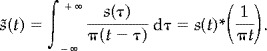
For a real‐valued time‐domain signal s(t), the Hilbert transform, s̃(t), is defined as the convolution integral of s(t) and (1/πt). That is,

(2)

To avoid the complexities of computation associated with the poles in the above integral, we note that the Fourier transform of s̃(t) is S̃(f), and can be computed through use of the convolution property of Fourier theory:

(3)

where S(f) is the Fourier transform of our signal s(t), sgn(f) is the signum function, and i · sgn(f) is the Fourier transform of 1/πt [Bendat and Piersol, 2000]. In the calculation of the instantaneous phase signal of s(t), it is necessary to introduce the concept of the analytic signal [Gabor, 1946]. A real signal and its Hilbert transform are used to form a new complex signal, z(t), which is the analytic signal corresponding to the real signal. The analytic signal, z(t), has no negative‐frequency components, and is defined as:

(4)

where A(t), the envelope signal of s(t), and θ(t), the instantaneous phase signal of s(t), are uniquely defined [Rosenblum et al., 1998; Schafer et al., 1999]. Then the Fourier transform of z(t) is Z(f):

(5)

Thus, by starting with the signal, s(t), we calculate the Fourier transform, S(f), multiply positive frequencies by two and negative frequencies by zero, and take the inverse Fourier transform to obtain z(t). The instantaneous phase signal is then defined as:

(6)

Phase Difference Signal

To investigate the phase interrelations in fMRI data between a voxel with time series x _i(t _k) and a reference function x _j(t _k), we first calculate the instantaneous phase signal of these time series, θ _i(t _k) and θ _j(t _k), respectively. The phase locking condition [Tass et al., 1998] is satisfied if the phase difference signal

(7)

oscillates around a constant value.

There is no accepted method of determining n and m, and therefore, many authors choose these values by trial and error [Rosenblum et al., 1998; Schafer et al., 1999; Tass et al., 1998; Toronov et al., 2000]. This technique works well when applied to data from MEG, ECG, and NIRS studies, as they are not comprised of an excessively large number of time series. Due to the large number of time series obtained in an fMRI study; however, this is an impractical approach. Thus, n was assigned the value of one, and a least‐squares fitting was performed to determine the value of m for each phase difference signal, θ _i,j(t _k), in the brain, so as to minimize the difference between the two signals. The phase difference signal was determined by subtracting the instantaneous phase signal of the voxel under investigation from the instantaneous phase signal of the reference function of the task performed according to the above equation. The reference function was created by convolving the stimulus time series (ones for tapping, zeros for resting) with a hemodynamic response function. This hemodynamic response function consisted of two gamma functions shifted 2 sec apart. The procedure for determining the phase difference signal was repeated for all voxels in the brain. Previous studies have determined the presence of phase synchronization by visual inspection of the instantaneous phase information [Bramble and Carrier, 1983; Rosenblum et al., 1996, 1998; Schafer et al., 1999]. This not a sufficient means of characterizing a relationship between instantaneous phases, and it is necessary to formulate a statistical procedure to quantify the strength of this relationship.

Synchronization Index

In synchronization theory, the degree of phase synchronization is determined by analysis of the distribution of the phase difference signal, also called the relative phase distribution [Stratonovich, 1963]. The relative phase distribution for two time series that are phase‐locked is a peaked distribution, due to the fact that in noisy systems the relative phase signal fluctuates around some preferred value. Thus, quantification of phase synchronization deals with the analysis of the distribution of the relative phase. Even though our goal was not to detect the presence of phase synchronization, we chose to proceed with our analysis of the relative phases based on the theory of phase synchronization. Our chosen test statistic is based on the entropy [Shannon and Weaver, 1949],

(8)

where p _i is the probability mass of the phase difference signal, θ _i,j(t _k), over N bins. It is easily shown that the maximum entropy, S _max = ln(N), characterizes a uniform probability distribution. This maximum entropy aids us in normalizing what Tass et al. [1998] define to be the synchronization index:

(9)

The values of η range from zero to one, where zero corresponds to no synchronization, or a uniform distribution, and one corresponds to a perfect synchronization, or a Dirac delta distribution [Tass et al., 1998].

Nonparametric Permutation Tests

To make a valid assessment of the statistical significance of the results obtained while minimizing Type I error, it is necessary to develop an accurate procedure for calculating the significance levels of the synchronization indices. Since the distribution of the index is unknown, we must proceed with a nonparametric approach. For this analysis, we have chosen the permutation test [Nichols and Holmes, 2002], a test that is computationally expensive, but also very flexible. There are two different methods of applying permutation theory to fMRI data to obtain the null distribution of the test statistic. One is to permute the labels of the scans of the stimulus function, which is sometimes called a randomization test. The other method is based on repeated random resampling of the observed data. This can be justified by accounting for the temporal autocorrelations present in the data or orthogonal transformation to another domain [Bullmore et al., 2001].

In this study, we have chosen to proceed with the randomization test, which we will refer to as the permutation test, for simplicity. The use of this test is justified by the initial randomization of the presentation order of the task. By choosing a randomized presentation order of the task, we have avoided confounding effects associated with the hemodynamic response. This method of statistical inference may be applied to non‐randomized tasks only when an effort is made to model the temporal autocorrelations present in the fMRI time series [Nichols and Holmes, 2002].

The null hypothesis is concerned only with the data acquired, and states that the intensity of each image collected will be unchanged, regardless of the presentation order. To test whether there is evidence against the null hypothesis, we first look at the stimulus time series. Assuming that the null hypothesis is true, then if the stimulus time series is permuted with all possible orderings equally probable, the resulting statistics will be equal to those obtained for the actual stimulus time series. That is, the set of test statistic values associated with each permutation are all equally probable. When the values of the test statistic are computed for all possible permutations of the stimulus time series, we have the permutation distribution of our test statistic for one voxel. Permutation theory states that under the null hypothesis, this permutation distribution is the sampling distribution of our synchronization index. The critical value of the index for a given significance level may then be obtained directly from this distribution [Nichols and Holmes, 2002].

For the case of calculating the significance level, α, for a whole brain image of synchronization indices, we encounter the multiple comparison problem that accompanies standard voxel‐by‐voxel testing. Our approach to this issue was to consider a maximal statistic. First, we performed the above computations on all voxels for a single permutation and recorded the maximum value obtained from these synchronization indices. That process was repeated for all permutations under consideration to obtain a distribution of the maximum values of the index, for all voxels and all permutations. This distribution is the permutation distribution for the maximal statistic [Nichols and Holmes, 2002].

The omnibus null hypothesis that all null hypotheses for all voxels are true is rejected for a given significance level if the maximal statistic for the actual stimulus time series is in the top 100α% of this distribution. This method requires that the permutation distributions are similar across all voxels. There are three reasons that we will assume similar voxel permutation distributions for all subjects in this study. First, verification of this assumption is extremely computationally expensive. Second, previous research [Holmes et al., 1996] indicates that the loss of power associated with variation among voxel permutation distributions is negligible. Third, our test statistic is normalized. Thus, this method of statistical inference accounts for the multiple comparisons problem associated with testing all voxels in a dataset simultaneously [Nichols and Holmes, 2002].

For a functional imaging scan of 150 time points, there are 150! ways of permuting the stimulus time series, assuming full exchangeability. Including all permutations in the calculations is not a practical method of determining the significance level of the statistical image due to the number of computations. It is acceptable to test a subsample of these permutations comprised of 1,000 permutations [Edgington, 1995], thereby performing an approximate permutation test. In this case, the actual permutation of the stimulus time series should be included in the subsample. We determined the null distribution for the maximal synchronization index on a subject‐by‐subject basis, for both the right‐ and left‐hand stimulus time series. It is in this manner that all functional images were assessed for significance at a level α = 0.05.

Surrogate Data

We wished to perform the analysis of the relative phases on simulated data to test the efficacy and reliability of this method. Previous studies have indicated that this is a complicated issue [Rosenblum et al., 1998; Schafer et al., 1999]. In the field of nonlinear dynamics, results are often validated using the surrogate data technique. The first step of this procedure is to compute the test statistic with the experimentally obtained data. Then a surrogate data set is constructed in which certain properties of the original signal are preserved. The test statistic is again calculated using the surrogate data, and compared to the results of the observed data to determine if there are any differences [Palus and Hoyer, 1998; Schreiber and Schmitz, 2000]. We have applied this technique with the goal of determining if the relation between phases that we have detected is randomly occurring or if it is due to a feature of the experimental data.

The most crucial step of surrogate data testing is constructing the surrogates. Frequently, this is done by randomization of the Fourier phases. This is not a suitable technique in validating the results of the analysis presented here because any manipulation of the Fourier phases would surely alter the properties of the signal that are of the most interest to our analysis. Wavelet resampling is better suited as a method of generating surrogate data in our case. Studies have shown that the power spectra of scans conducted under resting conditions exhibits 1/f‐characteristics [Aguirre et al., 1997; Zarahn et al., 1997], and that fractional Brownian motion may be used as a model for 1/f noises [Mandelbrot and Van Ness, 1968]. Resampling via wavelet decomposition is the preferable method for testing fMRI data as it preserves the second order stochastic properties and successfully decorrelates fractional Brownian motion [Bullmore et al., 2001; Percival, 1999].

We chose to follow the algorithm proposed by Bullmore et al. [2001] to construct our surrogates. In this algorithm, a level five decomposition was performed for a single time series in one data set using the fourth‐order Daubechies wavelet. This particular wavelet was chosen to maximize the decorrelation between the wavelet coefficients [Flandrin, 1992; Tewfik and Kim, 1992]. The wavelet coefficients were randomly permuted without replacement at each level of detail. The inverse wavelet transform was performed to obtain the wavelet‐resampled time series. This procedure was repeated for every time series in the brain for one volunteer and these resampled time series comprised the surrogate data set [Bullmore et al., 2001]. The synchronization index was then computed for each voxel in the surrogate data. Studies have indicated that it is satisfactory to test 19 or 39 surrogate data sets [Prichard and Theiler, 1994; Schreiber and Schmitz, 2000]; however, we chose to construct and analyze 99 surrogates. Thus one hundred synchronization indices were computed at each voxel, including those obtained from the experimental data. To correct for multiple comparisons, we recorded the maximum index for each permutation of the wavelet coefficients. These maximum synchronization indices were used to compare the significance of the results of the experimentally obtained data to the surrogate data. This surrogate data technique of validating the results of the analysis of the relative phases was performed on each of all five volunteers.

RESULTS

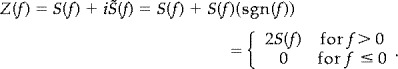
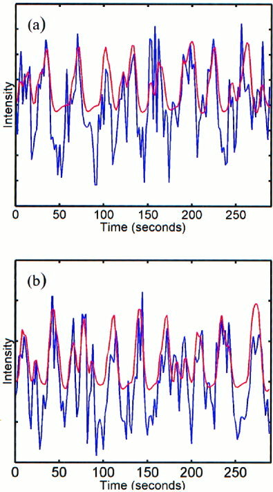
The analysis of the relative phases was completed individually for all five volunteers for the left‐ and right‐hand reference functions of the event‐related finger‐tapping task. Functional maps were created for the task performed by each volunteer, signifying the interrelation between the instantaneous phases of the reference function and all voxel time series during activation of the motor cortex. Figure 1a,b show the reference functions in red for the task performed and sample time series in blue. These time series were selected as those having the highest synchronization index with the reference function. The time series in Figure 1a corresponds to a voxel time series obtained in the left motor cortex, whereas the time series in Figure 1b corresponds to a voxel time series obtained in the right motor cortex. Histograms of the relative phase distribution for right‐hand tapping are shown in Figure 2. The peaked distribution above reveals the strong dependency between the instantaneous phases of the reference function and a voxel time series in the left motor cortex, whereas the more uniform distribution below reveals the absence of any such relationship between the phases of the reference function and an arbitrarily chosen voxel in the frontal lobe. Figure 3 displays the results of the analysis of the relative phases as functional maps (P < 0.05) for both right‐hand (η > 0. 0840) and left‐hand (η > 0. 0850) finger tapping for one volunteer. All of the maps created from the data of the five volunteers consisted of small, localized activation of the primary motor cortex. For comparison, Figure 4 shows the results obtained when the same data analyzed in Figure 3 is analyzed in a more conventional fashion using the SPM'99 software package (Wellcome Institute of Cognitive Neurology, London, England). In this analysis, a method based on the theory of Gaussian fields was used to correct for multiple comparisons (P < 0.05). The same hemodynamic response function was used in the SPM analysis and the relative phase analysis. Results from all five volunteers of the surrogate data testing revealed that the synchronization indices of the relative phase analysis on the observed data set were significantly different from those computed on the wavelet‐resampled surrogate data sets (P < 0.001).

Figure 1.

Reference function in red with a sample time series in blue for right‐hand tapping (a) and left‐hand tapping (b).

Figure 2.

Histograms of the relative phase distributions for right‐hand tapping corresponding to the instantaneous phases of the reference function and a voxel when a significant interrelation is present (a) and when this interrelation is absent (b).

Figure 3.

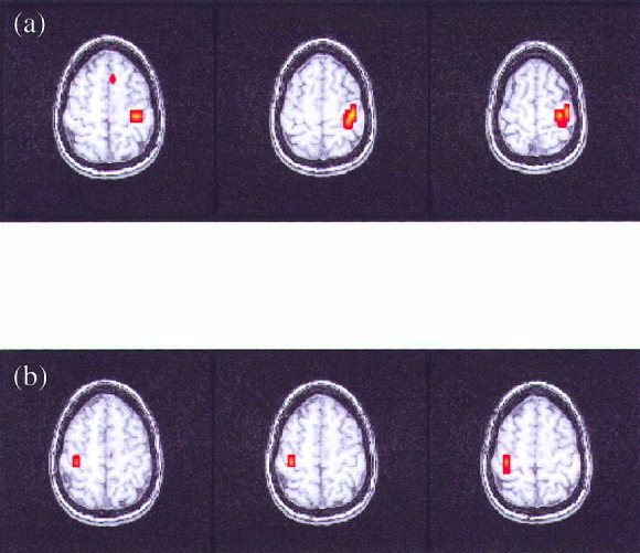
Functional maps of the analysis of the relative phases presented in three contiguous slices for the right‐hand (a) and left‐hand (b) finger‐tapping task.

Figure 4.

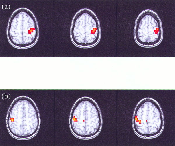
Functional maps presented in three contiguous slices for the right‐hand (a) and left‐hand (b) finger‐tapping task analyzed with SPM'99.

It was mentioned previously that an interrelation between instantaneous phases might occur in cases where the original time series may be unrelated. An example of this situation is shown in Figure 5 in which a time series from a voxel in the left motor cortex and the reference function for right‐hand tapping are plotted. The analysis of the relative phases revealed that the instantaneous phase of this time series was significantly related to the instantaneous phase of the reference function; however, correlation analysis revealed a coefficient of 0. 1113 when these two time series were compared. Traditional methodology would not have identified this voxel as being active during the task. In the five data sets analyzed, approximately 10% of the voxels determined to have a significant phase relationship with the reference time series were found to be phase‐locked but uncorrelated with the reference time series. All of these voxels were located in the primary motor cortex.

Figure 5.

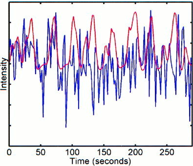
Time series and reference function that show a significant interrelation between instantaneous phases, but are not strongly correlated.

DISCUSSION

Analysis of the instantaneous phase signals of the time series in fMRI via the Hilbert transform was used as a method of determining the occurrence of an interrelation between phases. By applying the theory of phase synchronization to motor task data, we have determined that it is possible to detect these dependencies in the primary motor cortex during a randomized motor task. The functional maps created closely resemble typical fMRI motor activation maps. Results of the surrogate data testing have shown us that there is some feature of the data that is responsible for the instantaneous phase relationship that we have detected between the reference function and a small number of voxel time series. It remains to be determined if there is a physiological significance to the results presented in this study.

We investigated the relationship between instantaneous phases as a method of detecting activation by determining if the phase locking condition was fulfilled using the time series of the voxels and the reference function of the task performed, as opposed to investigating the synchronization occurring between two voxels. As we did not wish to use the data itself as part of the processing and rely on a priori anatomical information, we subsequently chose to incorporate the use of the reference function into the method. The reference function is not an oscillator that generates its own rhythms, and so it is not a self‐sustained oscillator. Thus, we are not truly characterizing phase synchronization in fMRI activation data, but are instead detecting the presence of a relationship between the instantaneous phases of the voxel time series and the reference function. Further investigation is in progress to determine a method for truly characterizing phase synchronization in fMRI time series. This future work is relevant to the issues raised in several studies concerning the linearity of fMRI data [Berns et al., 1999; Kershaw et al., 2001; Vasquez and Noll, 1998]. If we assume that there is an interesting source of nonlinearity present in fMRI data, we are left with the question of how to account for nonlinear interactions between regions of the brain. Linear correlations do not correctly characterize dependencies in multivariate time series data with strong nonlinear sources [Kantz and Schreiber, 1997]. Investigating the occurrence of phase synchronization between two voxel time courses will provide a method of detecting interactions between subsystems in nonlinear data.

In this method we have analyzed experimentally obtained time series data to detect the occurrence of phase locking. A criticism of this method might be that because these time series are bounded, this implies that the phase difference signals are also bounded, and perhaps the analysis should reveal that all the signals are always phase locked. This is a valid argument; however, it is important to remember that we are not just detecting the presence of the phase locking, but have computed a synchronization index and applied a method of statistical inference to test the significance of our results.

There has been some debate concerning the stationarity of fMRI data. The General Linear Model assumes that fMRI time series are stationary [Friston et al., 1995], but there have been studies that suggest otherwise [Berns et al., 1999; Calhoun et al., 1999; Gaschler‐Markefski et al., 1997]. It is important to note that the Hilbert transform does not require the time domain signals to be stationary [Rosenblum et al., 1997; Schafer et al., 1999]. While investigating the relationship between phases in nonstationary data, the analysis presented here should be completed by processing the signals with a sliding window approach. We chose to proceed with the assumption that fMRI data is stationary; however, this issue does warrant further consideration.

This method relies on the analysis of the phases of signals, whereas traditional methods rely on analysis of the signals themselves. We have shown that by examining the instantaneous phases to detect fMRI activation, relationships between the phases of two or more signals may be detected whereas the signals themselves may reveal no interdependence. We conclude that the analysis of the relative phases can be used in fMRI as a method of detecting a relationship between the reference function and voxels that are active during a motor task. We have verified this method on human subjects during an event‐related motor task study, and have discussed its implementations on nonstationary data. The method presented here offers a unique interpretation of an fMRI data set, allowing us to gain new insights into the complex behavior of the fMRI time series.

REFERENCES

- Aguirre GK, Zarahn E, D'Esposito M (1997): Empirical analyses of BOLD fMRI statistics II. Spatially smoothed data collected under null‐hypothesis and experimental conditions. Neuroimage 5: 199–212. [DOI] [PubMed] [Google Scholar]
- Aschoff J, Daan S, Groos GA (1982): Vertebrate circadian systems: structure and physiology. New York: Springer‐Verlag. [Google Scholar]
- Bendat JS, Piersol AG (2000): Random data analysis and measurement procedures. New York: John Wiley & Sons. [Google Scholar]
- Berns GS, Song AW, Mao H (1999): Nonlinear spatiotemporal dynamics of functional MRI revealed by independent components analysis. In: Proceedings of the First Joint BMES/EMBS Conference. 2:1184.
- Blekhman II (1988): Synchronization in science and technology. New York: ASME Press. [Google Scholar]
- Bramble DM, Carrier DR (1983): Running and breathing in mammals. Science 219: 251–256. [DOI] [PubMed] [Google Scholar]
- Bullmore E, Long C, Suckling J, Fadili J, Calvert G, Zelaya F, Carpenter AC, Brammer M (2001): Colored noise and computational inference in neurophysiological (fMRI) time series analysis: resampling methods in time and wavelet domains. Hum Brain Mapp 12: 61–78. [DOI] [PMC free article] [PubMed] [Google Scholar]
- Calhoun V, Adali T, Pearlson G (1999): (Non)stationarity of temporal dynamics in FMRI. In: Proceedings of the First Joint BMES/EMBS Conference. 2:1079.
- Edgington ES (1995): Randomization tests. New York: Marcel Dekker. [Google Scholar]
- Flandrin P (1992): Wavelet analysis and synthesis of fractional Brownian motion. IEEE Trans Info Theory 38: 910–917. [Google Scholar]
- Friston KJ, Holmes AJ, Worsley KJ, Poline J‐P, Frith CD, Frackowiak RSJ (1995): Statistical parametric maps in functional imaging: a general linear approach. Hum Brain Mapp 2: 189–210. [Google Scholar]
- Gabor D (1946): Theory of communication. J IEE London 93: 429–457. [Google Scholar]
- Gaschler‐Markefski B, Baumgart F, Tempelmann C, Schindler F, Stiller D, Heinze H‐J, Scheich H (1997): Statistical methods in functional magnetic resonance imaging with respect to nonstationary time‐series: auditory cortex activity. Magn Reson Med 38: 811–820. [DOI] [PubMed] [Google Scholar]
- Gray C, Singer W (1989): Stimulus‐specific neuronal oscillations in orientation columns of cat visual cortex. Proc Natl Acad Sci USA 86: 1698–1702. [DOI] [PMC free article] [PubMed] [Google Scholar]
- Hayashi C (1964): Nonlinear oscillations in physical systems. New York: McGraw‐Hill. [Google Scholar]
- Holmes AP, Blair RC, Watson JDG, Ford I (1996): Nonparametric analysis of statistic images from functional mapping experiments. J Cereb Blood Flow Metab 16: 7–22. [DOI] [PubMed] [Google Scholar]
- Kantz H, Schreiber T (1997): Nonlinear time series analysis. Cambridge, UK: Cambridge University Press. [Google Scholar]
- Kershaw J, Kashikura K, Zhang X, Abe S, Kanno I (2001): Bayesian technique for investigating linearity in event‐related BOLD fMRI. Magn Reson Med 45: 1081–1094. [DOI] [PubMed] [Google Scholar]
- Lachaux J‐P, Rodriguez E, Martinerie J, Varela FJ (1999): Measuring phase synchrony in brain signals. Hum Brain Mapp 8: 194–208. [DOI] [PMC free article] [PubMed] [Google Scholar]
- Makarenko V, Llinas R (1998): ); Experimentally determined chaotic phase synchronization in a neuronal system. Proc Natl Acad Sci USA 95: 15747–15752. [DOI] [PMC free article] [PubMed] [Google Scholar]
- Mandelbrot BB, Van Ness JW (1968): Fractional Brownian motions, fractional noises and applications. SIAM Rev 10: 422–437. [Google Scholar]
- Minorsky N (1974): Nonlinear oscillations. Huntington, New York: Robert E. Krieger Publishing Company. [Google Scholar]
- Neiman A, Pei X, Russell D, Wojtenek W, Wilkens L, Moss F, Braun HA, Huber MT, Voigt K (1999): Synchronization of the noisy electrosensitive cells in the paddlefish. Phys Rev Lett 82: 660–663. [Google Scholar]
- Nichols TE, Holmes AP (2002): Nonparametric permutation tests for functional neuroimaging: a primer with examples. Hum Brain Mapp 15: 1–25. [DOI] [PMC free article] [PubMed] [Google Scholar]
- Palus M, Hoyer D (1998): Detecting nonlinearity and phase synchronization with surrogate data. IEEE Eng Med Bio Mag 17: 40–45. [DOI] [PubMed] [Google Scholar]
- Percival DB (1999): Wavelet‐based surrogates for testing time series. In: Proceedings of the First Joint BMES/EMBS Conference. 1:910.
- Pikovsky A, Rosenblum M, Kurths J (2000): Phase synchronization in regular and chaotic systems: a tutorial. Int J Bifurcat Chaos 10: 2291–2306. [Google Scholar]
- Prichard D, Theiler J (1994): Generating surrogate data for time series with several simultaneously measured variables. Phys Rev Lett 73: 951–954. [DOI] [PubMed] [Google Scholar]
- Rosenblum MG, Pikovsky AS, Kurths J (1996): Phase synchronization of chaotic oscillators. Phys Rev Lett 76: 1804–1807. [DOI] [PubMed] [Google Scholar]
- Rosenblum MG, Pikovsky AS, Kurths J (1997): Phase synchronization in driven and coupled chaotic oscillators. IEEE Trans Circuits Syst 44: 874–881. [Google Scholar]
- Rosenblum MG, Kurths J, Pikovsky A, Schafer C, Tass P, Abel H‐H (1998): Synchronization in noisy systems and cardiorespiratory interaction. IEEE Eng Med Bio Mag 17: 46–53. [DOI] [PubMed] [Google Scholar]
- Saad ZS, Ropella KM, Cox RW, DeYoe EA (2001): Analysis and use of FMRI response delays. Hum Brain Mapp 13: 74–93. [DOI] [PMC free article] [PubMed] [Google Scholar]
- Schafer C, Rosenblum MG, Abel H‐H, Kurths J (1999): Synchronization in the human cardiorespiratory system. Phys Rev E 60: 857–870. [DOI] [PubMed] [Google Scholar]
- Schreiber T, Schmitz A (2000): Surrogate time series. Physica D 142: 346–382. [Google Scholar]
- Shannon CE, Weaver W (1949): The mathematical theory of communication. Urbana, Illinois: The University of Illinois Press. [Google Scholar]
- Stratonovich R (1963): Topics in the theory of random noise. New York: Gordon and Breach. [Google Scholar]
- Tass P, Rosenblum MG, Weule J, Kurths J, Pikovsky A, Volkmann J, Schnitzler A, Freund H‐J (1998): Detection of n:m phase locking from noisy data: application to magnetoencephalography. Phys Rev Lett 81: 3291–3294. [Google Scholar]
- Tewfik AH, Kim M (1992): Correlation structure of the discrete wavelet coefficients of fractional Brownian motion. IEEE Trans Info Theory 38: 904–909. [Google Scholar]
- Toronov V, Franceschini MA, Filaci M, Fantini S, Wolf M, Michalos A, Gratton E (2000): Near‐infrared study of fluctuations in cerebral hemodynamic during rest and motor stimulation: temporal analysis and spatial mapping. Med Phys 27: 801–815. [DOI] [PubMed] [Google Scholar]
- Vazquez AL, Noll DC (1998): Nonlinear aspects of the BOLD response in functional MRI. Neuroimage 7: 108–118. [DOI] [PubMed] [Google Scholar]
- Zarahn E, Aguirre GK, D'Esposito M (1997): Empirical analyses of BOLD fMRI statistics I. Spatially unsmoothed data collected under null‐hypothesis conditions. Neuroimage 5: 179–197. [DOI] [PubMed] [Google Scholar]