DeepHarmony: A deep learning approach to contrast harmonization across scanner changes

Abstract

Magnetic resonance imaging (MRI) is a flexible medical imaging modality that often lacks reproducibility between protocols and scanners. It has been shown that even when care is taken to standardize acquisitions, any changes in hardware, software, or protocol design can lead to differences in quantitative results. This greatly impacts the quantitative utility of MRI in multi-site or long-term studies, where consistency is often valued over image quality. We propose a method of contrast harmonization, called Deep-Harmony, which uses a U-Net-based deep learning architecture to produce images with consistent contrast. To provide training data, a small overlap cohort (n=8) was scanned using two different protocols. Images harmonized with DeepHarmony showed significant improvement in consistency of volume quantification between scanning protocols. A longitudinal MRI dataset of patients with multiple sclerosis was also used to evaluate the effect of a protocol change on atrophy calculations in a clinical research setting. The results show that atrophy calculations were substantially and significantly affected by protocol change, whereas such changes have a less significant effect and substantially reduced overall difference when using DeepHarmony. This establishes that DeepHarmony can be used with an overlap cohort to reduce inconsistencies in segmentation caused by changes in scanner protocol, allowing for modernization of hardware and protocol design in long-term studies without invalidating previously acquired data.

1. Introduction

Magnetic resonance imaging (MRI) is a non-invasive, tunable medical imaging technique commonly used to detect differences in the soft tissue of the body, especially in the brain. However, the flexibility that is inherent in MRI often comes with drawbacks in terms of reproducibility. First, a lack of quantitative standardization between scanners leads to inter-scanner variability, even for data acquired by scanners of the same manufacturer [1].

Second, differences in scan protocol design lead to variation in the appearance of a specific image type (or contrast) between different studies. For example, a T1-weighted image may be treated similarly by an analysis algorithm or a reviewer, but can be acquired in many ways. In addition, a change in scan acquisition can lead to associated differences in quantitative results [2, 3, 4, 5], diluting effects that a researcher may want to investigate and limiting the utility of MRI in clinical applications such as precision medicine. These issues can cause a lag in the imaging technology that is employed—especially in large-scale, multi-site, or longitudinal studies— where consistency in scanning outweighs advances that might be available. Contrast harmonization promises to be a powerful aid in overcoming these problems by providing quantitatively and qualitatively consistent images for automated algorithms and manual reviewers.

Many methods have been proposed to correct differences in contrast between scans, including statistical modeling of quantitative results [6, 7, 8] and global alterations of the image histogram [9, 10, 11, 12]. However, statistical models require a method of analysis (i.e., segmentation) to produce a feasible result before correction can take place. This can mean that modern machine learning algorithms, such as deep learning-based methodologies, cannot be corrected, as the output may be nonsensical if the testing data differs too much from the training data. Histogram models (linear [12] and piecewise [10]) can also be problematic as they do not use local contrast information and instead assume global histogram correspondence between images. This assumption can break down in many cases including subjects with pathological differences, where global biological changes can change the proportions in the global histogram, even without any change in contrast. Recently, example-based synthesis has also been proposed as a method for contrast harmonization [13, 14]. More recent work has also explored the realm of deep learning-based synthesis, specifically using adversarial frameworks [15, 16, 17, 18]. While synthesis techniques are traditionally used for creation of a contrast not in the input set, they can also be repurposed to create a harmonized version of an input contrast. However, in this framework, there is an important distinction between harmonization and traditional synthesis. While each applies similar techniques, the goals are distinct. In traditional synthesis, the goal is to accurately recreate a missing contrast or modality, whereas in harmonization the goal is to create two similar contrasts that can be compared quantitatively. Nevertheless, synthesis techniques can be easily used to create an appropriate contrast and can act as a starting point to produce a harmonization framework.

In this work, we present DeepHarmony, a deep fully-convolutional neural network (DFCNN) based on the U-Net architecture [19, 20] for contrast harmonization using a small overlap cohort as training data. By incorporating multi-contrast information to produce multiple output contrasts from a combined network set, DeepHarmony outperforms other comparable methods in direct comparison using the overlap cohort and demonstrates quantitatively consistent results in a similarly acquired long-term longitudinal cohort. A preliminary version of DeepHarmony appeared in a conference paper by Dewey et al. [21]

2. Materials and Methods

Our proposed method used a small overlap cohort acquired in two scanning environments: Protocol #1 and Protocol #2 (described in Table 1). These data were used to train a DFCNN, which was used to harmonize images between the different protocols. We validated our methodology in the overlap cohort against results from competing methodologies and the acquired, preprocessed images, then applied this method for additional validation purposes in a longitudinal clinical cohort.

Table 1:

Scanner and protocol specifications

	Protocol #1	Protocol #2
Scanner Hardware	Philips Achieva 3T	Philips Achieva 3T
Scanner Software	R3.2.3	R5.1.7
Receive Coil	16ch Neurovascular	32ch Head
T1-weighted	MPRAGE	MEMPRAGE
	1.1 × 1.1 × 1.18mm*	1 × 1 × 1mm
	TE=6ms, TR=3s, TI=840ms	TE=6.2ms, TR=2.5s, TI=900ms
FLAIR	2D TSE	3D VISTA (TSE)
	0.83 × 0.83 × 2.2mm†	1 × 1 × 1mm
	TE=68ms, TR=11s, TI=2.8s	TE=125ms, TR=4.8s, TI=1.6s
PD-/T2-weighted	2D TSE	2D TSE
	1.1 × 1.1 × 2.2mm*	1 × 1 × 3mm
	TE=12ms/80ms, TR=4.2s	TE=11ms/100ms, TR=3.4s

^*Scan is reconstructed on the scanner 0.83x0.83mm in-plane by zero-padding in frequency space.

^†A small subset of FLAIR images (n=18) in the longitudinal cohort were acquired with 4.4mm slices.

2.1. Data

To create a training dataset for all harmonization methods, 12 subjects (10 subjects with multiple sclerosis (MS) and 2 healthy subjects) were scanned twice within 30 days on two separate Philips Achieva 3T scanners (Philips Healthcare, Best, The Netherlands) with differing hardware and a different scanning protocol according to the scan parameters in Table 1. Each scan included a set of standard structural images with a 3D T1-weighted image, a 2D or 3D T2-FLAIR image and a 2D dual-echo PD-/T2-weighted image. Additionally, longitudinal data were retrospectively collected from 45 patients with relapsing remitting MS over 10 years as a part of a long-term MRI study. Most of the longitudinal cohort comprised of scans acquired with Protocol #1 and each subject was required to have at least two scans with at least one scan collected using Protocol #2. Data acquired using Protocol #2 was, as of yet, unused for clinical research due to differences in initial results.

2.2. Preprocessing

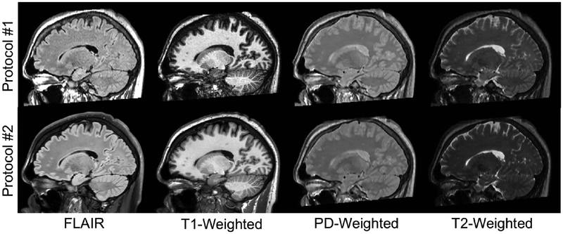
All images were converted to the Neuroimaging Informatics Technology Initiative (NIfTI-1) file format (http://nifti.nimh.nih.gov) and reoriented to a common axial orientation. Images were corrected for inhomogeneity using N4BiasFieldCorrection [22] and all 2D acquired images were super-resolved and anti-aliased using Synthetic Multi Orientation Resolution Enhancement (SMORE) [23]. All contrasts for subjects in the overlap cohort were then rigidly registered to the T1-weighted image from Protocol #2. Each registration involved three registration steps implemented using the Advanced Normalization Tools (ANTs) software package [24]. First, multiple initial registration conditions are attempted to avoid local minima, then images are rigidly registered using the entire image, and finally images are rigidly registered again only utilizing brain voxels isolated with ROBEX [25]. After registration, all images were gain-corrected by linearly adjusting the intensities to align the white matter histogram peaks (WMPs). The WMP was determined by calculating the mean intensity of a rough white matter mask, where rough tissue masks were calculated on the T1-weighted images using fuzzy C-means within the ROBEX mask to isolate regions of white matter, grey matter, and cerebrospinal fluid [26]. Gain-corrected, co-registered images were then used as inputs for harmonization and as a comparison for harmonized results. Examples of preprocessed images in the sagittal orientation for one subject in the overlap cohort are shown in Figure 1.

Figure 1:

Preprocessed images from one subject from the overlap cohort depicting the four input (Protocol #1) and four target (Protocol #2) contrasts.

2.3. Harmonization

2.3.1. U-Net Implementation

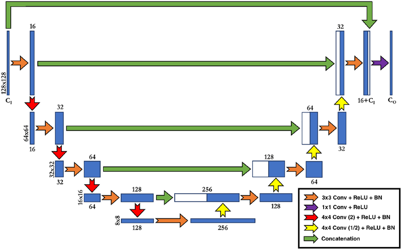
The neural network implemented for DeepHarmony was modeled after the U-Net architecture, which has been shown to perform well in tasks of medical image segmentation and synthesis [27, 20]. In order to optimize the network for harmonization, the network used here contains a number of important differences from the vanilla U-Net implementation (see Figure 2). The first of these differences is the addition of a final concatenation step (introduced by Zhao et al. [20]) between the input contrasts and the final feature map (the green arrow across the top of Figure 2). This allows the network to include the input contrasts in the final 1x1 convolutional layer, directing the final feature maps to only augment the input contrasts, instead of recreating the target contrasts entirely. The second difference in design is the introduction of strided convolution (and deconvolution) as the method for downsampling (and upsampling) the feature maps. This methodology replaces the maximum pooling (and nearest neighbor upsampling) and convolution steps that are present in Zhao et al. [20]. This allows for a network with only convolution blocks, which we have empirically observed to have improved performance. Traditionally, strided convolution and deconvolution are avoided due to hashing artifacts that are common [28], but a combination of 4×4 kernels and suffcient training eliminates the need for alternate methods in this design. Finally, the number of parameters in the network was significantly reduced (~ 4× from Ronneburger et al. [19] and ~ 2× from Zhao et al. [20]) to produce a lighter weight network, which is quicker to train. The network was implemented in SynMI¹ using the Keras API library [29] and the Tensorflow backend [30].

Figure 2:

Diagram of DeepHarmony U-Net Implementation. Convolutions with (2) or (1/2) indicate strided convolutions with stride of 2 or 1/2, respectively. C_I and C_O refer to the number of input and output contrasts, respectively. All convolutions are followed by a rectified linear unit (ReLU) and batch normalization (BN), except the final 1×1convolution, which does not use normalization.

2.3.2. Network Training

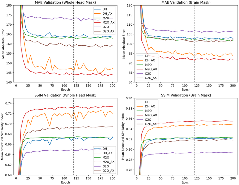
To provide adequate training, validation, and testing data, 6-fold cross-validation was performed at the subject level using a 8/2/2 split for training, validation, and testing, respectively. In this way, each image was used for validation and testing by using a trained network that had not yet seen the subject. This methodology is in contrast to a full leave-one-out validation, as we found empirically that 8 subjects was sufficient for training. This allowed for improved computation time as only half as many training rounds were required. For training, 128 × 128 patches were built from the input and target images centered around each non-zero voxel. These patches were then randomly selected with replacement to create a training batch. Training of each network was carried out on a NVIDIA K80 GPU for 200 epochs using a batch size of 8 and 250 batches per epoch. Mean absolute error (MAE) was used as the training loss function to allow for small differences to contribute more than would be possible when using mean squared error. Adam [31] was used as the optimizer with a learning rate of 0.001. No regularization or dropout was used in training. Training time for 200 epochs was approximately 160 minutes. Validation was performed post-hoc after training had been completed by saving the network weights every 5 epochs. Mean Structured Similarity Index (SSIM) and MAE (averaged over all four contrasts) were used as validation metrics over 6 folds of size 2 to determine a proper stopping point for training. Validation metrics were also calculated over a whole-head mask and a brain mask determined on the input images allowing for comparison of how the network was performing both within the brain area and on the head as a whole.

2.3.3. Multi-Contrast Training

In MRI, each of the contrasts (or pulse sequences) in a scanning session provides a mix of complementary and overlapping information. For this reason, Deep Harmony was developed for multi-contrast inputs and outputs. By using all input contrasts to predict all output contrasts simultaneously, the network can use any piece of each of the input contrasts when predicting the required outputs. This also has the benefit of a factor of four decrease in training time, as only one network is required to harmonize all of the inputs. For this study, Deep Harmony was compared to two other training variants: one-to-one (O2O) and many-to-one (M2O). Both variants use the implement the same general architecture as DeepHarmony. The O2O variant takes a single contrast from the Protocol #1 scan and produces the corresponding contrast from the Protocol #2 scan. For this method, four separate networks must be trained, one for each of the contrast pairs. The M2O method differs from O2O in that it uses all four of the input contrasts (T1-weighted, FLAIR, PD-weighted, and T2-weighted) from Protocol #1 to predict a single output contrast from Protocol #2. This method also requires four networks to be trained, but each one will take in all of the complementary contrast information, resulting in only about 500 additional parameters compared to the O2O network.

2.3.4. 2.5D Inference

As can be seen in Figure 2, the DeepHarmony architecture is designed for 2D images. This is in contrasts to modern MRI scans which are 3D volumes. Although fully 3D deep networks are possible (and may be considered in future work), we observed that harmonization works very well with the use of the much faster 2D networks, which also allow for a larger training data pool since each image slice is unique. On the other hand, three natural orientations—axial, sagittal, and coronal—are available for use. So, to exploit these three orientations and to provide additional robustness to artifacts or other variations that may exist in the data, DeepHarmony uses three separately trained networks to predict the final volumes. Each of these networks is trained on patches extracted from one of the three orthogonal orientations. Then, during prediction, the input patches are extracted in the same three orientations and fed into the appropriate network. This produces three directional volumes, which are combined using a voxel-wise median to produce a final volume. In this study, the axial network results for each of the training methods described in Section 2.3.3 (O2O AX, M2O AX, and DH AX) were also compared.

2.3.5. Harmonizing Protocol #2

Images that are generated using a harmonization process demonstrate noise characteristics that are indicative of a synthetic image; in particular, they are generally less noisy. In addition, it has been demonstrated previously that the addition of a “self-synthesis” step in the target image domain greatly improves the consistency of synthesized images between domains without affecting the contrast of the target image [32]. Therefore, in order to create fully harmonized images, Deep Harmony forces all images to be passed through a harmonization process. This ensures that each image shares the same noise characteristics regardless of which protocol the images were acquired with. To facilitate this, a separate secondary harmonization network is trained using the Protocol #2 images as input and an identical network structure as the forward path. Traditionally, the same images would be used as outputs, however, as deep networks can easily produce an identity transform, the harmonized Protocol #1 images are used as targets for the secondary network to encourage the network to generate synthetic-looking images.

2.3.6. Competing Methods

Two additional methods were tested on the overlap cohort to establish the current state-of-the-art: a deep learning-based fused latent space method (MMBS) by Chartsias et al. [33], and a random forest-based method inspired by Jog et al. (REPLICA) [13, 26]. Each of these methods was trained according to published methods using the M2O approach, where all input contrasts were used as inputs and a single contrast was predicted. The published MMBS code was rewritten to use TensorFlow instead of Theano to reduce software dependency issues that caused errors in the published code. To compare MMBS and REPLICA results directly with the Deep Harmony results, a secondary harmonization model was created using each of these two methods as well. Comparison of all methods (including the acquired images) was performed using MAE and SSIM over a whole-head mask and a brain mask.

2.4. Segmentation

Segmentation of all scans followed the same processing pipeline. First, skull removal and intracranial volume (ICV) estimation were performed using MONSTR [34]. MONSTR uses both the T1-weighted and T2-weighted images to provide an accurate estimation of the inner surface of the skull and therefore correctly accounts for CSF outside of the brain. After skull removal, images were segmented using an established pipeline [35] consisting of lesion segmentation (if lesions were present) [36], lesion filling using the lesion filling tool in the FSL software package [37], and whole-brain segmentation and cortical surface estimation using Joint Label Fusion (JLF) [38] and MACRUISE [39]. Volumes were compared using Dice similarity coefficient (DSC), percent volume difference (PVD), and volume bias (signed volume difference). Statistical testing for image and volume comparison were conducted in a paired fashion using the Wilcoxon signed-rank test with α = 0.05 (correcting for multiple comparisons using Bonferroni Correction). Results stated as “significant” are statistically significant with respect to this testing.

2.5. Longitudinal Analysis

In the longitudinal cohort, all preprocessing was performed identically to the overlap cohort with the addition of a longitudinal registration component to the image from the baseline time point. A DeepHarmony model was trained using all 12 overlap subjects to provide the best generalization, as the overlap and longitudinal cohorts were mutually exclusive. Acquired and harmonized images were segmented using the same procedures as outlined in Section 2.4 and each volume was calculated as a percentage of the baseline ICV to normalize for head size. To evaluate the harmonized results, the following linear mixed effects model

$$v_{i,j}={\beta }_0+{\beta }_1\cdot f_{i,j}+{\beta }_2\cdot a_i+{\beta }_3\cdot s_i+{\beta }_4\cdot f_{i,j}\cdot a_i+{\beta }_5\cdot f_{i,j}\cdot s_i+{\beta }_6\cdot p_{i,j}+{ϵ}_i$$ (1)

was used to predict substructure volumes v, for a subject i at scan time point j, from clinical fixed effects with subject as a random effect [40]. Here, follow-up f was measured from baseline in years, sex s was coded as 0 for male and 1 for female, protocol p was coded as 0 for Protocol #1 and 1 for Protocol #2, age a was measured at baseline in years and centered at 45 years.

The interaction between protocol and follow-up was not investigated in this study due to the limited follow-ups that were acquired using Protocol #2. A random subject intercept ϵ_i was included to account for random variation between subjects. To determine the effect of protocol on the model, β₆ was extracted from the model and evaluated for significance using Welch’s t-test for unequal variances.

3. Results

3.1. Training Validation

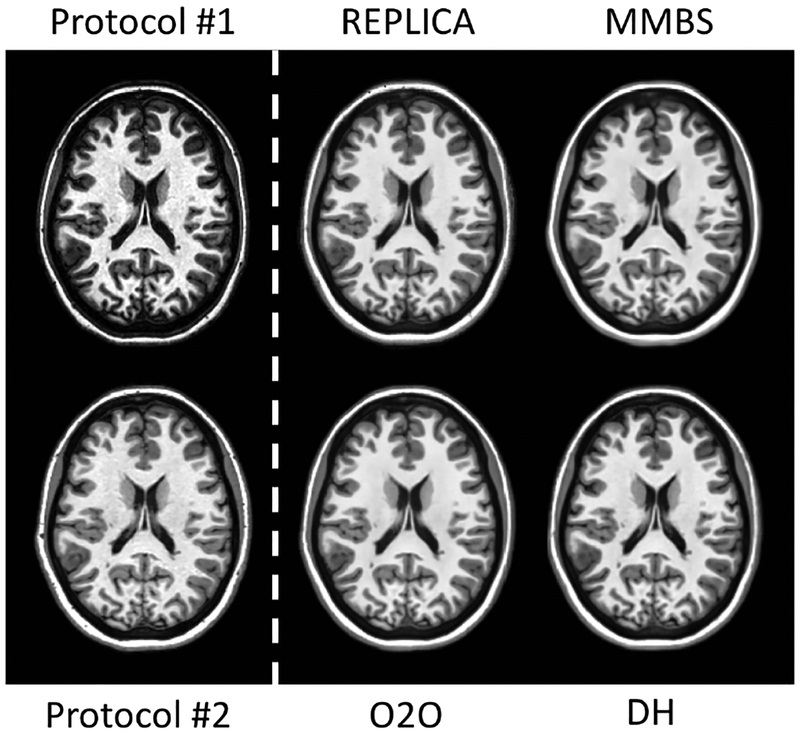
Validation of the DeepHarmony networks was performed post-hoc using MAE and SSIM on both a whole-head mask and a brain mask. Figure 3 depicts metrics calculated on the validation data as the training progressed. Specifically, the figure shows MAE and SSIM calculated over each of the brain and head masks to determine the effect of harmonization inside the brain and over the whole head. Initially, early stopping was investigated to determine the proper training length; however, this stopping point differed for each metric, so no single epoch could be singled out as the best perform ing. Because of this, models at 120 epochs were chosen empirically, as all metrics were within a small difference from their respective minimum (or maximum) values. The same number of epochs was used for the secondary Protocol #2 networks for consistency. MMBS was trained with early stopping during the training process (as published [33]), thus no external validation was performed. Qualitative harmonization results from the validation set are shown in Figure 4, demonstrating very similar images from all harmonization methods.

Figure 3:

Validation graphs for deep network training. Dotted line represents chosen epoch for testing.

Figure 4:

Harmonized Protocol #1 T1-weighted images using REPLICA, MMBS, O2O, and DeepHarmony (DH). For comparison, the input contrast (Protocol #1) and the target contrast (Protocol #2) are displayed on the left side of the white, dashed line.

3.2. Image Similarity

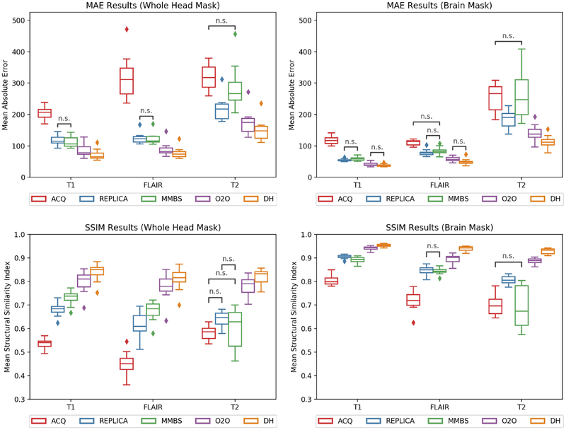
After completion of training, the reserved testing images were harmonized with the appropriate network and both volumes and comparison metrics were calculated. The acquired images (ACQ), including preprocessing with super-resolution and anti-aliasing, were also used for comparison. Image similarity was compared using MAE and SSIM for each contrast, and selected results

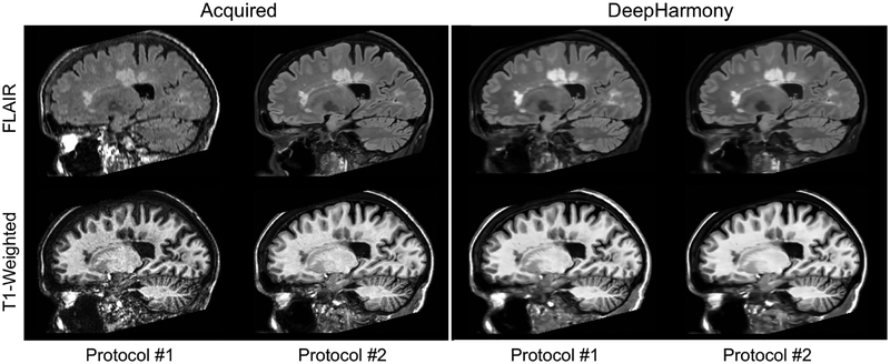
are shown graphically in Figure 5. Additionally, peak signal-to-noise ratio (PSNR) was calculated between the overlap images, but these results are not shown because they are highly correlated with the MAE results. After harmonization, the 2.5D M2O method showed no significant difference from Deep Harmony for all metrics. Furthermore, the axial-only experiments performed significantly worse compared to their 2.5D counterparts for all metrics (e.g., O2O vs. O2O AX). Pairwise comparisons were generally statistically significant, except where marked with “n.s.” in Figure 5. An example showing the acquired images and results of harmonization with DeepHarmony (for T1-weighted and FLAIR images) are shown in Figure 6 for qualitative comparison. It is important to note that while there is extensive qualitative similarity of the harmonized versions of Protocol #1 and Protocol #2 images, these images do not completely match the appearance of the acquired image due to a reduction in image noise during the harmonization process. This is a hallmark of supervised synthesis with metrics such as MAE and does not affect the results of segmentation as seen below.

Figure 5:

Comparison of SSIM and MAE for T1-weighted, FLAIR, and T2-weighted contrasts over both whole head and brain masks. All pairwise comparisons are significant unless marked with “n.s.”.

Figure 6:

Representative sagittal slices for the same subject showing acquired images on the left and harmonized (using DeepHarmony) on the right.

3.3. Volumetric Similarity

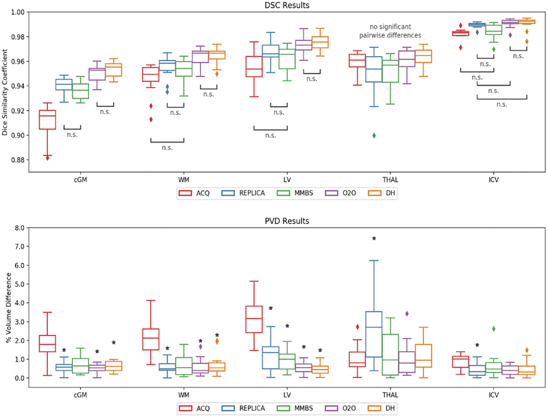
Volumes calculated from automatic segmentations were compared on four substructures of the brain (cortical gray matter: cGM, cerebral white matter; WM, lateral ventricles: LV, thalamus: THAL) and the intracranial volume (ICV). Results for DSC and PVD are presented graphically in Figure 7. For DSC, all pairwise comparisons were generally significant, except the thalamus segmentations which had no significant differences. For PVD, most comparisons were generally not significant with the exception of most comparisons to the ACQ results.

Figure 7:

DSC and PVD between segmented volumes using data from Protocol #1 and Protocol #2. In the top plot, all pairwise comparisons are significant except when marked with “n.s.”. In the bottom plot, the only significant differences are between ACQ and the methods marked with a star.

For all patients with white matter lesions (WML), volumes of segmented lesions also were compared. In this comparison, DeepHarmony showed significant improvement in both DSC and PVD over other methods (except O2O, where no significant difference was shown). O2O also showed a significant improvement over REPLICA. All other comparisons were not statistically significant.

In addition to absolute PVD, volume bias (signed volume difference) was evaluated to determine if volumes calculated were significantly larger or smaller on Protocol #2 than on Protocol #1. These results are presented in Table 2. DeepHarmony and O2O show a non-significant bias in all measured volumes, with DeepHarmony showing the smallest overall bias in multiple areas, with substantially decreased variance.

Table 2:

Mean volume bias (in %) from Protocol #1 to Protocol #2 in the overlap cohort after different normalization pipelines. Standard deviation over all subjects is also presented. Positive values indicate an increase in volume from Protocol #1 to Protocol #2. Bold values indicate the bias is significant when compared to 0.

	ACQ	REPLICA	MMBS	O2O	DeepHarmony
Cortical GM	1.84 ± 0.82	0.23 ± 0.62	0.30 ± 0.78	0.26 ± 0.50	−0.05 ± 0.26
Cerebral WM	−2.17 ± 0.95	−0.34 ± 0.60	−0.55 ± 0.72	0.23 ± 0.69	0.35 ± 0.88
Thalamus	0.94 ± 0.87	2.72 ± 1.79	0.54 ± 1.62	0.21 ± 1.42	−0.27 ± 1.37
Lateral Ventricles	−3.24 ± 1.06	−1.19 ± 0.79	−0.50 ± 0.99	−0.30 ± 0.58	0.10 ± 0.55
ICV	−0.75 ± 0.59	−0.38 ± 0.40	−0.21 ± 0.92	0.16 ± 0.47	0.18 ± 0.49
WML	30.49 ± 39.28	49.69 ± 54.76	9.57 ± 56.03	−12.87 ± 34.40	−1.89 ± 19.53

Finally, to verify that the harmonized images produced volumes consistent with the target scanner (Protocol #2), volumes from harmonized images (both Protocol #1 and Protocol #2) were compared to the volumes obtained directly from the acquired Protocol #2 images. Almost all differences were not significant except for the lateral ventricle volume using the O2O and the REPLICA methods.

3.4. Longitudinal Stability

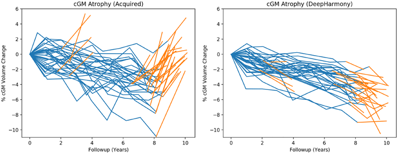
The benefits of harmonization can be seen in the plots of cGM atrophy in Figure 8. For the harmonized data, the atrophy measurements are not only stable over the change in protocol, but there is also a more consistent atrophy pattern in the group of subjects and in the individual patient trajectories. This is matched with stronger relationships between the modeled variables measured by R² and a substantially reduced overall variance. In Table 3, there is a substantial decrease in the intercept related to protocol (β₆ in Equation 1) when using harmonized images. In addition, only the cGM volume from harmonized data retained a significant effect of protocol on the model, whereas all volumes from the acquired data show a significant effect.

Figure 8:

Longitudinal trajectories for cortical grey matter (in % from baseline). Protocol #1 is shown in blue and Protocol #2 is shown in orange.

Table 3:

Scanner effect in longitudinal prediction of substructure volumes from clinical covariates. Bold values indicate a statistically significant effect.

	Acquired		DeepHarmony
	β6	p-value	β6	p-value
Cortical GM	5.08%	<0.0001	−0.64 %	0.02
Cerebral WM	3.56%	<0.0001	0.48%	0.08
Thalamus	2.32%	<0.001	0.20%	0.78
Lateral Ventricles	−6.89 %	<0.0001	0.23%	0.88

4. Discussion

We presented DeepHarmony, a method to harmonize datasets collected in the presence of scanner changes through the acquisition of an overlap cohort. Our method was able to accurately transform images from two different scanning protocols to produce harmonized versions that mimicked the contrast of the target protocol qualitatively and in volumetric analyses. In training, 2.5D reconstruction was found to stabilize the training process when compared to a single axial prediction. While this affected the accuracy of the initial prediction, this difference was small and not significant once the appropriate harmonization network was applied to the Protocol #2 images. The use of a single DeepHarmony model, where all four input contrasts are used to predict all four target contrasts simultaneously, significantly improved harmonization in almost all cases when compared to a traditional contrast-to-contrast harmonization (O2O). When compared to state-of-the-art methods (REPLICA and MMBS) and the acquired, preprocessed images (ACQ), DeepHarmony shows significantly improved harmonization in all measurements. A potential critique of this work is the use of supervised learning, which requires the prospective acquisition of an overlap cohort. Recently, many unsupervised methodologies [15, 16] have been proposed, which would eliminate this requirement, but were not evaluated in this study, where prospective data was available. We hope to explore this in future work.

When looking at volumetric results, both O2O and DeepHarmony show significant improvement in DSC over the compared methods and ACQ. However, O2O and DeepHarmony were not significantly different from one another. This is particularly important as not all studies will include multi contrast data. For PVD, we see that no harmonization methods show significant differences from one another, but most methods show significant improvement compared to ACQ. This indicates that any of these harmonization methods will improve volumetric similarity. It is a possible critique that this study does not include images acquired at different field strengths or from different vendors. While this is true, there are substantial differences in the method of acquisition, most evident in the T1-weighted and FLAIR imaging. In future work, we hope to expand this to a multi-vendor, multi-site experiment to explore real-world harmonization scenarios, which may allow for better discrimination between methodologies. WML volume, however, was particularly difficult to characterize well in any setting due to the small, spurious nature of the lesions themselves, causing high amounts of variance between and within specific protocols. This did not adversely affect the other structures segmented, as most of the whole-brain segmentation relies on T1-weighted images. T1-weighted images have less conspicuous lesions, which can be avoided with approximate lesion filling and registration based fusion, which was used in this study. In the WML, the results from O2O and DeepHarmony are not significantly different from each other, but only DeepHarmony showed a significant improvement over the acquired results, due to the high variance in the segmentations.

While PVD mainly showed improvements when compared to ACQ, volume bias showed more substantial difference between methods. Here, for example, results from REPLICA demonstrated that although most measurements were significantly smaller in magnitude, there was still remaining bias between the segmentation results. MMBS also showed significant bias in the WM segmentation while both O2O and DeepHarmony showed no significant bias and the smallest overall bias on average. DeepHarmony showed particularly impressive reduction in bias for the cGM and WML volumes, which were very evenly distributed around zero, coupled with significant reduction in absolute volume difference. This is expected, as the O2O method does not use the high resolution T1-weighted information (available in DeepHarmony) when predicting FLAIR images used in lesion segmentation.

When considering the secondary Protocol #2 network, there is the possibility that the use of harmonized images as targets would essentially allow the results to meet in the middle, rather than truly duplicating the Protocol #2 contrast. This raises some concerns, as the goal of this process is to also accurately duplicate the contrast of the target protocol. However, we show that DeepHarmony shows no significant differences in volume when compared to the results from the acquired images of Protocol #2. This indicates that DeepHarmony accurately represents the target contrasts, while O2O, which also performed well in volumetric similarity, had significantly different LV volumes when compared to Protocol #2 results. In the future, different methods for harmonization of the Protocol #2 images, including deep networks for denoising and encouraging channel mixing will be evaluated in order to generate the synthetic quality of the harmonized images, even when the same Protocol #2 are used as the target.

In the longitudinal cohort, the effect of harmonization is quite evident, demonstrating two important points. First, the effect of protocol change on longitudinal segmentation is substantially reduced and is no longer a significant factor in modeling atrophy for most volumes. This is vital to the proper analysis of these data, as using the acquired data would dilute the effects measured by these sensitive atrophy metrics. Secondly, the effect of harmonization is not just limited to transitions from one protocol to another. It can also be seen that older historical data, which were always acquired with Protocol #1 also show more consistency from scan to scan. The tighter grouping and reduced variance (as shown in the right graph of Figure 8), coupled with better correlation in modeling, indicates an increase in overall stability of the segmentation from time point to time point, which will allow for more confidence to be placed in atrophy measurements over time. The remaining significant effect in the cGM volumes after harmonization is still a concern for longitudinal analysis. This could be improved by augmenting the DeepHarmony methodology with improvements such as fully 3D networks, adversarial training (e.g., pix2pix [41], MedGAN [17]) or DenseNets [42], which have been shown to improve accuracy and perceptual quality in computer vision and medical imaging tasks.

5. Conclusions

This paper introduces DeepHarmony, a fully-convolutional neural network for contrast harmonization that uses a prospectively acquired overlap cohort of patients scanned with each of two protocols (before and after a scanner change). This method incorporates multi-contrast data and 2.5D training/prediction to produce qualitatively and quantitatively similar images between the two protocols. We also show that images harmonized with DeepHarmony have significantly improved volume correspondence compared to acquired images and results from other methods. While absolute volume difference was not always significantly different between methods, only DeepHarmony, showed complete removal of bias between segmented volumes in both protocols, along with significant reduction of absolute volume difference. In addition, DeepHarmony allows for a longitudinal atrophy model that demonstrates no statistical effect of protocol in most volumes and substantially improved stability in longitudinal segmentation. These results indicate that comparisons across protocols using DeepHarmony may be valid and can be conducted with the acquisition of a small overlap cohort, providing the ability to update or change a scanning protocol when necessary, without compromising valuable existing data.

References

- [1].Shinohara RT, Oh J, Nair G, Calabresi PA, Davatzikos C, Doshi J,Henry RG, Kim G, Linn KA, Papinutto N, Pelletier D, Pham DL,Reich DS, Rooney W, Roy S, Stern W, Tummala S, Yousuf F,Zhu A, Sicotte NL, Bakshi R, NAIMS Cooperative, Volumetric Analysis from a Harmonized Multisite Brain MRI Study of a Single Subject with Multiple Sclerosis., American Journal of Neuroradiology 38 (8) (2017) 1501–1509, doi: 10.3174/ajnr.A5254. [DOI] [PMC free article] [PubMed] [Google Scholar]
- [2].Clark KA, Woods RP, Rottenberg DA, Toga AW, Mazziotta JC, Impact of acquisition protocols and processing streams on tissue segmentation of T1 weighted MR images, NeuroImage 29 (1) (2006) 185–202, ISSN 1053–8119, doi: 10.1016/j.neuroimage.2005.07.035. [DOI] [PubMed] [Google Scholar]
- [3].Han X, Jovicich J, Salat D, van der Kouwe A, Quinn B, Czanner S,Busa E, Pacheco J, Albert M, Killiany R, Maguire P, Rosas D,Makris N, Dale A, Dickerson B, Fischl B, Reliability of MRI-derived measurements of human cerebral cortical thickness: The effects of field strength, scanner upgrade and manufacturer, NeuroImage 32 (1) (2006) 180–194, ISSN 1053–8119, doi: 10.1016/j.neuroimage.2006.02.051. [DOI] [PubMed] [Google Scholar]
- [4].Biberacher V, Schmidt P, Keshavan A, Boucard CC, Righart R,Smann P, Preibisch C, Frbel D, Aly L, Hemmer B, Zimmer C, Henry RG, Mhlau M, Intra- and interscanner variability of magnetic resonance imaging based volumetry in multiple sclerosis, NeuroImage 142 (2016) 188–197, ISSN 1053–8119, doi: 10.1016/j.neuroimage.2016.07.035. [DOI] [PubMed] [Google Scholar]
- [5].Schnack HG, van Haren NE, Brouwer RM, van Baal GCM,Picchioni M, Weisbrod M, Sauer H, Cannon TD, Huttunen M,Lepage C, Collins DL, Evans A, Murray RM, Kahn RS, Hulsho Pol HE, Mapping reliability in multicenter MRI: Voxel-based morphometry and cortical thickness, Human Brain Mapping 31 (12) (2010) 1967–1982, doi: 10.1002/hbm.20991. [DOI] [PMC free article] [PubMed] [Google Scholar]
- [6].Chua AS, Egorova S, Anderson MC, Polgar-Turcsanyi M, Chitnis T, Weiner HL, Guttmann CR, Bakshi R, Healy BC, Using multiple imputation to e ciently correct cerebral MRI whole brain lesion and atrophy data in patients with multiple sclerosis, NeuroImage 119 (2015) 81–88, ISSN 1053–8119, doi: 10.1016/j.neuroimage.2015.06.037. [DOI] [PubMed] [Google Scholar]
- [7].Jones BC, Nair G, Shea CD, Crainiceanu CM, Cortese IC, Reich DS, Quantification of multiple-sclerosis-related brain atrophy in two heterogeneous MRI datasets using mixed-e ects modeling, NeuroImage: Clinical 3 (2013) 171–179, ISSN 2213–1582, doi: 10.1016/j.nicl.2013.08.001. [DOI] [PMC free article] [PubMed] [Google Scholar]
- [8].Fortin J-P, Sweeney EM, Muschelli J, Crainiceanu CM, Shinohara RT, Removing inter-subject technical variability in magnetic resonance imaging studies, NeuroImage 132 (2016) 198–212, ISSN 1053–8119, doi: 10.1016/j.neuroimage.2016.02.036. [DOI] [PMC free article] [PubMed] [Google Scholar]
- [9].He Q, Shiee N, Reich DS, Calabresi PA, Pham DL, Intensity standardization of longitudinal images using 4D clustering, in: 2013 IEEE 10th International Symposium on Biomedical Imaging, ISSN 1945–7928, 1388–1391, doi: 10.1109/ISBI.2013.6556792, 2013. [DOI] [Google Scholar]
- [10].Nyúl LG, Udupa JK, On standardizing the MR image intensity scale, Magnetic Resonance in Medicine 42 (6) (1999) 1072–1081. [DOI] [PubMed] [Google Scholar]
- [11].Shah M, Xiao Y, Subbanna N, Francis S, Arnold DL, Collins DL,Arbel T, Evaluating intensity normalization on MRIs of human brain with multiple sclerosis, Medical Image Analysis 15 (2) (2011) 267–282, ISSN 1361–8415, doi: 10.1016/j.media.2010.12.003. [DOI] [PubMed] [Google Scholar]
- [12].Shinohara RT, Sweeney EM, Goldsmith J, Shiee N, Mateen FJ, Calabresi PA, Jarso S, Pham DL, Reich DS, Crainiceanu CM, Statistical normalization techniques for magnetic resonance imaging, NeuroImage: Clinical 6 (2014) 9–19, ISSN 2213–1582, doi: 10.1016/j.nicl.2014.08.008. [DOI] [PMC free article] [PubMed] [Google Scholar]
- [13].Jog A, Carass A, Roy S, Pham DL, Prince JL, Random forest regression for magnetic resonance image synthesis., Medical Image Analysis 35 (2017) 475–488, doi: 10.1016/j.media.2016.08.009. [DOI] [PMC free article] [PubMed] [Google Scholar]
- [14].Jog A, Carass A, Roy S, Pham D, Prince J, MR image synthesis by contrast learning on neighborhood ensembles, Medical Image Analysis 24 (1) (2015) 63–76, ISSN 1361–8415, doi: 10.1016/j.media.2015.05.002. [DOI] [PMC free article] [PubMed] [Google Scholar]
- [15].Vemulapalli R, Nguyen HV, Zhou SK, Unsupervised Cross-Modal Synthesis of Subject-Specific Scans, in: 2015 IEEE International Conference on Computer Vision (ICCV), ISSN 2380–7504, 630–638, doi: 10.1109/ICCV.2015.79, 2015. [DOI] [Google Scholar]
- [16].Pan Y, Liu M, Lian C, Zhou T, Xia Y, Shen D, Synthesizing Missing PET from MRI with Cycle-consistent Generative Adversarial Networks for Alzheimer’s Disease Diagnosis, in: Frangi AF, Schnabel JA, Davatzikos C, Alberola-López C, Fichtinger G (Eds.), Medical Image Computing and Computer Assisted Intervention–MICCAI 2018, Springer International Publishing, Cham, 455–463, 2018. [DOI] [PMC free article] [PubMed] [Google Scholar]
- [17].Armanious K, Yang C, Fischer M, Küstner T, Nikolaou K, Gatidis S,Yang B, MedGAN: Medical Image Translation using GANs, CoRR abs/1806.06397. [DOI] [PubMed]
- [18].Hiasa Y, Otake Y, Takao M, Matsuoka T, Takashima K, Carass A,Prince JL, Sugano N, Sato Y, Cross-Modality Image Synthesis from Unpaired Data Using CycleGAN, in: Gooya A, Goksel O, Oguz I, Burgos N (Eds.), Simulation and Synthesis in Medical Imaging, Springer International Publishing, Cham, 31–41, 2018. [Google Scholar]
- [19].Ronneberger O, Fischer P, Brox T, U-Net: Convolutional Networks for Biomedical Image Segmentation, in: Navab N, Hornegger J, Wells WM, Frangi AF (Eds.), Medical Image Computing and Computer-Assisted Intervention–MICCAI 2015, Springer International Publishing, Cham, ISBN 978–3-319–24574-4, 234–241, 2015. [Google Scholar]
- [20].Zhao C, Carass A, Lee J, He Y, Prince JL, Whole Brain Segmentation and Labeling from CT Using Synthetic MR Images, in: Machine Learning in Medical Imaging, Springer International Publishing, 291–298, 2017. [Google Scholar]
- [21].Dewey BE, Zhao C, Carass A, Oh J, Calabresi PA, van Zijl PCM, Prince JL, Deep Harmonization of Inconsistent MR Data for Consistent Volume Segmentation, in: Gooya A, Goksel O, Oguz I, Burgos N (Eds.), Simulation and Synthesis in Medical Imaging, Springer International Publishing, Cham, ISBN 978–3-030–00536-8, 20–30, 2018. [Google Scholar]
- [22].Tustison NJ, Avants BB, Cook PA, Zheng Y, Egan A, Yushkevich PA, Gee JC, N4ITK: improved N3 bias correction., IEEE Transactions on Medical Imaging 29 (6) (2010) 1310–1320. [DOI] [PMC free article] [PubMed] [Google Scholar]
- [23].Zhao C, Carass A, Dewey BE, Woo J, Oh J, Calabresi PA, Reich DS, Sati P, Pham DL, Prince JL, A Deep Learning Based Antialiasing Self Super-resolution Algorithm for MRI, in: 21st International Conference on Medical Image Computing and Computer-Assisted Intervention–MICCAI 2018, Springer International Publishing, 2018. [DOI] [PMC free article] [PubMed] [Google Scholar]
- [24].Avants BB, Tustison NJ, Stau er M, Song G, Wu B, Gee JC, The Insight ToolKit image registration framework., Frontiers in Neuroinformatics 8 (2014) 44, doi: 10.3389/fninf.2014.00044. [DOI] [PMC free article] [PubMed] [Google Scholar]
- [25].Iglesias JE, Liu C, Thompson PM, Tu Z, Robust Brain Extraction Across Datasets and Comparison With Publicly Available Methods, IEEE Transactions on Medical Imaging 30 (9) (2011) 1617–1634, ISSN 0278–0062, doi: 10.1109/TMI.2011.2138152. [DOI] [PubMed] [Google Scholar]
- [26].Reinhold JC, Dewey BE, Carass A, Prince JL, Evaluating the impact of intensity normalization on MR image synthesis, in: Proc. SPIE Medical Imaging, vol. 10949, doi: 10.1117/12.2513089, 2019. [DOI] [PMC free article] [PubMed] [Google Scholar]
- [27].Huo Y, Xu Z, Xiong Y, Aboud K, Parvathaneni P, Bao S,Bermudez C, Resnick SM, Cutting LE, Landman BA,3D whole brain segmentation using spatially localized atlas network tiles, NeuroImage 194 (2019) 105–119, ISSN 1053–8119, doi: 10.1016/j.neuroimage.2019.03.041, URL http://www.sciencedirect.com/science/article/pii/S1053811919302307. [DOI] [PMC free article] [PubMed] [Google Scholar]
- [28].Odena A, Dumoulin V, Olah C, Deconvolution and Checkerboard Artifacts, Distill URL http://distill.pub/2016/deconv-checkerboard/. [Google Scholar]
- [29].Chollet F, et al. , Keras, https://keras.io, 2015.
- [30].Abadi M, Agarwal A, Barham P, Brevdo E, Chen Z, Citro C, Corrado GS, Davis A, Dean J, Devin M, Ghemawat S, Goodfellow I,Harp A, Irving G, Isard M, Jia Y, Jozefowicz R, Kaiser L, Kudlur M, Levenberg J, Mané D, Monga R, Moore S, Murray D, Olah C,Schuster M, Shlens J, Steiner B, Sutskever I, Talwar K, Tucker P,Vanhoucke V, Vasudevan V, Viégas F, Vinyals O, Warden P, Wattenberg M, Wicke M, Yu Y, Zheng X, TensorFlow: Large-Scale Machine Learning on Heterogeneous Systems, URL http://tensorflow.org/, software available from tensorflow.org, 2015.
- [31].Kingma DP, Ba J, Adam: A Method for Stochastic Optimization, in: 3rd International Conference on Learning Representations, ICLR 2015, San Diego, CA, USA, May 7–9, 2015, Conference Track Proceedings, 2015. [Google Scholar]
- [32].Chen M, Carass A, Jog A, Lee J, Roy S, Prince JL, Cross contrast multi-channel image registration using image synthesisfor MR brain images, Medical Image Analysis 36 (2017) 2–14,ISSN 1361–8415, doi: 10.1016/j.media.2016.10.005, URL http://www.sciencedirect.com/science/article/pii/S1361841516301852. [DOI] [PMC free article] [PubMed] [Google Scholar]
- [33].Chartsias A, Joyce T, Giu rida MV, Tsaftaris SA, Multi- modal MR Synthesis via Modality-Invariant Latent Representation., IEEE Transactions on Medical Imaging 37 (3) (2017) 1–814, doi: 10.1109/TMI.2017.2764326. [DOI] [PMC free article] [PubMed] [Google Scholar]
- [34].Roy S, Butman JA, Pham DL, Alzheimers Disease Neuroimaging Initiative, Robust skull stripping using multiple MR image contrasts insensitive to pathology., Neuroimage 146 (2017) 132–147. [DOI] [PMC free article] [PubMed] [Google Scholar]
- [35].Dewey B, Caldito N, Sotirchos E, Glaister J, Fitzgerald K, Carass A,Saidha S, Pham D, van Zijl P, Calabresi P, et al. , Automated, modular MRI processing for multiple sclerosis using the BRAINMAP framework, in: Multiple Sclerosis Journal, vol. 23, Sage Publications Ltd., 266–266, 2017.27055805 [Google Scholar]
- [36].Roy S, He Q, Sweeney E, Carass A, Reich DS, Prince JL,Pham DL, Subject-Specific Sparse Dictionary Learning for Atlas-Based Brain MRI Segmentation, IEEE Journal of Biomedical and Health Informatics 19 (5) (2015) 1598–1609, ISSN 2168–2194, doi: 10.1109/JBHI.2015.2439242. [DOI] [PMC free article] [PubMed] [Google Scholar]
- [37].Battaglini M, Jenkinson M, De Stefano N, Evaluating and reducing the impact of white matter lesions on brain volume measurements, Human Brain Mapping 33 (9) (2012) 2062–2071, doi: 10.1002/hbm.21344. [DOI] [PMC free article] [PubMed] [Google Scholar]
- [38].Wang H, Suh JW, Das SR, Pluta J, Craige C, Yushkevich PA, Multi-Atlas Segmentation with Joint Label Fusion, IEEE Transactions on Pattern Analysis and Machine Intelligence 35 (3) (2013) 611–623, doi: 10.1109/tpami.2012.143. [DOI] [PMC free article] [PubMed] [Google Scholar]
- [39].Huo Y, Plassard AJ, Carass A, Resnick SM, Pham DL, Prince JL, Landman BA, Consistent cortical reconstruction and multi-atlas brain segmentation, NeuroImage 138 (2016) 197–210, ISSN 1053–8119, doi: 10.1016/j.neuroimage.2016.05.030. [DOI] [PMC free article] [PubMed] [Google Scholar]
- [40].Erus G, Doshi J, An Y, Verganelakis D, Resnick SM, Davatzikos C, Longitudinally and inter-site consistent multi-atlas based parcellation of brain anatomy using harmonized atlases, NeuroImage 166 (2018) 71–78, ISSN 1053–8119, doi: 10.1016/j.neuroimage.2017.10.026. [DOI] [PMC free article] [PubMed] [Google Scholar]
- [41].Isola P, Zhu J, Zhou T, Efros AA, Image-to-Image Translation with Conditional Adversarial Networks, in: 2017 IEEE Conference on Computer Vision and Pattern Recognition (CVPR), ISSN 1063–6919, 5967–5976, doi: 10.1109/CVPR.2017.632, 2017. [DOI] [Google Scholar]
- [42].Huang G, Liu Z, Van Der Maaten L, Weinberger KQ, Densely connected convolutional networks, in: Proceedings of the IEEE conference on computer vision and pattern recognition, 4700–4708, 2017. [Google Scholar]