More potential in statistical analyses of event‐related potentials: a mixed regression approach

Abstract

Despite many developments in the methods of event‐related potentials (ERPs), little attention has gone out to the statistical handling of ERP data. Trials are often averaged, and univariate or repeated measures of analysis of variance (ANOVA) are used to test hypotheses. The aim of this study was to introduce mixed regression to ERP research and to demonstrate advantages associated with this method. Eighty‐five healthy subjects received electrical pain stimuli with simultaneous electroencephalography (EEG) registration. Analyses first showed that results obtained with mixed regression analyses are highly comparable to those using repeated measures of ANOVA. Second, important advantages of the mixed regression technique were demonstrated by allowing the inclusion of persons with missing data, single trial analysis, non‐linear time effects, time × person effects (random slope effects) and a within‐subject covariate. Among others, the results showed a strong trial (habituation) effect, which contraindicates the common procedure of averaging of trials. Furthermore, the regression coefficients for intensity and trial varied significantly between persons, indicating individual differences in the effect of intensity and trial on the ERP amplitude. In conclusion, using mixed regression analysis as a statistical technique in ERP research will advance the science of unravelling mechanisms underlying ERP data. Copyright © 2011 John Wiley & Sons, Ltd.

Introduction

Event‐related potentials (ERPs) are of value in many areas of research (Katada et al., 2004; Porjesz et al., 2005; Hansenne, 2006). In pain research, for example, this time‐locked derivative of electroencephalography (EEG) has frequently been used as a more objective measure of pain (Miltner et al., 1987; Granovsky et al., 2008). Over the last few decades, methodological developments have focussed mainly on acquisition, pre‐processing (Farwell et al., 1993; Spyzou and Sanei, 2008) and component or signal identification of the ERP (Chapman and McCrary, 1995; Samar et al., 1999; Jung et al., 2001). Relatively little attention has gone out, however, to progress in the statistical methods to test hypotheses in ERP research.

A common way of analyzing ERPs consists of (1) creating ERPs by averaging single trials of EEG (epochs) per individual, (2) subsequent averaging across individuals (per experimental condition), (3) determining the components and latency windows surrounding these components (where the experimental conditions differ most), (4) at the subject‐level: calculation of the maximum amplitudes (within the latency windows) and (5) using these maximum amplitudes as a dependent variable in parametric statistical analyses such as ANOVA (Hoormann et al., 1998).

Although the common way of analyzing, as described earlier, is plausible and functional, there are at least two issues that need further consideration. First, each time‐locked EEG record consists of a signal and a noise element. Because this signal element is considered to be constant over trials whereas the noise element is random, averaging trials will separate the signal from the noise. However, the assumption that the signal is constant over trials is not valid when processes such as habituation are expected (Woestenburg et al., 1983). Furthermore, recent studies indicate that background noise (oscillatory brain activity) cannot be “averaged out” due to asymmetric amplitude fluctuations (Nikulin et al., 2007; Mazaheri and Jensen, 2008). In addition, as stated earlier, by averaging trials, within‐subject variance (trial‐to‐trial variance) is lost which may contain (clinically) important information on processes such as habituation. Often this problem is dealt with by averaging sequential blocks of trials (e.g. the first 10 trials, second 10 trials and so on). In this manner, a time‐effect can be included as a within‐subject variable in repeated measures of ANOVA. Nevertheless, a substantial part of the within‐subject variance will be lost. Second, in order to make valid averages, a minimum of electro‐oculogram (EOG)‐artefact free trials is needed. In most studies, a minimum of five to 10 trials is used. Since ANOVA deletes cases listwise, subject that do not meet this criterion are lost in the analyses. This can result in a substantial loss of analyzable cases.

In this paper, an alternative way of statistical ERP analysis is proposed: mixed regression analysis (Snijders and Bosker, 2000). The mixed regression technique (also mixed regression effects regression) is particularly appropriate for datasets with a hierarchical structure such as ERP data, as latency points are nested within a single trial and trials are nested within a single person. Although such data, as stated earlier, can also be analysed with repeated measures of ANOVA, mixed regression analysis has some important advantages. First, mixed regression analysis allows a large number of repeated measures per person without needing very large numbers of subjects. Aggregation of ERP trials is no longer necessary and single‐trial data can be included in the analysis. There are other techniques that use single trial data, such as Wavelet analysis and Principal Component Analysis (Bostanov and Kotchoubey, 2006). However, in these techniques single trial data is used for ERP signal detection and are subsequently averaged to compare experimental conditions. Second, missing data neither leads to listwise deletion of persons nor does it require imputation (Verbeke and Molenberghs, 2000). This means that all valid (EOG‐artefact free) trials can be included even if a person has just one valid trial. Third, mixed regression analysis is flexible in allowing time‐dependent covariates and all kinds of correlation structures. Four, the mixed regression technique can incorporate random effects. These person‐by‐time effects make it possible to study individual differences over trials. Finally, mixed regression analyses is not restricted to the polynomial time contrast (which ANOVA is) but can also include, for example, exponential contrasts. This is an important advantage since repeated stimulation effects (such as in ERP paradigms) are often characterized by an exponential function (Timmermann et al., 2001).

This study aims at demonstrating that the mixed regression technique is a more flexible and feasible alternative to repeated measures of ANOVA for ERP analysis. In order to achieve this goal, it will first be demonstrated that mixed regression and repeated measures of ANOVA can produce comparable results. Next, the advantages of mixed regression will be demonstrated by (i) including all valid trials of all cases, regardless of the amount of EOG contaminated trials, (ii) by including exponential trial effects, (iii) by testing individual differences with random effects and (iv) by including a within‐subject covariate: intensity of the previous trial. This alternative statistical technique is demonstrated using ERP data of healthy subjects receiving pain stimuli of which the intensity was under experimental control.

Materials and method

Subjects

Eighty‐five pain‐free subjects participated in the study. The age ranged from 18 to 65 years. Exclusion criteria were the use of analgesics and psychoactive drugs. Participation was rewarded with €25.

Stimuli

Stimuli used in this study were electrical pulses, of 10 milliseconds duration, that were administered intracutaneuously on the left middle finger. Five different intensities were presented based on the sensation threshold and the pain threshold. The sensation and pain threshold were determined by gradually increasing the intensity of the stimulus, starting at zero intensity. The first intensity that was consciously experienced was defined as the sensation threshold and the first intensity that was experienced as painful was defined as the pain threshold. This procedure was repeated three times in order to obtain a reliable measurement. One of the five intensities was the pain threshold and the other four intensities were defined relative to this pain threshold; –50%, –25%, +25% and +50% of the difference between the sensation threshold and the pain threshold (threshold range).

Paradigm

The stimuli were presented using a rating paradigm (Bromm and Meier, 1984). This paradigm consists of 150 stimuli. The five intensities, as mentioned earlier, were presented semi‐randomly. Blocks of 15 stimuli were presented in which each stimulus intensity occurred three times. Inter Stimulus Interval (ISI) ranged between nine and 11 seconds.

EEG recording

All EEG recordings were conducted in an electrically‐ and sound‐shielded cubicle (3 × 4 m²). Ag/AgCl electrodes were placed on Fz, Cz, Pz, C3, C4, T3 and T4 using the international 10–20 system (Jasper, 1958). Impedances were kept below 5 kΩ. A reference electrode was placed on each ear lobe. To control for possible vertical eye movements, an EOG electrode was placed 1 cm under the midline of the right eye. A ground electrode was placed at Fpz. All electrodes were fixed using 10–20 conductive paste. Neuroscan 4.3 software was used for EEG recording.

Procedure

Before starting the experiment, subjects were informed about the purpose of the study. Subjects were told that they would undergo EEG‐registration while they received various intensities of electric shocks – some painless, some painful. After signing the informed consent form, EEG electrodes were placed and the shock electrode was attached to the top of the left middle finger as described by Bromm and Meier (1984). Next, the sensation and pain threshold were determined and after that, the rating paradigm was initiated.

Data reduction

EEG was recorded with 1000 Hz sampling rate, using Neuroscan 4.3 software. Trials were selected from the continuous EEG, from 200 ms prior to the stimulus until 1500 ms post‐stimulus. Data was offline filtered (bandpass 0–50 Hz) and baseline corrected based on 200 ms pre‐stimulus activity. Trials with EOG activity exceeding +75 μV and −75 μV were excluded from the analyses. For the ANOVA analyses and mixed regression analyses of block averages, only subjects with 10 or more usable trials out of 30 per intensity were included in the statistical analyses. For the mixed regression analyses of single trial data all EOG‐artefact free trials from all subjects were included.

Statistical analyses

For the ANOVA analyses, maximum amplitudes were calculated for the N1 (latency range 20–55 ms), P1 (latency range 55–95 ms), N2 (latency range 95–145 ms) and P2 (latency range 145–300 ms) per intensity and cranial location per trial and then averaged across trials per block of 10 successive trials per person per intensity per cranial location per component. These components have been shown to be related to the processing of stimulus intensity (Kanda et al., 2002; Zaslansky et al., 1996; Bromm, 1984). To include a time‐effect into the model, the data was divided into three blocks of 10 trials per intensity. Thus, the within‐subject variables were intensity and block. Polynomial contrasts for block and intensity were incorporated. The ANOVA analyses were done separately for each peak and cranial location.

The mixed regression method was applied in two steps (see Figure 1).In the first step, the same data were used as in the ANOVA analysis in order to show the similarities between both methods. In the second analyses, single trial data instead of block averages were analysed, allowing (a) the inclusion of all trials without EOG activity and (b) the study of within‐subject covariates such as stimulus intensity at the previous trial or specific functions of trial number to model hypothesized trend effects other than linear or quadratic due to for example habituation.

Figure 1.

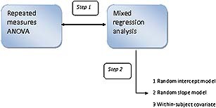
Graphic illustration of the applied models. Step 1 represents the comparison of the repeated measures of ANOVA model with mixed regression analysis with averaged data across trials. Step 2 demonstrates the advantages of mixed regression using single‐trial data.

For the mixed regression analyses the same latency ranges were used as for the ANOVA method. The maximum amplitudes per trial per person were the dependent variables. Aside from intensity and trial, age, absolute stimulus intensity level of the sensation threshold and the pain threshold were included as covariates in this model. Gender was included as a between‐subject variable. The covariates were centred (the sample mean was subtracted from each individual score) (Van Breukelen and Van Dijk, 2007). The rationale for these covariates and between‐subject variables comes from studies that show a relation between these variables and pain or ERP (McDowell et al., 2003; Vallerand and Polomano, 2000) Thus, intensity, trial, age, gender and absolute stimulus intensity level of the sensation threshold and pain threshold were the independent variables (fixed factors). In this model, the intercept was allowed to vary randomly between subjects in order to accommodate interpersonal differences in average ERP. Also, the slopes of intensity and trial were allowed to vary randomly in order to accommodate interpersonal differences in effects of intensity and trial. The analyses were done separately for each component and cranial location. A description of the full mixed regression model is given in the Appendix.

All statistical analyses were performed with SPSS 15.0. All two‐tailed p‐values ≤ 0.007 (Bonferroni correction for the number of cranial locations, i.e. seven) were considered as statistically significant.

Results

Step 1: Repeated measures of ANOVA versus mixed regression

Of the 85 subjects, 29 were excluded due to excessive eye movements, resulting in 56 analyzable sets of participant data. The group consisted of 21 men (37.5%) and 35 women (62.5%). The mean age of the participants was 35 years [standard deviation (SD) = 13.40]. Figure 2a shows the four components of interest in this study: N1, P1, N2 and P2 at Cz, averaged across all 56 subjects and all trials without EOG activity. Visual inspection of Figure 2a indicates that the intensities have different amplitudes: as the intensity increases so does the peak amplitude. Figure 2b shows the averages per block of 10 successive trials for Cz at the strongest stimulus intensity. Figure 2b indicates that as the block increases, the peak amplitude decreases in a non‐linear fashion, suggesting habituation. The difference between the first and second block is larger than the difference between the second and third block. Figure 3 shows the averaged maximum peak amplitudes per intensity of the P2‐component at Cz. Figure displays a combination of the intensity and block effects of Figures 2 and 2b.

Figure 2.

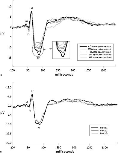
(a) Grand average per stimulus intensity. (b) Grand average per block.

Figure 3.

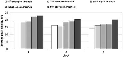
Block averages per intensity on CzP2.

For the comparison of repeated measures of ANOVA and the mixed regression technique, a simple model, following a three (block) by five (intensity) within‐subject design, was chosen. For the sake of simplicity, no covariates were included into the analyses. In order to show that mixed regression analysis produces comparable results to repeated measures of ANOVA, the mixed regression model was adapted in such a way that it most resembled the repeated measures of ANOVA. This meant that the same cases were included (56 out of 85 cases), the same averaged blocks of trials and the same parameters were included in the model. Furthermore, since in repeated measures of ANOVA polynomial contrasts are used, a linear and quadratic contrast for the within‐subject variables intensity and block were included in the mixed regression model. The cubic and quadratic contrasts for intensity were not included in the mixed regression model since significant effects of these contrasts were not expected and these contrasts have no clinical (physiological) meaning. Finally, a Compound Symmetry Heterogeneous (CSH) covariance structure was chosen in the mixed regression analyses as a compromise between compound symmetry (which is close to the sphericity assumption of the univariate ANOVA method for repeated measures) and unstructured (which is equivalent to the assumption made by the multivariate ANOVA method). CSH means that the correlation between repeated measures is the same for each pair of repeated measures, but that the variance may differ between the repeated measures, which implies that the covariances may also differ between pairs.1

The p‐values of the linear and quadratic contrasts for the within‐subject variables (intensity and block) are depicted in Table 1. Table 1 shows overall highly comparable results in the sense of statistically significant and marginally significant effects. No significant interactions between intensity and block were found and therefore these effects are not shown in Table 1. Due to the centred coding of linear and quadratic contrasts, the interaction terms were orthogonal to the main effects.

Table 1.

Comparison of p‐values between repeated measures of ANOVA and multilevel analysis

Location		Contrast	ANOVA (intensity)	Multilevel (intensity)	ANOVA (Block)	Multilevel (Block)
Fz	N1	Linear	p < 0.001	p < 0.001	p = 0.561	p = 0.517
		quadratic	p = 0.052	p = 0.044	p = 0.617	p = 0.596
	P1	Linear	p = 0.145	p = 0.043	p = 0.031	p = 0.008
		quadratic	p = 0.812	p = 0.922	p = 0.247	p = 0.233
	N2	Linear	p < 0.001	p < 0.001	p < 0.001	p < 0.001
		quadratic	p = 0.006	p = 0.030	p = 0.418	p = 0.150
	P2	Linear	p < 0.001	p < 0.001	p < 0.001	p < 0.001
		quadratic	p = 0.194	p = 0.107	p = 0.184	p = 0.300
Cz	N1	Linear	p = 0.061	p = 0.051	p = 0.703	p = 0.736
		quadratic	p = 0.085	p = 0.075	p = 0.723	p = 0.678
	P1	Linear	p = 0.313	p = 0.214	p = 0.377	p = 0.338
		quadratic	p = 0.361	p = 0.640	p = 0.656	p = 0.494
	N2	Linear	p = 0.006	p = 0.001	p < 0.001	p < 0.001
		quadratic	p < 0.001	p = 0.030	p = 0.030	p = 0.140
	P2	Linear	p < 0.001	p < 0.001	p < 0.001	p < 0.001
		quadratic	p = 0.194	p = 0.264	p = 0.080	p = 0.090
Pz	N1	Linear	p = 0.021	p = 0.023	p = 0.449	p = 0.325
		quadratic	p = 0.459	p = 0.575	p = 0.861	p = 0.812
	P1	Linear	p = 0.014	p = 0.003	p = 0.879	p = 0.817
		quadratic	p = 0.186	p = 0.249	p = 0.838	p = 0.901
	N2	Linear	p = 0.692	p = 0.721	p < 0.001	p < 0.001
		quadratic	p = 0.054	p = 0.028	p = 0.486	p = 0.564
	P2	Linear	p < 0.001	p < 0.001	p < 0.001	p < 0.001
		quadratic	p = 0.150	p = 0.135	p = 0.855	p = 0.916

Note: The linear and quadratic effects of intensity and block are depicted. Significant effects (p < 0.007) are displayed in bold and marginally (p <0.05) significant effects are displayed in italics. Results for the other cranial locations showed the same comparable results and are available upon request.

In sum, the comparison of ANOVA repeated measures and mixed regression analyses shows that these two methods can produce comparable results.

Step 2: The advantages of the mixed regression technique

The advantages of the mixed regression technique are demonstrated in three parts. First, single trials are introduced in the analyses. Then random slopes are added to the model and finally a within‐subject covariate is tested.

In mixed regression all valid trials from all participants can be included. This resulted in 85 analyzable cases of which 33 (38.8%) were men and 52 (61.2%) women. T‐Tests and a chi‐square test showed that the 29 extra participants did not differ from the 56 participants in the previous ANOVA/mixed regression analyses with respect to peak amplitude (mean of all valid trials) (p > 0.100), absolute pain threshold (p = 0.972), absolute sensation threshold (p = 0.940), age (p = 0.971) or gender (p = 0.793). Figure 4 displays the trial averages per intensity. It shows saw‐toothed‐like curves caused by the semi‐random presentation of the five intensities (which causes the successive points on the curve for a given intensity to be based on different persons) as well as by intra‐individual variation. Furthermore, an overall decrease over trials is visible.

Figure 4.

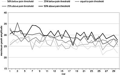
P2 peak amplitude averages at Cz per trial.

Random intercept models

The model consisted of the peak amplitude (N1, P1, N2, P2 components) as dependent variable while intensity_linear, trial_linear, trial_quadratic, trial_inverse, age, gender, absolute sensation threshold and absolute pain threshold served as independent variables. Trial_inverse, computed as (1/trialnr), was included to test for non‐linear habituation effects, that is, for a decrease of peak amplitude which is strong at the start of a subject's session and gets smaller and smaller over the course of the session. Except for trial_quadratic and trial_inverse, all predictors were centred (for details, see the model in the Appendix). Given that no significant block × intensity interactions were found in the analyses of the first hypothesis, no interactions were included in these analyses. Since the number of repeated measures was now 150 (trials) instead of 15 as before, the most general covariance structure that could be fitted was ARMA(1.1), which can handle both white noise (measurement error) and colored noise (AR1, MA1). The intercept was allowed to vary randomly. The goodness‐of‐fit of that covariance structure was significantly better than that of its competitors Compound Symmetry (CS) and AR1. The results of the analyses are displayed in Table 2.

Table 2.

The estimates (B), standard errors (SE) and p‐values for the linear, quadratic and inverse trial effect on Fz, Cz , Pz, C4, C3, T3 and T4

Location		Linear	Quadric	Inverse
Fz	N1	B = −0.002, SE = 0.003, p = 0.560	B = −6E–005, SE = 6.8E–005, p = 0.374	B = −1.80, SE = 1.23, p = 0.144
	P1	B = −0.006, SE = 0.004, p = 0.153	B = −2E–005, SE = 8.2E–005, p = 0.822	B = 1.69, SE = 1.44, p = 0.240
	N2	B = 0.021, SE = 0.004, p < 0.001	B = −0.0002, SE = 8.7E–005, p = 0.009	B = 3.82, SE = 1.58, p = 0.016
	P2	B = −0.012, SE = 0.004, p < 0.001	B = 9.6E–006, SE = 8.8E–005, p = 0.913	B = 4.08, SE = 1.62, p = 0.012
Cz	N1	B = −0.004, SE = 0.003, p = 0.196	B = 5.6E–005, SE = 6.6E–005, p = 0.394	B = −3.49, SE = 1.19, p = 0.003
	P1	B = 0.007, SE = 0.035, p = 0.038	B = −0.00013, SE = 7.5E–005, p = 0.082	B = −1.86, SE = 1.33, p = 0.126
	N2	B = 0.040, SE = 0.004, p < 0.001	B = −0.0003, SE = 8.8E–005, p < 0.001	B = −2.51, SE = 1.56, p = 0.108
	P2	B = −0.025, SE = 0.005, p < 0.001	B = 2.0E–005, SE = 9.9E–005, p = 0.837	B = 2.44, SE = 1.65, p = 0.140
Pz	N1	B = −0.002, SE = 0.003, p = 0.553	B = 2.6E–005, SE = 8.6E–005, p = 0.697	B = −1.14, SE = 1.20, p = 0.344
	P1	B = 0.006, SE = 0.005, p = 0.288	B = −0.0002, SE = 9.7E–005, p = 0.056	B = −0.36, SE = 1.31, p = 0.782
	N2	B = 0.016, SE = 0.004, p < 0.001	B = −0.0001, SE = 8.1E–005, p = 0.142	B = −1.07, SE = 1.45, p = 0.464
	P2	B = −0.013, SE = 0.005, p = 0.008	B = −5.0E–005, SE = 9.4E–005, p = 0.619	B = 2.68, SE = 1.60, p = 0.094
C3	N1	B = −0.002, SE = 0.003, p = 0.419	B = −9.0E–005, SE = 5.8E–005, p = 0.125	B = −2.07, SE = 1.03, p = 0.045
	P1	B = 0.001, SE = 0.004, p = 0.710	B = −0.0002, SE = 7.4E–005, p = 0.042	B = 0.77, SE = 1.22, p = 0.527
	N2	B = 0.027, SE = 0.004, p < 0.001	B = −0.0003, SE = 7.7E–005, p = 0.001	B = −1.11, SE = 1.33, p = 0.407
	P2	B = −0.017, SE = 0.005, p < 0.001	B = −3.0E–005, SE = 8.4E–005, p = 0.761	B = 4.89, SE = 1.41, p = 0.001
C4	N1	B = −0.011, SE = 0.003, p = 0.001	B = −0.0001, SE = 6.4E–005, p = 0.001	B = −1.20, SE = 1.11, p = 0.282
	P1	B = 0.021, SE = 0.005, p < 0.001	B = −0.0001, SE = 8.7E–005, p = 0.137	B = −1.81, SE = 1.30, p = 0.137
	N2	B = 0.030, SE = 0.004, p < 0.001	B = −0.0002, SE = 7.8E–005, p = 0.004	B = −1.96, SE = 1.38, p = 0.153
	P2	B = −0.018, SE = 0.006, p = 0.001	B = 8.1E–005, SE = 9.9E–005, p = 0.417	B = 3.64, SE = 1.51, p = 0.016
T3	N1	B = 0.013, SE = 0.004, p = 0.003	B = −0.0003, SE = 7.3E–005, p <0.001	B = −2.83 SE = 1.00, p = 0.005
	P1	B = −0.013, SE = 0.004, p = 0.002	B = −0.0001, SE = 7.1E–005, p = 0.045	B = −0.87, SE = 1.02, p = 0.394
	N2	B = 0.031, SE = 0.006, p < 0.001	B = −0.0003, SE = 9.4E–005, p = 0.001	B = −3.35, SE = 1.26, p = 0.008
	P2	B = −0.029, SE = 0.005, p < 0.001	B = 0.0004, SE = 8.2E–005, p <0.001	B = 1.22, SE = 1.23, p = 0.321
T4	N1	B = 0.016, SE = 0.004, p < 0.001	B = −0.0002, SE = 7.6E–006, p = 0.009	B = 0.26, SE = 1.55, p = 0.823
	P1	B = 0.003, SE = 0.004, p = 0.461	B = −0.0001, SE = 7.3E–005, p = 0.076	B = −0.46, SE = 1.18, p = 0.706
	N2	B = 0.028, SE = 0.006, p < 0.001	B = −0.0002, SE = 0.00011, p = 0.053	B = −3.50, SE = 1.45, p = 0.016
	P2	B = −0.023, SE = 0.005, p < 0.001	B = −0.0003, SE = 9.6E–005, p = 0.004	B = 3.14, SE = 1.48, p = 0.034

Note: Significant (p < 0.007) effects are displayed in bold and marginally (p < 0.05) significant effects are displayed in italics.

The results demonstrate that the linear, quadratic and inverse effect of trial are statistically significant at multiple cranial locations and components. In order to interpret the size of the effects (B‐values) it should be kept in mind that trial linear runs from −75 to +75, trial quadratic runs from zero to +5625 and trial inverse is coded from one to almost zero. This means that the absolute B‐values cannot be compared to each other. The results show that the linear effect of trials is the strongest over all locations in terms of p‐value. Also the quadratic effect is significant at multiple locations, especially on the N2 component. In addition to the linear and quadratic effect, the inverse effect is significant at CzN1, C3P2 and T3N1.

Furthermore, although not displayed in Table 2, a significant effect of intensity (linear) was found on all components at all locations except for the N2 component at Pz and the N1 and P1 component at T3, T4 and C3. This was overall in accordance with the results of the previous analysis (except for CzP1 and C4P1). A significant effect for age was found on the P2‐component at Cz and Pz. The other covariates did not show a significant effect on the amplitude of the ERP components.

In sum, these analyses demonstrated that the single trials of ERP data differ from each other in that the amplitudes decrease over time. This decrement is a combination of a linear, a quadratic and an inverse trend.

Random slope models

Next, random slopes were added to the model. The random slopes that were included in this model were a random slope for intensity, a random slope for trial_linear and a random slope for trial_inverse. A random slope for trial_quadric was initially also included but dropped in view of non‐significance or convergence problems. The four random effects (three slopes and one intercept) were initially allowed to correlate with each other (giving 10 unknown covariance parameters). In case of convergence problems that could not be solved by dropping the random slope for trial_quadric, random effects were assumed to be uncorrelated, giving four instead of 10, or three instead of six, covariance parameters. Furthermore, since no significant autocorrelation was found anymore after adding random effects, the repeated measures covariance structure was reduced to Scaled Identity (white noise). The resulting fixed effects (B values) of the independent variables were highly similar to the results of the analyses without random effects. The resulting fixed effects and random effect variances are shown in Table 3, showing significant intercept variance (σ²) at all locations and all components.

Table 3.

The fixed effects B and the variances of the random effects σ² on Fz, Cz, Pz, C3, C4, T3 and T4 with their standard errors (SE) between brackets

Location	Intercept		Intensity		Trial linear		Trial inverse
	Fixed	Random	Fixed	Random	Fixed	Random	Fixed	Random
Fz N1	B = −9.13, SE = 0.40	σ2 = 103.91, SE = 1.40	B = −0.31, SE = 0.07	σ2 = 0.07, SE = 0.07	B = −0.002, SE =0.003	σ2 = 0.0002, SE = 0.0001	B = −1.90, SE = 1.66	σ2 = 99.38, SE = 31.86
P1	B = 10.82, SE = 0.66	σ2 = 31.33, SE = 5.25	B = 0.19, SE = 0.11	σ2 = 0.52, SE = 0.16	B = −0.006, SE = 0.004	σ2 = 0.0006, SE = 0.0001	B = 2.09, SE = 1.93	σ2 = 134.93, SE = 47.63
N2	B = −14.17, SE = 0.65	σ2 = 29.93, SE = 5.14	B = −0.37, SE = 0.10	σ2 = 0.31, SE = 0.14	B = 0.02, SE = 0.004	σ2 = 0.0005, SE = 0.0002	B = 3.43, SE = 2.21	σ2 = 180.92, SE = 58.45
P2	B = 19.86, SE = 0.69	σ2 = 33.34, SE = 5.63	B = 0.79, SE = 0.10	σ2 = 0.16, SE = 0.12	B = −0.01, SE = 0.004	σ2 = 0.0003, SE = 0.0002	B = 4.31, SE = 2.14	σ2 = 145.95, SE = 52.29
Cz N1	B = −8.46, SE = 0.40	σ2 = 10.73, SE = 1.88	B = −0.12, SE = 0.08	σ2 = 0.21, SE = 0.08	B = −0.004, SE = 0.003	σ2 = 0.0005, SE = 0.0002	B = −3.54, SE = 1.45	σ2 = 56.35, SE = 24.52
P1	B = 9.63, SE = 0.59	σ2 = 25.17, SE = 4.23	B = −0.35, SE = 0.11	σ2 = 0.54, SE = 0.15	B = 0.007, SE = 0.004	σ2 = 0.0005, SE = 0.0002	B = −1.89, SE = 1.67	σ2 = 84.66, SE = 32.58
N2	B = −16.02, SE = 0.80	σ2 = 47.75, SE = 7.97	B = −0.34, SE = 0.12	σ2 = 0.67, SE = 0.19	B = 0.34, SE = 0.004	σ2 = 0.0006, SE = 0.0002	B = −2.71, SE = 1.75	σ2 = 56.05, SE = 33.81
P2	B = 27.67, SE = 0.83	σ2 = 50.20, SE = 8.55	B = 1.28, SE = 0.08	—	B = −0.03, SE = 0.006	σ2 = 0.002, SE = 00004	B = 2.39, SE = 2.02	σ2 = 104.51, SE = 45.64
Pz N1	B = −6.82, SE = 0.34	σ2 = 4.37, SE = 1.02	B = 0.21, SE = 0.08	—	B = −0.005, SE = 0.004	σ2 = 0.0003, SE = 0.0001	B = −3.11, SE = 1.45	σ2 = 5.86, SE = 16.88
P1	B = 12.08, SE = 0.59	σ2 = 25.47, SE = 4.27	B = 0.27, SE = 0.09	σ2 = 0.24, SE = 0.10	B = 0.006, SE = 0.004	σ2 = 0.0007, SE = 0.0002	B = −0.57, SE = 1.64	σ2 = 82.08, SE = 31.25
N2	B = −11.06, SE = 0.58	σ2 = 23.41, SE = 4.00	B = −0.07, SE = 0.09	σ2 = 0.22, SE = 0.11	B = 0.02, SE = 0.004	σ2 = 0.0006, SE = 0.0002	B = −0.94, SE = 1.77	σ2 = 80.76, SE = 33.62
P2	B = 25.17, SE = 0.77	σ2 = 43.14, SE = 7.21	B = 1.20, SE = 0.10	σ2 = 0.29, SE = 0.14	B = −0.01, SE = 0.005	σ2 = 0.001, SE = 0.0003	B = 2.25, SE = 1.96	σ2 = 101.09, SE = 41.44
C3 N1	B = −7.27 (0.30)	σ2 = 5.68, SE = 1.01	B = −0.03, SE = 0.06	σ2 = 0.02, SE = 0.05	B = −0.002, SE = 0.003	σ2 = 0.0002, SE = 0.0001	B = −2.09, SE = 1.02	—
P1	B = 10.87 (0.55)	σ2 = 22.05, SE = 3.68	B = −0.04, SE = 0.09	σ2 = 0.32, SE = 0.11	B = 0.001, SE = 0.004	σ2 = 0.0006, SE = 0.0002	B = 0.71, SE = 1.38	σ2 = 37.59, SE = 20.27
N2	B = −14.66 (0.64)	σ2 = 29.89, SE = 5.05	B = −0.33, SE = 0.09	σ2 = 0.22, SE = 0.09	B = 0.025, SE = 0.004	σ2 = 0.0006, SE = 0.0002	B = −1.45, SE = 1.53	σ2 = 46.14, SE = 26.89
P2	B = 23.04 (0.76)	σ2 = 42.49, SE = 7.12	B = 0.89, SE = 0.10	σ2 = 0.39, SE = 0.13	B = −0.02, SE = 0.004	σ2 = 0.0009, SE = 0.0002	B = 4.53, SE = 1.79	σ2 = 95.40, SE = 35.86
C4 N1	B = −9.25, SE = 0.49	σ2 = 16.63, SE = 2.84	B = −0.31, SE = 0.09	σ2 = 0.36, SE = 0.11	B = 0.011, SE = 0.003	σ2 = 0.0002, SE = 0.0009	B = −1.18, SE = 1.26	σ2 = 30.57, SE = 17.69
P1	B = 7.23, SE = 0.72	σ2 = 37.20, SE = 6.22	B = −0.34, SE = 0.12	σ2 = 0.78, SE = 0.19	B = 0.022, SE = 0.004	σ2 = 0.0007, SE = 0.0002	B = −1.71, SE = 1.58	σ2 = 70.58 , SE = 28.57
N2	B = −14.64, SE = 0.72	σ2 = 36.87, SE = 6.25	B = −0.36, SE = 0.11	σ2 = 0.47, SE = 0.15	B = −0.03, SE = 0.003	σ2 = 0.0002, SE = 0.0001	B = −1.84, SE = 1.68	σ2 = 73.26 , SE = 31.16
P2	B = 23.08, SE = 0.85	σ2 = 51.99, SE = 8.71	B = 0.83, SE = 0.08	—	B = −0.018, SE = 0.005	σ2 = 0.001, SE = 0.0003	B = 3.29, SE = 2.05	σ2 = 150.46, SE = 47.03
T3 N1	B = −8.88, SE = 0.46	σ2 = 15.44, SE = 2.61	B = 0.03, SE = 0.05	—	B = 0.01, SE = 0.004	σ2 = 0.001, SE = 0.0002	B = −3.10, SE = 1.29	σ2 = 57.43, SE = 20.11
P1	B = 8.78, SE = 0.43	σ2 = 12.98, SE = 2.22	B = −0.03, SE = 0.07	σ2 = 0.11, SE = 0.05	B = −0.02, SE = 0.004	σ2 = 0.0007, SE = 0.0002	B = −0.56, SE = 1.33	σ2 = 61.17, SE = 19.33
N2	B = −15.92, SE = 0.63	σ2 = 29.55, SE = 5.02	B = −0.33, SE = 0.07	σ2 = 0.04, SE = 0.06	B = 0.03, SE = 0.005	σ2 = 0.001, SE = 0.0003	B = −4.39, SE = 1.87	σ2 = 153.10, SE = 41.46
P2	B = 16.93, SE = 0.56	σ2 = 23.24, SE = 3.99	B = 0.33, SE = 0.07	σ2 = 0.15, SE = 0.07	B = −0.027, SE = 0.005	σ2 = 0.001, SE = 0.0003	B = 2.04, SE = 1.78	σ2 = 130.18, SE = 36.89
T4 N1	B = −9.54, SE = 0.51	σ2 = 18.28, SE = 3.13	B = −0.04, SE = 0.07	σ2 = 0.09, SE = 0.06	B = 0.015, SE = 0.004	σ2 = 0.0008, SE = 0.0002	B = 0.16, SE =1.41	σ2 = 55.12, SE = 23.10
P1	B = 6.25, SE = 0.51	σ2 = 18.07, SE = 3.09	B = −0.12, SE = 0.08	σ2 = 0.17, SE = 0.08	B = 0.003, SE = 0.003	σ2 = 0.0005, SE = 0.0002	B = −0.02, SE = 1.45	σ2 = 58.81, SE = 25.16
N2	B = −16.38, SE = 0.78	σ2 = 46.07, SE = 7.76	B = −0.38, SE = 0.08	σ2 = 0.12, SE = 0.09	B = 0.03, SE = 0.005	σ2 = 0.002, SE = 0.0003	B = −4.03, SE = 2.28	σ2 = 243.97, SE = 68.73
P2	B = 16.61, SE = 0.62	σ2 = 27.13, SE = 4.66	B = 0.32, SE = 0.10	σ2 = 0.31, SE = 0.13	B = −0.02, SE = 0.005	σ2 = 0.001, SE = 0.0003	B = 4.32, SE = 2.19	σ2 = 201.18, SE = 55.67

Note : Significance test statistics are computed as B/SE for fixed effects, and σ²/ SE for random effect variances, and approximately standard normally distributed (Z ) under the null hypothesis.For fixed effects, Z > 2.681or < −2.681 is significant at the 0.007 level (Bonferroni corrected for seven locations). For random effect variances, Z > 2.462 is significant at the 0.007 level since variances cannot be negative and are therefore tested one‐sided.

—, variance component could not be estimated and was reported to be redundant, and was therefore set at zero.

The slope variance of intensity is significant on some components of the central line (FzP1, CZN1, CzP1, CzN2) and C3P1, C3P2 C4N1, C4P1 and C4N2 implying inter‐individual differences in the effect of intensity on ERP. The five intensities presented in the protocol were set relative to the individual difference in absolute sensation threshold and pain threshold (see the section Materials and methods, subsection Stimuli). This means that the difference between the intensities was not equal for all subjects. However, the individual differences in the effect of intensity cannot be explained by these individual differences in absolute stimulus intensities, since a post hoc analysis showed the slope variance to be still significant when using absolute intensity instead of relative intensity as predictor in the mixed regression model.

The slope variance of trial_linear is significant on all locations and components except for FzN1, FzP2, C3N1, C4N1 and C4N2. The slope variance of trial_inverse is significant on all components of Fz and T3, on the N2‐component of T4 and the P2‐components of C3, C4 and T4 and on none of the components of Cz and Pz.

These analyses demonstrated that there are individual differences in the effects of intensity and trial on the ERP, which can be quantified in terms of between‐subject variances in within‐subject slopes for the regression of ERP on intensity and trial. This is a more refined way to study individual differences compared to repeated measures of ANOVA of block averages.

Within‐subject covariate

The final step was to include a within‐subject covariate: intensity of the previous trial. This covariate was centred and then included as main effect and as part of an interaction term with intensity of the current trial. Random effects in this model were as in the previous model. The results showed that the main effect of the intensity of the previous trial was not significant at any of the cranial locations and ERP components. The interaction between the intensity of the previous trial and the intensity of the current trial was significant on C3N2 (p = 0.003). Furthermore, on the other components of C3 this interaction was marginally significant (p‐values between 0.05 and 0.007). Finally, the results of the other independent variables (intensity, trial, age, gender, sensation and pain threshold) remained essentially the same after including the within‐subject covariate

In sum, the large amount of results presented in this section demonstrate that (i) mixed regression analysis produces similar results compared to the more traditional repeated measures of ANOVA, (ii) mixed regression analyses demonstrate that not only the linear effect of trial is significant, but also the quadratic and inverse effect and that these effects were mostly significant on the lateral cranial locations (see Table 2), (iii) the intercept and slopes of intensity and trial varied significantly between individuals and (iv) the within‐subject covariate, stimulus of the previous intensity, was significant in interaction with the intensity of the present stimulus on C3N2.

Discussion

The aim of this study was to demonstrate that the mixed regression technique is a flexible and appropriate method for analyzing ERPs and that it has some important advantages over the traditional way of analysis (with repeated measures of ANOVA).

Before demonstrating the advantages of the mixed regression technique, confirmation was provided that the mixed regression technique can provide the same results as repeated measures of ANOVA. The p‐values of the two analysis techniques were highly comparable. The small differences can be explained by the fact that repeated measures of ANOVA uses an unstructured covariance structure and that for the mixed regression analyses a compound symmetry (heterogeneous) covariance structure was chosen2 which is somewhat less general than unstructured. Although assuming an unstructured covariance matrix is often preferable (since it is the most flexible covariance structure) and so repeated measures of ANOVA might seem better, there are some strong arguments in favour of mixed regression analysis

Therefore, an attempt was made to show that the mixed regression technique has some important advantages over repeated measures of AVOVA. A first advantage of the mixed regression technique is that single trial data can be used in the analyses. This not only allows inclusion of subjects with missing data, as mentioned earlier (which in turn increases the power and reduces the risk of selection bias), but also allows the study of time (trial) effects with any kind of function of trial number, including an inverse (1/trial) function. The results show that in addition to a strong linear trial effect and a fairly strong quadratic trial effect, the inverse trial effect was also significant at different components and locations. Furthermore, there were several marginally significant effects of the inverse trial effect (p‐values between 0.05 and 0.007). These results imply that the peak amplitudes of the ERP decrease over time (habituation) but that the way in which they decrease cannot merely be expressed in polynomial (linear and quadratic) contrasts. This is in accordance with the consensus that pain habituates in a non‐linear fashion (Milne et al., 1991).

Another advantage is that in mixed regression analysis it is possible to study individual differences in the within‐subject variance. In practice, this means that individual differences in the effect of intensity and trial on the cortical processing of stimuli can be investigated. These subject × time and subject × intensity interactions are represented as random slopes. In the analyses, a random intercept, random slope for intensity and two random slopes for trial (linear and inverse) were included. The results showed strong intercept variance, representing differences in mean amplitude between the subjects. The significant slope variance for intensity represents individual differences in the effect of intensity. Furthermore, significant slope variance for trial linear and trial inverse was found, implying individual differences in the habituation to repeated measures. This is an interesting finding, because these individual differences in habituation might in part explain individual differences in the response to pain in general which in turn might explain the development of chronic pain complaints (Valeriani et al., 2003). These results can be used to form and test new hypotheses to explain these individual differences.

Finally, because single trial data was used in the analyses, covariates that vary over trials (within‐subject covariate) can be investigated. In this study, the intensity of the previous trial was included in the model because of the semi‐random presentation of the intensities in the paradigm. Our hypothesis was that the intensity of the previous stimulus influences the cortical reaction of the present stimulus. Moreover, it was expected that an interaction between the intensity of the current stimulus and the intensity of the previous stimulus (difference in intensity) would influence the cortical response to the current stimulus. The results did not confirm these hypotheses. No main effect of the intensity of the previous stimulus was found. However, a significant interaction effect was found on the N2‐component of C3, meaning that the effect of the intensity of the current stimulus on the ERP amplitude is dependent of the intensity of the previous stimulus. Also marginally significant interaction effects (p‐values between 0.05 and 0.007) were found on the other components of C3. This might imply that this area is involved in the comparison of past and present intensities, but further research will have to confirm this.

Naturally, fine‐tuning of this technique is necessary. For instance, relatively simple techniques for filtering and detection of components were used. The mixed regression analysis technique can also be used in combination with other techniques of component identification such as Principal Component Analysis or Wavelet analysis. Furthermore, in this study, the inverse function was calculated by dividing one by the trial number. Of course there are other ways to calculate an inverse function which might even better fit the data.

In conclusion, this article has demonstrated on a theoretical as well as a practical level that the mixed regression technique offers important advantages for ERP research. The model given in this study can easily be adapted to different ERP paradigms (e.g. Oddball paradigms) and research questions by including different independent variables and different random effects. Using mixed regression analysis as a statistical technique in ERP research will advance the unravelling of mechanisms underlying the ERP.

Declaration of interest statement

The authors have no competing interests

The full mixed regression model PTSD

Y_ti = β₀ + β₁ intensity_liner  + β₂ trial_liner  + β₃ trial_quad  + β₄ trial_invers  + β₅ age + β₆ gender + β₇ absolute sensation threshold + β₈ absolute pain threshold + β₉ intensity_liner previous trial^†  + β₁₀ intensity_liner  × intensity_liner previous trial^†  + e_ti + u _0i + u _1i intensity_liner + u _2i trial_liner + u _3i trial_inverse

^†The intensity of the previous trial was not included until the last step of the analyses.

Where:

• t = time point (1–150),

• i = subject

• Intensity = −2 = −50%,

• –1 = −25%,

• 0 = 0%,

• 1 = 25% and 2 = 50%,

• Trial = 150 trial numbers,

• centred from −74.5 to +74.5,

• Age = centred continuous variable in years,

• Gender = dichotomous variable,

• –1 = man,

• 1 = woman,

• Absolute sensation threshold = centred continuous variable in mA,

• Absolute pain threshold = centred continuous variable in mA,

• Intensity previous trial = −2 = −50%,

• –1 = −25%,

• 0 = 0%,

• 1 = 25% and 2 = 50%,

• e_ti = error variance for subject i at time point t. which is assumed to follow a ARMA(1.1) process, which includes as a special case autoregression (AR1) plus white noise (measurement error), among others. (The analyses of this study demonstrated overall 0 > phi > rho, validating the choice of covariance structure.)

• u _0i = personal deviation from the average intercept β ₀

• u _1i = personal deviation from the average slope

• β ₁ of intensity_liner u _2i = personal deviation from the average slope β ₂ of trial_liner

• u _4i = personal deviation from the average slope β ₂ of trial_linverse

The four random person effects are allowed to correlate with each other.

This model must be interpreted as follows:

• β ₀ = the outcome mean (Amplitude) for the intensity equal to the pain threshold (intensity = 0) at trial number 75 for a subject with a mean age, mean absolute sensation threshold and mean absolute pain threshold.

• β ₁ = the mean difference between the adjacent intensities

• β ₂ = the mean change over trials according to the linear part of the trend

• β ₃ = the quadratic trial effect

• β ₄ = the inverse trial effect

• β ₅ = the mean change in amplitude per year

• β ₆ = half the mean difference between men and women

• β ₇ = the relation between the absolute sensation threshold and the amplitude of the component

• β ₈ = the relation between the absolute pain threshold and the amplitude of the component

• β ₉ = the relation between the intensity of the previous trial and the amplitude of the present trial.

• β ₁₀ = the effect of the intensity of the previous trial on the difference in amplitude between adjacent intensities (e.g. intensity 2 versus 1, or 1 versus 0) for the current trial.

References

- Becker D.E., Haley D.W., Urena V.M., Yingling C.D. (2000) Pain measurement with evoked potentials: combination of subjective ratings, randomized intensities, and long interstimulus intervals procedures a P300‐like confound. Pain, 84, 37–47. [DOI] [PubMed] [Google Scholar]
- Bostanov V., Kotchoubey B. (2006) The t‐CWT: A new ERP detection and quantification method based on the continuous wavelet transform and Student's t‐statistics. Clinical Neurophysiology, 177, 2627–2644. [DOI] [PubMed] [Google Scholar]
- Bromm B., Meier W. (1984) The intracutaneous stimulus: A new pain model for algesimetric studies. Methods and Findings in Experimental & Clinical Pharmacology, 6, 405–410. [PubMed] [Google Scholar]
- Carrillo‐de‐la‐Peňa M.T. (1992) ERP augmenting/reducing and sensation seeking: A critical review. International Journal of Psychophysiology, 12, 211–220. [DOI] [PubMed] [Google Scholar]
- Chapman R.M., McCrary J.W. (1995) EP Component identification and measurement by principal component analysis. Brain and Cognition, 27, 288–310. [DOI] [PubMed] [Google Scholar]
- Farwell L.A., Martinerie J.M., Bashore T.R., Rapp P.E., Goddard P.H. (1993) Optimal digital filters for long‐latency components of event‐related potentials. Psychophysiology, 30, 306–315. [DOI] [PubMed] [Google Scholar]
- Goldstein H. (1999) Multilevel Statistical Analyses, London, Institution of Education, Multilevel Models Project. http://www.arnoldpublishers.com/support/goldstein.htm. [1 May 2009]
- Granovsky Y., Granot M., Nir R.R., Yarnitsky D. (2008) Objective correlate of subjective pain perception by contact heat‐evoked potentials. Journal of Pain, 9, 53–63. [DOI] [PubMed] [Google Scholar]
- Hansenne M. (2006) Event‐related potentials in psychopathology: Clinical and cognitive perspectives. Psychologica‐Belgica, 46, 5–36. [Google Scholar]
- Hoormann J., Falkenstein M., Schwarzenau P., Hohnsbein J. (1998) Methods for the quantification and statistical testing of ERP differences across conditions. Behavior Research Methods, Instruments, & Computers, 30, 103–109. [Google Scholar]
- Jasper H.H. (1958) The ten‐twenty electrode system of the International Federation. Journal of Electroencephalography Clinical and Neurophysiology, 20, 371–375. [PubMed] [Google Scholar]
- Jung T.P., Makeig S., Westerfield J.T., Courchesne E., Seijnowski T. (2001) Analysis and vizualization of single‐trial event‐related potentials. Human Brain Mapping, 14, 166–185. [DOI] [PMC free article] [PubMed] [Google Scholar]
- Kanda M., Matsuhashi M., Sawamoto N., Oga T., Mima T., Nagamine T., Shibasaki H. (2002) Cortical potentials related to assessment of pain intensity with visual analogue scale (VAS). Clinical Neurophysiology, 113, 1013–1024. [DOI] [PubMed] [Google Scholar]
- Katada E., Sato K., Ojika K., Ueda R. (2004) Cognitive event‐related potentials: Useful clinical information on Alzheimer's disease. Current Alzheimer Research, 1, 63–69. [DOI] [PubMed] [Google Scholar]
- Mazaheri A., Jensen O. (2008) Asymmetric amplitude modulations of brain oscillations generate slow evoked responses. Journal of Neuroscience, 28, 7781–7787. [DOI] [PMC free article] [PubMed] [Google Scholar]
- McDowell K., Kerick S.E., Santa Maria D.L., Hatfield B.D. (2003) Aging, physical activity, and cognitive processing: An examination of P300. Neurobiology of Aging, 24, 579–606. [DOI] [PubMed] [Google Scholar]
- Milne R.J., Kay N.E., Irwin R.J. (1991) Habituation to repeated painful and non‐painful cutaneous stimuli: A quantitative psychophysiological study. Experimental Brain Research, 87, 438–444. [DOI] [PubMed] [Google Scholar]
- Miltner W., Larbig W., Braun C. (1987) Habituation of subjective ratings and event‐related potentials to painful intracutaneous electrical stimulation of the skin. Journal of Psychophysiology, 1, 221–228. [Google Scholar]
- Nikulin V.V., Linkenkaer‐Hansen K., Nolte G., Lemm S., Müller K.R., Ilmoniemi R.J., Curio G. (2007) A novel mechanism for evoked responses in the human brain. European Journal of Neuroscience, 25, 3146–3154. [DOI] [PubMed] [Google Scholar]
- Porjesz B., Rangaswamy M., Kamarajan C., Jones K.A., Padmanabhapillai A., Begleiter H. (2005) The utility of neurophysiological markers in the study of alcoholism. Clinical Neurophysiology, 116, 993–1018. [DOI] [PubMed] [Google Scholar]
- Snijders T., Bosker R. (2000) Multilevel Analysis, London, United Kingdom: Sage Publications. [Google Scholar]
- Spyzou L., Sanei S. (2008) Source localization of event‐related potentials incorporating spatial notch filters. IEEE Transaction, Biomedical Engineering, 55, 2232–2239. [DOI] [PubMed] [Google Scholar]
- Timmermann L., Ploner M., Schmitz F., Baltissen R., Schnitzler A. (2001) Differential coding of pain intensity in the human primary and secondary somatosensory cortex. Journal of Neurophysiology, 86, 1499–1503. [DOI] [PubMed] [Google Scholar]
- Valeriani M., de Tommaso M., Restuccia D., Le Pera D., Guido M., Iannetti GD, Libro G., Truini A., Di Trapani G., Puca F., Tonali P., Cruccu G. (2003) Reduced habituation to experimental pain in migraine patients: A CO2 laser evoked potential study. Pain, 105, 57–64. [DOI] [PubMed] [Google Scholar]
- Vallerand A.H., Polomano R.C. (2000) The relationship of gender to pain. Pain Management Nursing, 1, 8–15. [DOI] [PubMed] [Google Scholar]
- Van Breukelen G.J.P., Van Dijk K.R.A. (2007) Use of covariates in randomized controlled trials. Journal of the International Neuropsychological Society, 13, 903–904. [DOI] [PubMed] [Google Scholar]
- Verbeke G., Molenberghs G. (2000) Linear Mixed Models for Longitudinal Data, New York: Springer. [Google Scholar]
- Woestenburg J.C., Verbaten M.N., van Hees H.H., Slangen J.L. (1983) Single trial ERP estimation in the frequency domain using Orthogonal Polynomial Trend Analyses (OPTA): Estimation of individual habituation. Biological Psychology, 17, 173–191. [DOI] [PubMed] [Google Scholar]
- Zaslansky R., Sprecher E., Tenke C.E., Hemli J.A., Yarnitsky G. (1996) The P300 in evoked potentials. Pain, 66, 39–49. [DOI] [PubMed] [Google Scholar]