A field-based characterization of conductivity in areas of minimal alteration: A case example in the Cascades of northwestern United States

Abstract

The concentration of salts in streams is increasing world-wide making freshwater a declining resource. Developing thresholds for freshwater with low specific conductivity (SC), a measure of dissolved ions in water, may protect high quality resources that are refugia for aquatic life and that dilute downstream waters. In this case example, methods are illustrated for estimating protective levels for streams with low SC. The Cascades in the Pacific Northwest of the United States of America were selected for the case study because a geophysical model indicated that the SC of freshwater streams was likely to be very low. Also, there was an insufficient range in the SC data to accurately derive a criterion using the 2011, US Environmental Protection Agency field-based extirpation concentration distribution method. Instead, background and a regression model were used to estimate chronic and acute SC levels that could extirpate 5% of benthic invertebrate genera. Background SC was estimated at the 25th centile (33 μS/cm) of the measured data and used as the independent variable in a least squares empirical background-to-criterion (B-C) model. Because no comparison could be made with effect levels estimated from paired SC and biological data set from the Cascades, the lower 50% prediction limit (PL) was identified as an example chronic water quality criterion (97 μS/cm). The maximum exposure threshold was estimated at the 90th centile SC of streams meeting the chronic SC level. The example acute SC level was 190 μS/cm. Because paired aquatic life and SC data are often sparse, the B-C method is useful for developing SC criteria for other systems with limited data.

Graphical Abstract

1. Introduction

As human populations have increased, dissolved mineral inputs to streams have increased (ECHC, 2001; Kaushal et al., 2005, 2013, 2018; Cañedo-Argüelles et al., 2013; Anning and Flynn, 2014). However, some streams are remarkably pristine with very low specific conductivity (SC), a measure of the total concentration of dissolved ions. These low SC streams are essential for diluting downstream waters where inputs of dissolved minerals have increased (Merriam et al., 2011; U.S. EPA, 2011a). These low SC ecosystems are also critical habitats for obligate salt-intolerant fish (Griffith et al., 2017), benthic invertebrates (Cormier et al., 2013a), and aquatic plants (Potapova and Charles, 2003; Potapova, 2005). Because increased dissolved minerals can be harmful for aquatic life (U.S. EPA, 2011a; Cañedo-Argüelles et al., 2013; Cormier et al., 2013a), it would be useful to be able to identify areas with low SC and aquatic communities that are vulnerable to changes in ionic loadings.

Streams with potentially low SC can be predicted based on geology, climate, soil, vegetation, topography, and other factors (Olson and Hawkins, 2012). This predicted background can be verified by in-stream measurements of SC in reference locations. In the contiguous United States of America (USA), low SC systems occur most commonly in the Pacific Northwest and the eastern half of the country where rainfall is plentiful (Olson and Hawkins, 2012; Anning and Flynn, 2014; Cormier et al., 2018c).

The effect of increased SC has been demonstrated in single species experiments (e.g. Kefford et al., 2004; Kunz et al., 2013; Soucek and Dickinson, 2015; Mount et al., 2016; Erickson et al., 2017; Scheibener, 2017), mesocosm experiments (e.g. Clements and Kotalik, 2016; Sala et al., 2016; Olson and Hawkins, 2017), field experiments (e.g. Wood and Dykes, 2002), and field observational studies (e.g. Pond et al., 2008; Pond, 2010; Cormier et al., 2013b; Dunlop et al., 2015; Vander Laan et al., 2013; Timpano et al., 2015). Studies of the physiological mechanisms of adverse effects demonstrate that at low SC, increases in bicarbonate can interfere with the ionic homeostasis, which includes regulation of the relative concentrations of ions of an organism’s tissues and cells (see Bradley, 2009 for physiological and Griffith, 2017 for molecular reviews). The relative amounts of ions, including sodium and sulfate also appear to affect ion toxicity (Scheibener, 2017). Although death is a commonly used laboratory endpoint, mesocosm (Clements and Kotalik, 2016; Olson and Hawkins, 2017) and field experiments (Wood and Dykes, 2002) have shown that behavioral and other sublethal effects of ionic stress have the potential to lead to population level effects such as species extirpation.

Field-based methods have a number of advantages compared with laboratory methods for estimating protective levels (Gerritsen et al., 2015; Vander Laan et al., 2013; Buchwalter et al., 2017). Field-based methods measure effects from all modes of action that are actually causing harm in the environment in addition to the mortality, growth, and reproductive effects identified in laboratory tests. These include emigration and interactions among organisms such as parasitism, competition, disease, and predation. Also, effects reflect events that occur during narrow windows of life cycles that may not occur in standard tests. For example, spawning, insect emergence, and migration are mediated by sensory, hormonal, and behavioral alterations. Consequently, for substances that naturally occur in the field such as salts (Olson and Hawkins, 2017) and ammonia (Yang et al., 2017), field-based methods measure the full range of effects at all levels of organization and are likely to assess the most susceptible species, relevant effects and life stages.

However, there are disadvantages of using field survey data to develop effect thresholds including, the potential influence of confounders on the stressor-effect relationship (Suter and Cormier 2013) and sufficiently large paired biological and chemical data sets (Cormier et al., 2018c). An additional challenge in pristine ecosystems is that there may not be sufficient numbers of streams with adverse exposure levels to be able to characterize the relationship between exposure and adverse effects. Such a situation was encountered in the Cascades region of the Pacific Northwest, USA. There were few stream samples with SC >300 μS/cm. Therefore, the range of exposure may be too narrow to assess the tolerance ranges of paired benthic invertebrate. Thus, a stressor-response relationship between SC and extirpation of benthic invertebrate genera could not be developed using field data from the Cascades. However, there is an alternative method not dependent on paired biological and chemical data. The method uses a general relationship between the SC level causing extirpation of 5% of benthic invertebrate genera and background SC. This background-to-criterion (B-C) model was constructed from paired SC and the 5th centile SC of distributions of extirpation concentration values (XCD₀₅) from 24 distinct areas in the contiguous United States that exhibited a range of background SC (Cormier et al., 2018a).

The advantage of the B-C method is that paired biological and SC samples are not needed from a large population of streams with a broad range of SC regimes. SC measurements are easier and less expensive to sample than obtaining both SC and paired biological samples. Moreover, the SC data set only needs to be large enough to characterize background SC.

In this paper, a case study from the Cascades in the Pacific Northwest, USA is used to demonstrate how to use the B-C model to estimate an example chronic threshold, a criterion continuous concentration (CCC). It also estimates an example acute threshold, a criterion maximum exposure concentration (CMEC), using only SC data from the region (Cormier et al., 2018b).

2. Methods

2.1. Study area

The Cascades (Level III Ecoregion 4) is a mountainous ecoregion extending from northern California into the central portion of western Washington (Omernik, 1987; U.S. EPA, 2011b) (Fig. 1). A small portion of the Cascades in California is separated from the rest of the ecoregion by the Klamath River Valley. The ecoregion consists of snow-capped and glaciated peaks, steep slopes, stream valleys, active and inactive volcanoes, and elevations mainly between 645 and 2258 m but extending up to 4390 m (Sorenson, 2012). Most of the terrain was glaciated in the past and bedrock and soils are volcanic in origin (U.S. EPA, 2011b).

Fig. 1.

Sampling locations in the EPA-survey, State, and U.S. Geological Survey (USGS) data sets that were used to estimate background specific conductivity (SC) in the Cascades (shaded gray). Sampling locations are color coded by specific SC ranges: green diamonds <30 μS/cm, yellow squares 30–100 μS/cm, and red triangles ≥100 μS/cm. Geodetic reference system = North American Datum (NAD83). Modified from U.S. EPA (2016).

The climate is temperate with an annual average precipitation ranging from 130 to 380 cm, temperatures ranging from −1 °C to 11 °C, and growing season between 30 and 240 days (Sorenson, 2012). Coniferous forests dominate elevations below 3350 m, and alpine meadows and barren areas are more prevalent at higher elevations.

2.2. Analytical methods

2.2.1. Background conductivity

Background SC is the independent variable used to predict a chronic criterion from the B-C model. The background SC was estimated as the 25th centile from the Combined data (EPA-survey, State, and USGS data sets). The 25th centile is a conventional endpoint for estimating background for naturally occurring water quality attributes from mixed data sets and probabilistic data sets (U.S. EPA, 2000). The 75^th centile from best available reference locations has been shown to be comparable to the 25th centile of mixed data sets of SC measurements (U.S. EPA, 2011a).

2.2.2. Chronic and acute effect level

An example CCC was calculated using an estimate of background SC and the B-C model (Cormier et al., 2018a). The selection of the B-C method was based on a decision flowchart also described in this issue (Cormier et al., 2018c). Available data sets for the Cascades did not meet the minimum requirements for data set size or range of SC to calculate a CCC using paired biological and SC data (Fig. 2). Therefore, the CCC was calculated from the B-C model and background SC for the ecoregion using the B-C model and background SC for the Cascades. The lower 50% PL of the mean predicted XCD₀₅ was selected as the CCC as shown in Fig. 2 because there was no independently derived value to compare with the mean predicted XCD₀₅. When the value is derived using large paired data sets of SC and biological data as described by Cormier and Suter (2013a), 25% of calculated CCC values are expected to be less than the lower 50% PL derived with the B-C model. The general steps for calculating the CCC using the B-C model is shown in Fig. 3 and the detailed calculation in the section on Analysis 3.3. An example acute criterion or CMEC was calculated using the CCC and variance of SC measured in streams meeting the CCC (Fig. 3) (Cormier et al., 2018b). R, version 2.12.1, was used for calculating all data analyses including the CCC and CMEC (R Development Core Team, 2011).

Fig. 2.

Process and decision flow chart for the case example for the Cascades. Decision path is highlighted in gray and connected by bold lines. Because there were no suitable paired biological and specific conductivity (SC) data to derive a taxonomic extirpation concentration distribution (XCD) for the Cascades, the SC predicted to result in 5% extirpation (XCD05) was calculated with the background to-criterion (B-C) model at the lower 50% prediction limit (PL). Modified from U.S. EPA (2016).

Fig. 3.

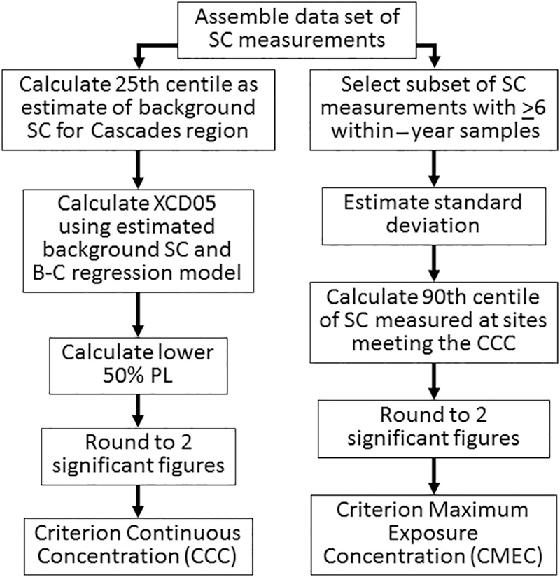
Steps to calculate a CCC using the B-C model and the CMEC as a maximum SC of streams with an annual average SC equal to the CCC.

2.3. General data set description

Water chemistry data previously collected by 4 independent entities were used for analysis. U.S. EPA survey, State, and U.S. Geological Survey (USGS) data sets (Table 1) were combined into two types of data sets. A Combined data set was used to characterize ion composition and water chemistry, characterize background SC, and calculate an example CCC. A Multiple-SC data set was used to estimate the SC variance of streams that was then used to calculate an example CMEC. All stations in the Combined data set included at least one measure of ion concentration or SC. All stations in the Multiple-SC data set included multiple within-year SC samples so that annual variance could be calculated. Data sets are available on the U.S. EPA Environmental Dataset Gateway (https://doi.org/10.23719/1396168).

Table 1.

Sources for data used in the assessment. EPA-Survey, State, and U.S. Geological Survey (USGS) chemistry data sets included in this study. Years indicate the period during which the samples were collected. At least one type of ionic or SC measurement was sampled at each sampling station.

Survey	Years	# of stations	# of samples
EPA-Survey Data	1995−2009	152	152
State Data
Oregon	1990−2014	418	2,511
Washington	1990−2015	121	562
Total (Note: 90 stations with SC)		539	3,073
State: subset ≥ six samples per year, January−December	1990−2015	19	1,111
USGS Targeted Sampling
USGS	1958−2016	282	6,258
USGS Subset: ≥ 6 samples per year, January−December	1959−2014	50	5,019

Different sampling designs and geographic coverages were used by each agency and can affect interpretation of SC statistics. Minor differences in the analytical chemistry methods of individual ions are described in published protocols by each agency which are listed with each data set. However, ionic measurements can be compared across data sets and all SC were measured with a conductivity meter calibrated to 25 °C. When more than one sample was collected at a location, the geometric mean was calculated. Using the geometric mean reduces the potential for a few outliers to influence the estimate of the calculated value. When multiple measurements are used to estimate the standard deviation for calculation of the example CMEC, then measurements were not averaged.

2.3.1. U.S. EPA-Survey data set

All U.S. EPA-Survey samples were collected from first- through fourth-order streams to characterize stream water chemistry (Table 2). The National Rivers and Streams Assessment (NRSA) 2008–2009 data set (U.S. EPA, 2013b), National Wadeable Stream Assessment (NWSA) 2004 data set (U.S. EPA, 2006), and Regional Environmental Monitoring and Assessment Program (EMAP) 1999 data sets (U.S. EPA, 2013a), are based on single random (i.e. probability-based design) samples from June through September. Although, the probability design sampling weights for stream order were not used in the characterization, these samples are not biased as may occur with targeted sampling. Analysis of water chemistry samples followed procedural and quality assurance protocols used by U.S. EPA and EMAP (U.S. EPA, 1987, 1994, 1998, 2001), NWSA (U.S. EPA, 2004a, 2004b, 2006), and NRSA (U.S. EPA, 2009).

Table 2.

Summary of data from EPA-survey samples. Calculated values are means are geometric except for pH values and ion ratios which are arithmetic means. N is the number of stations.

Parameter	N	Minimum	25th	50th	Mean	75th	Maximum
SC (µS/cm)	152	1.56	33.9	44.9	44.8	61.8	205.0
pH (SU)	144	6.17	7.3	7.5	7.5	7.7	9.0
Ca2+ (mg/L)	70	0.04	3.1	4.8	4.7	8.1	22.7
Mg2+ (mg/L)	70	0.03	0.7	1.3	1.2	1.9	8.8
Na+ (mg/L)	70	0.08	2.1	2.8	2.7	4.0	10.4
K+ (mg/L)	70	0.01	0.2	0.5	0.5	0.8	3.2
HCO3− (mg/L)	46	0.46	18.3	26.4	25.4	40.0	132.2
SO42− (mg/L)	121	0.07	0.4	1.0	1.0	2.3	34.3
Cl− (mg/L)	136	0.14	0.6	0.9	0.8	1.1	12.2
HCO3− + SO42−/Cl−	46	3.88	24.5	32.3	50.4	58.4	211.1

Most of these single grab samples have reported SC, alkalinity, hardness, sulfate, chloride, bicarbonate, sodium, calcium, magnesium, and pH, as well as other water quality parameters. Centiles were calculated from the total number of samples.

2.3.2. State data set (U.S. EPA Region 10)

The State data set (Table 3) includes data from the Oregon Department of Environmental Quality (ODEQ) collected between 1990–2014 (ODEQ, 2009) and from the Washington Department of Ecology (WDE) collected between 1990–2015 (WDE, 2014). Monthly sampling was performed throughout the year at many stations. Most samples have reported sulfate, chloride, bicarbonate, and pH. About one-third include SC. Centiles are based on calculated station geometric means except for pH values and ion ratios which are arithmetic means of multiple samples from the same sampling location.

Table 3.

Summary of State data set for the Cascades. Centiles are based on calculated station geometric means except for ion ratios which are arithmetic means. N is the number of stations.

Parameter	N	Minimum	25th	50th	Mean	75th	Maximum
SC (μS/cm)	95	6.8	24.0	32.4	31.9	39.4	125.9
Ca2+ (mg/L)	78	1.0	2.3	3.0	3.7	4.3	1,100
HCO3− (mg/L)	300	7.7	19.9	25.8	27.5	38.0	3,966
SO42− (mg/L)	252	0.1	0.3	0.6	0.8	1.7	36.2
Cl− (mg/L)	315	0.3	0.7	1.0	1.1	1.5	250.0
HCO3− + SO42−/Cl−	203	3.3	18.0	28.2	37.6	46.0	225.7

2.3.3. U.S. Geological Survey (USGS) data set

All USGS samples were collected from first- through fourth-order streams for various research purposes. The USGS survey data set is composed of 6258 water quality samples, from 290 stations within the Cascades (Table 4). Some stations were sampled only once while others were sampled as many as 641 times. The data were collected between 1958 and 2016 during all seasons. Most of the samples have reported SC, alkalinity, hardness, sulfate, chloride, bicarbonate, and pH, as well as other water quality parameters. Analysis of water chemistry samples followed procedural and data quality assurance protocols for USGS data sets (Mueller et al., 1997).

Table 4.

Summary of data for the Cascades from the U.S. Geological Survey (USGS). Calculated means are geometric means except for pH which is an arithmetic mean. N is the number of stations.

Parameter	N	Minimum	25th	50th	Mean	75th	Maximum
SC (μS/cm)	282	3.50	38	53.9	53.6	78.3	370
pH (SU)	274	6.2	7.2	7.5	7.4	7.7	8.7
Ca2+ (mg/L)	5	1.6	1.7	2.1	2.9	5.6	15.7
Mg2+ (mg/L)	158	0.10	0.78	1.39	1.31	2.43	9.08
Na+ (mg/L)	5	1.2	1.2	1.3	1.7	2.5	5.6
K+ (mg/L)	5	0.1	0.2	0.2	0.3	0.5	1.3
HCO3− (mg/L)	57	3.0	29.8	35.0	37.0	51.3	122.0

Eight stations were removed from the parent data set leaving 282 stations. Samples from Lake Paulina and Longmire Meadow were removed because these are mineral springs (Ingebritsen et al., 2014). Samples from ash flows on the flanks of Mt. St. Helens were removed because they exhibited very high SC and were not representative of typical streams in the region. The USGS data set was useful because it included areas of the ecoregion that were underrepresented by samples in the other two data sets.

2.4. Data Set for ionic composition, background SC, and CCC

2.4.1. Combined data set

The U.S. EPA, State, and USGS data set contained 152 stations, 539 (SC at 95) stations, and 282 stations, respectively, and together formed the Combined data set (Table 5). For each station with multiple measurements in a year, the geometric mean SC was calculated. For each station with a single measurement, that value was also included in the Combined data set. The Combined data set was used to characterize the concentrations of the ions in the Cascades. It was also used to characterize the range of SC in the region and to calculate the 25^th centile SC for the region as an estimate of background SC.

Table 5.

Summary of Combined data set. Values are based on geometric means except for pH values and ion ratios which are based on arithmetic means. N is the number of stations.

Parameter	N	Minimum	25th	50th	Mean	75th	Maximum
SC (μS/cm)	529	1.6	32.7	46.4	46.4	66	370
pH (SU)	418	6.2	7.2	7.5	7.4	7.7	9
Ca2+ (mg/L)	153	0.04	2.51	3.59	4.06	6.36	1,100
Mg2+ (mg/L)	228	0.03	0.77	1.34	1.29	2.2	9
Na+ (mg/L)	75	0.08	2.03	2.76	2.59	3.96	10
K+ (mg/L)	75	0.01	0.22	0.49	0.44	0.77	3
HCO3− (mg/L)	403	0.46	20.42	28.04	28.38	40.19	3,966
SO42− (mg/L)	373	0.07	0.34	0.78	0.85	2.17	36
Cl− (mg/L)	451	0.14	0.63	1	1	1.4	250
HCO3− + SO42−/Cl−	249	3.29	18.31	28.6	40	48.5	225.7

2.5. Data to estimate SC standard deviation and CMEC

2.5.1. Multiple-SC data set

The Multiple SC data set was used to estimate the standard deviation value for calculating the CMEC. Stations from the USGS and State data sets were combined to form the Multiple-SC data set because these data sets contained multiple measurements in a year from sampling stations. The Multiple-SC data set was constructed by excluding stations with fewer than six SC measurements throughout the year. At least, one sample during the spring (March to June) and one in the summer (July to October) were also required so that it was more likely that the periods of lower and higher SC would be included in the data set. Some stations were sampled in several years. A rotation year began in July and ended in June. The July to June rotation was selected to align with the natural history of the many salt-intolerant genera that emerge as winged adults before July. The July to June rotation is not essential for this calculation but was selected to allow comparison with methods that use paired biological and chemical samples (Cormier et al., 2018b). Of the 312 rotation-years from the 69 unique stations, the USGS data set contributed 5019 samples from 50 stations, while the State data set contributed 1111 samples from 19 stations.

3. Analysis

3.1. Characterization of ionic matrices

The B-C model was developed for areas with contaminant mixtures dominated by bicarbonate and sulfate in mg/L; i.e. ([HCO₃⁻] + [SO₄ ²⁻]) ≥ [Cl⁻]. Of the 973 stations in the Combined data set, 249 had bicarbonate, sulfate, and chloride measurements. All of these stations were dominated by bicarbonate and sulfate anions ([HCO₃⁻] + [SO₄ ²⁻]) ≥ [Cl⁻] in mg/L. Of the 75 stations with cation measurements in the Combined data set, 69 (92%) of the stations were dominated by ([Ca²⁺] + [Mg²⁺]) > ([Na⁺] + [K⁺]) in mg/L. Therefore, the data sets are suitable to use with the B-C model.

3.2. Comparison of background specific conductivity (SC) estimates

The individual data sets and the Combined data set yielded similar background SC. The 25th centile for each data set is as follows: U.S. EPA-survey data set (33.9 μS/cm), State data set (24 μS/cm), USGS SC data set (39.5 μS/cm), and Combined data set (33 μS/cm). SC centiles from the U.S. EPA-survey, State, USGS, and Combined data sets are summarized in Tables 2, 3, 4, and 5 and Fig. 4. The 25th centile from the Combined data set (33 μS/cm) was used to calculate the CCC because it included samples from all three states in the ecoregion, it was the largest data set, and it reduced the potential bias that may be associated with targeted sampling designs of individual data sets.

Fig. 4.

Box plots of specific conductivity (SC) distributions for EPA survey, State, U.S. Geological Survey (USGS) and Combined data sets. The State data set captures a narrower range of values possibly owing to the targeted sampling and narrower geographic range. The box represents the interquartile range with the median shown as a dark horizontal line. The vertical whiskers represent the upper and lower quartiles. Outliers are plotted as open circles. From U.S. EPA (2018).

About 89% (472 out of 529) of the sampled stations in the Combined-SC data set are <100 μS/cm (Figs. 1 and 4). The State data set geographically is constrained to Oregon and southern Washington (Fig. 1) and has a narrower range. The 25th centile is about 30% lower than for the other data sets (Fig. 4).

In the portion of the ecoregion in California, the background may be higher compared with the rest of the region. Half of the Californian probabilistic U.S. EPA-survey grab samples and 37% of the Californian USGS annual geometric mean values were >100 μS/cm. However, most of these stations are clustered in an area of active fumaroles, mineral springs, and pyroclastic ash flows (U.S. Geological Survey, 2000).

3.3. Calculation of the example criterion continuous concentration (CCC)

3.3.1. Calculation of the predicted mean effect level

The mean XCD₀₅ is predicted from the regression equation of the B-C model. That XCD₀₅ is used to calculate the lower 50% PL (Fig. 3). The mean predicted XCD₀₅ is calculated using Eq. (1). The example calculation for the Cascades is shown in Eq. (2). The lower prediction limit (PL) is calculated using Eq. (3) and the Cascades’ example calculation is shown in Eq. (4). The lower PL XCD₀₅ was selected (Fig. 3) and rounded to 2 significant figures to yield the example CCC for the Cascades.

The B-C model is described by the following formula:

$$Y=0.658X+1.071$$ (Eq. 1)

where:

X is the log₁₀ of the ecoregional background SC.

Y is the log₁₀ of the predicted XCD₀₅.

The 25th centile SC background from the combined data set of 33 μS/cm (Table 5) was log transformed log₁₀ (10^1.518 μS/cm). Y was computed (Eq. (2)). The predicted value Y was converted from log₁₀. The mean modeled XCD₀₅ is 118 μS/cm.

$$\text{Predicted}\hspace{0.33em}{\text{XCD}}_{\text{05}}={10}^{\left[\left(0.658\times 1.518\right)+1.071\right]}\text{μS}/\text{cm}\hspace{0.33em}\text{=}\hspace{0.33em}{\text{10}}^{\text{2}.07}\text{μS}/\text{cm}\hspace{0.33em}\text{=}\hspace{0.33em}118\text{μS}/\text{cm}$$ (Eq. 2)

3.3.2. Calculation of the lower 50% prediction limit

Because no comparison could be made with an XCD₀₅ calculated from paired SC and biological data (Fig. 2), the example CCC was estimated at the lower 50% PL of the XCD₀₅ calculated from the B-C model (Figs. 2 and 3). The 25th centile of background SC and the predicted mean XCD₀₅ of a region and standard deviation of the B-C model was used to calculate the lower 50% PL (Eq. (3)) (Zaiontz, 2014). Attributes of the B-C model for estimation include the sum of squares and the mean of x-values of the B-C model. The mean modeled XCD₀₅ of 118 μS/cm is converted to Log10 (x, y) as shown in Eq. (4). The Log10 prediction interval from the regression line for a mean predicted value Log10 $\overbrace{y}$ can be calculated as follows with formula symbols described in Table 6.

Table 6.

Symbols and explanation for variables used in Equations 3 and 4.

Symbol	Explanation	Values used in the Calculation
$\overbrace{y}$	Log10 of mean predicted XCD05	2.07 μS/cm, log10 of 118 μS/cm
n	Number of samples in the model	n = 24
α	Alpha error rate for prediction interval (desired confidence level)	50% prediction interval (α = 0.5)
$t_{n-2}$	t-value at specific level (alpha, α) and degrees of freedom (n − 2) of interval	For 50% prediction interval (α = 0.5), $t_{\left(1-0.5\right)/2,24-2}=0.686$
$S_y$	Standard deviation	$S_y=0.11$
SS	Sum of square of x deviation from their mean, $\text{SS}\hspace{0.33em}\text{=}\hspace{0.33em}{\sum }_{i=1}^n{(x_i-\overline{x})}^2$	SS = 4.22
$\overline{x}$	Mean of x values used in the B-C model generation	$\overline{x}=2.15$
$x_0$	x value for a new prediction interval	Log10 118 μS/cm = 2.07
PL	Upper and lower prediction limits of mean predicted $\overbrace{y}$	Calculated in eq 3

$$\overbrace{y}+t_{\alpha /2,\hspace{0.33em}n-2}{S}_y\sqrt{1+\frac{1}{n}+\frac{{\left(x_0-\overline{x}\right)}^2}{SS}}=PL$$ (Eq. 3)

Using x₀ = log₁₀ (118) μS/cm and the mean predicted XCD₀₅ for the Cascades value, ($\overbrace{y}=2.072$, the log₁₀ of 118 μS/cm) the lower 50% PL is calculated as shown in Eq. (4). The upper 50% PL is not calculated because it is not used to describe the CCC.

$$\text{log}10\left(118\text{µS}/\text{cm}\right)\pm 0.686\times 0.11\sqrt{1+\frac{1}{24}+\frac{{\left(lo{g}_{10}\left(118 \text{µS}/\text{cm}\right)-2.15\right)}^2}{4.21}}=lo{g}_{10}PL$$ (Eq. 4)

So:

$$2.07 \mu S/\text{cm}-0.686 \times 0.11\sqrt{\frac{25}{24} +\frac{{\left(2.07-2.15\right)}^2}{4.21}}={\log }_{10}PL$$

$$2.07 \mu S/\text{cm}-0.686 \times 0.11\times 1.02 \text{µS}/\text{cm}={\log }_{10}PL$$

$${10}^{1.99}\text{µ}S/\text{cm}=97\text{μS}/\text{cm}$$

After back transformation and rounding to two significant figures, the log of the lower calculated 50% PL is 97 μS/cm, the CCC.

3.4. Example criterion maximum exposure concentration

The CMEC sets an upper limit for the range of exposures for a stream meeting the CCC. In the case example, CMEC is the calculated SC at the 90th centile SC of streams where the annual geometric mean SC is <97 μS/cm. To calculate a 90th centile, one needs to know the z-score for the 90th centile and mean and standard deviation of the sample distribution. The z-score for the 90th centile (1.28) is a defined value for a normal distribution. In this example, the mean is 97 μS/cm, the CCC. The standard deviation is calculated from variation of SC at stations with an annual geometric mean of 97 μS/cm. Because there are few if any stations with a precise annual geometric mean of 97 μS/cm, the value must be estimated from stations that are likely to have a similar standard deviation. The similarity of standard deviations of streams with an annual average geometric mean near 97 μS/cm was judged from standard deviations of all stations in the region having six or more SC records within a rotation-year, July to June. Standard deviations were identified by visual inspection of a LOcally WEighted Scatterplot Smoother (LOWESS) (Cleveland, 1979) using a quadratic regression smoothing spline fit to a scatter plot of the annual geometric mean SC and standard deviation (Fig. 5).

Fig. 5.

Illustration of within-station variability (standard deviation for each station in μS/cm) along the specific conductivity gradient (station means) in the Cascades. The x-axis is log annual mean specific conductivity. Each dot represents a station. The fitted line is a LOcally WEighted Scatterplot Smoother (LOWESS, span = 0.75). The span of the regression splines is created by placing knots at log 0.75 μS/cm equidistant points. From U.S. EPA (2016).

The variability of within-station SC varied from near zero to 0.25 standard deviations for streams with different mean SC (Fig. 4). Standard deviations were judged to be relatively stable between 0.05 and 0.1 (Fig. 4). Therefore, the entire data set was used to estimate the standard deviation component of the annual geometric mean SC. The example CCC (97 μS/cm) and standard deviation of this data set were used in Eq. (5) to calculate the example CMEC.

$$\text{CMEC}={10}^{\left(\overline{X}+z_{\alpha }s\right)}$$ (Eq. 5)

$\overline{X}$ is the proposed annual geometric mean value limit for all stations $\left({\overline{X}}_j\right)$ (i.e. the CCC), z_α is the one-tail critical value for the 90^th centile of a normal distribution (α, 10%), s is the total standard deviation (0.234). The example CMEC is calculated based on Eq. (5) with $\overline{X}$ equal to log₁₀ of the example CCC for the ecoregion. The calculation of the CMEC for the Cascades is shown in Eq. (6):

$${10}^{log10\left(97\text{μS}/\text{cm}\right)+1.28\text{*}0.234}=194\text{μS}/\text{cm}$$ (Eq. 6)

The example 90th centile of streams meeting the example CCC was rounded to two significant figures yielding an example CMEC of 190 μS/cm for the Cascades.

4. Results

The Cascades in the Pacific Northwest of the United States is an area that has very few streams with high dissolved minerals measured as SC. The background SC estimates in the Cascades from the Combined data set and the three independent data sets were very low (24 to 38 μS/cm). This indicates that the estimated background SC was minimally affected by human activity. Overall the Ecoregion has very low SC with 99% of streams <370 μS/cm.

The CCC was calculated at the lower 50% PL of the B-C model using a background SC of 33 μS/cm. The example CCC for the Cascades is 97 μS/cm. The examples CMEC was calculated as 190 μS/cm. If these two thresholds are not exceeded; then, aquatic life is expected to be protected in streams in the Cascades.

5. Discussion and conclusion

Over the last several years, there have been numerous publications regarding the threat of increased salinization of fresh water (e.g., Cañedo-Argüelles et al., 2013; Kaushal et al., 2018). Although remediation after the mobilization of minerals is an important management option, improvement can take decades if not centuries. For example, some alkaline mine drainage from valleys filled with crushed rock spoils from surface mines have persisted for decades after cessation of mining (Pond et al., 2014; Evans et al., 2014).

One proactive management strategy is to limit point and non-point loadings of salts based on water quality criteria or other threshold guidelines. The development of thresholds for some salt mixtures has been hampered by the lack of toxicity test with salt-intolerant taxa and effects that occur in nature that lead to extirpation. Field-based methods are one approach to address this issue (Cormier and Suter, 2013b; Buchwalter et al., 2017).

The Cascades case example illustrates how field observational data can be used to easily calculate SC thresholds from a B-C model and background SC without the need for data from streams altered by high SC. In fact, streams in the Cascades in the Pacific Northwest of the US have very low SC, a very valuable resource. Based on the data sets used in this case study, about 88% of the sampled stations (537) are less than the CCC (97 μS/cm) and >99% of all samples (7855) are less than the CMEC (190 μS/cm). Proactive management of this resource using these thresholds could protect wildlife and valuable fresh water for all uses.

The calculated example CCC and CMEC for the Cascades represents an increase of about 60 to 160 μS/cm over background (33 μS/cm). Although this appears to be a small change in SC, laboratory and field mesocosm studies and observational studies have confirmed that small anthropogenic increases of SC can cause adverse effects in streams with naturally low SC. Several studies have reported changes in macroinvertebrate assemblage composition linked with increased SC of 100 to 200 μS/cm in streams in the Appalachian region of the eastern United States (Pond et al., 2014; Zheng et al., 2015). In Nevada streams in the western U.S., observed invertebrate taxa richness decreased from expected by approximately 5% and 20% with an increase from expected background SC of 100 and 300 μS/cm, respectively (Vander Laan et al., 2013). In an experimental mesocosms study with Colorado stream benthic invertebrate communities, drifting mayflies increased and total mayfly abundance and community metabolism decreased at SC levels above 300 μS/cm (Clements and Kotalik, 2016). Olson and Hawkins (2017) reported optima and minima for aquatic insects collected from streams in Nevada and they compared those niche parameters with survival, growth rate and emergence in stream-side, flow-through microcosms to stream water with naturally low (<25 μS/cm) and moderate (>125 μS/cm) SC. They identified multiple regression models that best described the relationship between maxima and minima and growth and survival. Treatment differences in survival and specific growth rate were strong predictors of field-derived estimates of SC optima and they suggested that different species may have evolved specific ionic niches. Although it is not surprising that some species would have a competitive advantage with low ionic concentrations and others with higher concentrations niches, the effective difference in SC is indeed narrow.

Nevertheless, the evidence continues to support these tolerance ranges. Plots of the probability of observing a genus with increasing SC repeatedly show that genera often tolerate narrow ranges of SC (U.S. EPA, 2011a). The B-C model represents over a thousand such plots ([data set] Cormier, 2017b). Many of these illustrate that genera commonly found inhabiting low SC may occur in a narrow conductivity range. For example, in the Blue Ridge Ecoregion (66) of North Carolina, the background is 22 μS/cm. The genus Psilotreta occurs below 40 μS/cm. A 50% decline in the probability of observing this caddisfly genus in this ecoregion occurs below 20 μS/cm. The evidence indicates that specialization for ionic niches occurs as it does for other natural gradients such as climate and hydrology.

Side-by-side comparisons of example CCC’s were fairly similar when estimated by either the paired field-based method with a large data set or the B-C method using as few as 60 probabilistic survey samples of SC (Cormier et al., 2018c). However, there are strengths and weaknesses for any method. The B-C model is limited to background SC < 626 μS/cm and to increased exposures of dissolved minerals dominated by bicarbonate plus sulfate mixtures. Other regression models may be needed for streams that exceed the models range or have a different type of ionic mixture. Also, the natural background variability with an ecoregion can be highly variable (Cormier et al., 2018c). A weight-of evidence method for evaluating background SC could be used to evaluate subregions or streams to assess whether they have different background SC than the ecoregional background (Cormier et al. 2018d).

Frequency and duration parameters were not customized for this study. However, draft frequency and duration parameters for field-based SC CCC and CMEC have been recommended (U.S. EPA, 2016). In that draft assessment, the selection of the frequency parameter was primarily based on animal life history and quantitative information regarding time to recovery after exposure. The recommended frequency was 3 years for both a CCC and a CMEC developed using the methods illustrated in the Cascades example. A duration for the CCC was estimated as 1 year owing to the temporal resolution of the biological data set, and to the natural history and seasonal window for observing salt intolerant genera (typically early in the year). The duration for the CMEC was much shorter, 1 day, owing to several studies indicating effects within minutes of an acute exposure and the use of grab samples to estimate annual variance of SC.

The effect endpoint used in the B-C model is extirpation, a very serious consequence of ionic loadings. In order to adequately protect aquatic life, any criteria developed using these field-based methods require that both a CCC and a CMEC are met. Furthermore, calculated values cannot replace local knowledge and professional judgment.

Buchwalter et al. (2017) have advocated for the wider acceptance of data not typically used in developing water quality criteria. Field data have been rarely leveraged for developing water quality criteria. The two methods illustrated in the Cascades case example use field rather than laboratory data. These methods are practical for developing water quality criteria and benchmarks for systems where natural ionic gradients are not altered by anthropogenic inputs and influences or where large paired biological and chemical data sets are not available.

Highlights.

• Freshwater is becoming less fresh, but some places have abundant freshwater.

• Characterization and protection from salinization requires new methods.

• A case in the Pacific Northwest, USA illustrates field-based methods.

• Chronic and acute values are calculated to protect freshwater from salinization.

• The method is applicable anywhere with a suitable data set.

Abbreviations:

XCD₀₅

5th centile extirpation concentration

B-C

background-to-criteria

HCO₃⁻

bicarbonate

Ca

Calcium

Cl

Chloride

CCC

chronic criterion continuous concentration

CMEC

criterion maximum exposure concentration

J−O

July to October

L

Liter

LOWESS

locally weighted scatterplot smoother

Mg

Magnesium

M−J

March to June

μS/cm

micro Siemens per centimeter

mg

milligram

N

Number of samples

ODEQ

Oregon Department of Environmental Quality

SU

pH Standard units

K

Potassium

PL

prediction limit

Na

sodium

SC

specific conductivity

Sulfate

SO₄²⁻

U.S. EPA

U.S. Environmental Protection Agency

USGS

U.S. Geological Survey

U.S.A.

United States of America

WDE

Washington Department of Ecology

References

- Anning DW, Flynn ME, 2014. Dissolved-Solids Sources, Loads, Yields, and Concentrations in Streams of the Conterminous United States U.S. Geological Survey, Reston, VA. [Google Scholar]
- Bradley T, 2009. Hyper-Regulators: Life in Fresh Water. Animal Osmoregulation Oxford University Press, New York, pp. 149–151. [Google Scholar]
- Buchwalter DB, Clements WH, Luoma SN, 2017. Modernizing water quality criteria in the United States: a need to expand the definition of acceptable data. Environ. Toxicol. Chem 36 (2):285–291. 10.1002/etc.3654. [DOI] [PubMed] [Google Scholar]
- Cañedo-Argüelles M, Kefford BJ, Piscart C, Prat N, Schafer RB, Schulz C-J, 2013. Salinization of rivers: an urgent ecological issue. Environ. Pollut 173, 157–167. [DOI] [PubMed] [Google Scholar]
- Clements WH, Kotalik C, 2016. Effects of major ions on natural benthic communities: an experimental assessment of the U.S. Environmental Protection Agency aquatic life benchmark for conductivity. Freshw. Sci 35, 126–138. [Google Scholar]
- Cleveland WS, 1979. Robust locally weighted regression and smoothing scatterplots. J. Am. Stat. Assoc 74, 829–836. [Google Scholar]
- Cormier SM, 2017a. Distribution Link for Data for: A Field-based Characterization of Conductivity in Areas of Minimal Alteration: A Case Example in the Cascades of Northwestern United States 10.23719/1396168. [DOI] [PMC free article] [PubMed]
- Cormier SM, 2017b. Distribution Link for Data for: A Field-based Model of the Relationship between Extirpation of Salt-intolerant Benthic Invertebrates and Background Conductivity 10.23719/1371707. [DOI] [PMC free article] [PubMed]
- Cormier SM, Suter GW, 2013a. A method for deriving water-quality benchmarks using field data. Environ. Toxicol. Chem 32 (2), 255–262. [DOI] [PubMed] [Google Scholar]
- Cormier SM, Suter GW, 2013b. Sources of data for water quality criteria. Environ. Toxicol. Chem 32 (2), 254. [DOI] [PubMed] [Google Scholar]
- Cormier SM, Suter GW, Zheng L, 2013a. Derivation of a benchmark for freshwater ionic strength. Environ. Toxicol. Chem 32 (2), 263–271. [DOI] [PubMed] [Google Scholar]
- Cormier SM, Suter II GW, Zheng L, Pond GJ, 2013b. Assessing causation of the extirpation of stream macroinvertebrates by a mixture of ions. Environ. Toxicol. Chem 32 (2), 277–287. [DOI] [PubMed] [Google Scholar]
- Cormier SM, Zheng L, Flaherty CM, 2018a. A field-based model of the relationship between extirpation of salt-intolerant benthic invertebrates and background conductivity. Sci. Total Environ 10.1016/j.scitotenv.2018.02.044. [DOI] [PMC free article] [PubMed] [Google Scholar]
- Cormier SM, Zheng L, Flaherty CM, 2018b. Field-based method for evaluating the annual maximum specific conductivity tolerated by freshwater invertebrates. Sci. Total Environ 10.1016/j.scitotenv.2018.01.136. [DOI] [PMC free article] [PubMed] [Google Scholar]
- Cormier S, Zheng L, Hill R, Novak R, Flaherty CM, 2018c. A Flowchart for Developing Water Quality Criteria from Two Field-based Methods. Sci. Total Environ 10.1016/j.scitotenv.2018.01.137. [DOI] [PMC free article] [PubMed] [Google Scholar]
- Cormier S, Zheng L, Suter GW, Flaherty CM, 2018d. Assessing Background Levels of Specific Conductivity Using Weight of Evidence. Sci. Total Environ 10.1016/j.scitotenv.2018.02.017. [DOI] [PMC free article] [PubMed] [Google Scholar]
- Dunlop JE, Mann RM, Hobbs D, Smith REW, Nanjappa V, Vardy S, Vink S, 2015. Assessing the toxicity of saline waters: the importance of accommodating surface water ionic composition at the river basin scale. Australas. Bull. Ecotoxicol. Environ. Chem 2, 1–15. [Google Scholar]
- Environment Canada and Health Canada, 2001. Priority substances list assessment report: road salts. Canadian Environmental Protection Act. 1999 http://ww1.prweb.com/prfiles/2008/02/07/370423/EnvironmentCanadareport.pdf. [Google Scholar]
- Erickson RJ,Mount DR, Highland TL, Hockett JR, Hoff DJ, Jenson CT, Norberg-King TJ, Peterson KN, 2017. The acute toxicity of major ion salts to Ceriodaphnia dubia. II. Empirical relationships in binary salt mixtures. Environ. Toxicol. Chem 36 (6), 1525–1537. [DOI] [PMC free article] [PubMed] [Google Scholar]
- Evans DM, Zipper CE, Donovan PF, Daniels WL, 2014. Long-term trends of specific conductance in waters discharged by coal-mine valley fills in central Appalachia, USA. JAWRA 50 (6):1449–1460. 10.1111/jawr.12198. [DOI] [Google Scholar]
- Gerritsen J, Yuan LL, Shaw-Allen P, Cormier SM, 2015. Regional observational studies, deriving evidence. In: Norton SB, Cormier SM, Suter GW II (Eds.), Ecological Causal Assessment CRC Press, Taylor and Francis Group, Boca Raton, FL, pp. 203–212. [Google Scholar]
- Griffith MB, 2017. Toxicological perspective on the osmoregulation and ionoregulation physiology of major ions by freshwater animals: teleost fish, Crustacea, aquatic insects, and Mollusca. Environ. Toxicol. Chem 36 (3), 576–600. [DOI] [PMC free article] [PubMed] [Google Scholar]
- Griffith MB, Zheng L, Cormier SM, 2017. Using extirpation to evaluate ionic tolerance of freshwater fish. Environ. Toxicol. Chem 10.1002/etc.4022. [DOI] [PMC free article] [PubMed] [Google Scholar]
- Ingebritsen SE, Gelwick KD, Randolph-Flagg NG, Crankshaw IM, Lundstrom EA, McCulloch CL, Murveit AM, Newman AC, Mariner RH, Bergfeld D, Tucker DS, Schmidt ME, Spicer KR, Mosbrucker AR, Evans WC, 2014. Hydrothermal Monitoring Data from the Cascade Range U.S. Geological Survey Data Set. U.S. Department of the Interior, U.S. Geological Survey, Northwestern United States https://water.usgs.gov/nrp/cascade-hydrothermal-monitoring/Metadata.pdf.
- Kaushal SS, Groffman PM, Likens GE, Belt KT, Stack WP, Kelly VR, Band LE, Fisher GT, 2005. Increased salinization of fresh water in the northeastern United States. Proc. Natl. Acad. Sci. U. S. A 102:13517–13520. 10.1073/pnas.0506414102. [DOI] [PMC free article] [PubMed] [Google Scholar]
- Kaushal SS, Likens GE, Utz RM, Pace ML, Grese M, Yepsen M, 2013. Increased river alkalinization in the Eastern U.S. Environ. Sci. Technol 47 (18):10302–10311. 10.1021/es401046s. [DOI] [PubMed] [Google Scholar]
- Kaushal SS, Likens GE, Pace ML, Utz RM, Haq S, Gorman J, Grese MM, 2018. Freshwater salinization syndrome on a continental scale. Proc. Natl. Acad. Sci. U.S.A 10.1073/pnas.1711234115. [DOI] [PMC free article] [PubMed] [Google Scholar]
- Kefford BJ, Papas PJ, Metzeling L, Nugegoda D, 2004. Do laboratory salinity tolerances of freshwater animals correspond with their field salinity? Environ. Pollut 129 (3), 355–362. [DOI] [PubMed] [Google Scholar]
- Kunz JL, Conley JM, Buchwalter DB, Norberg-King TJ, Kemble NE, Wang N, Ingersoll CG, 2013. Use of reconstituted waters to evaluate effects of elevated major ions associated with mountaintop coal mining on freshwater invertebrates. Environ. Toxicol. Chem 32 (12), 2826–2835. [DOI] [PubMed] [Google Scholar]
- Merriam ER, Petty JT, Merovich GT, Fulton JB, Strager MP, 2011. Additive effects of mining and residential development on stream conditions in a central Appalachian watershed. J. N. Am. Benthol. Soc 30 (2), 399–418. [Google Scholar]
- Mount DR, Erickson RJ, Highland TL, Hockett JR, Hoff DJ, Jenson CT, Norberg-King TJ, Peterson KN, Polaske ZM, Wisniewskiz S, 2016. The acute toxicity of major ion salts to Ceriodaphnia dubia: I. Influence of background water chemistry. Environ. Toxicol. Chem 35 (12), 3039–3057. [DOI] [PMC free article] [PubMed] [Google Scholar]
- Mueller DK, Martin JD, Lopes TJ, 1997. Quality-control Design for Surface-water Sampling in the National Water-Quality Assessment Program Denver, CO., U.S. Geological Survey; https://pubs.usgs.gov/of/1997/223/pdf/ofr97-223.pdf. [Google Scholar]
- Olson JR, Hawkins CP, 2012. Predicting natural base flow stream water chemistry in the western United States. Water Resour. Res 48 (W02504). [Google Scholar]
- Olson JR, Hawkins CP, 2017. Effects of total dissolved solids on growth and mortality predict distributions of stream macroinvertebrates. Freshw. Biol 62:779–791. 10.1111/fwb.12901. [DOI] [Google Scholar]
- Omernik JM, 1987. Ecoregions of the conterminous United States. Ann. Assoc. Am. Geogr 77, 118–125. [Google Scholar]
- Oregon DEQ, 2009. Water monitoring and assessment mode of operations manual (MOMs). DEQ03-LAB-0036-SOP Oregon Department of Environmental Quality, Hillsboro, OR: http://www.oregon.gov/deq/FilterDocs/DEQ03LAB0036SOP.pdf. [Google Scholar]
- Pond GJ, 2010. Patterns of Ephemeroptera taxa loss in Appalachian headwater streams (Kentucky, USA). Hydrobiologia 641, 185–201. [Google Scholar]
- Pond GJ, Passmore ME, Borsuk FA, Reynolds L, Rose CJ, 2008. Downstream effects of mountaintop coal mining: comparing biological conditions using family and genus level macroinvertebrate bioassessment tools. J. N. Am. Benthol. Soc 27 (3), 717–737. [Google Scholar]
- Pond GJ, Passmore ME, Pointon ND, Felbinger JK,Walker CA, Krock KJ, Fulton JB, Nash WL, 2014. Long-term impacts on macroinvertebrates downstream of reclaimed mountaintop mining valley fills in central Appalachia. Environ. Manag 54 (4), 919–933. [DOI] [PubMed] [Google Scholar]
- Potapova M, 2005. Relationships of Soft-Bodied Algae to Water-Quality and Habitat Characteristics in the U.S. Rivers: Analysis of the National Water-Quality Assessment (NAWQA) Program Data Set The Academy of Natural Sciences of Drexel University, Philadelphia, PA: http://diatom.acnatsci.org/autecology/uploads/Report_October20.pdf. [Google Scholar]
- Potapova M, Charles DF, 2003. Distribution of benthic diatoms in U.S. rivers in relation to conductivity and ionic composition. Freshw. Biol 48, 1311–1328. [Google Scholar]
- R Development Core Team, 2011. R: A Language and Environment for Statistical Computing R Foundation for Statistical Computing, Vienna, Austria: http://www.r-project.org. [Google Scholar]
- Sala M, Faria M, Sarasúa I, Barata C, Bonada N, Brucet S, Llenas L, Ponsá S, Prat N, Soares AM, Cañedo-Arguelles M, 2016. Chloride and sulphate toxicity to Hydropsyche exocellata (Trichoptera, Hydropsychidae): exploring intraspecific variation and sub-lethal endpoints. Sci. Total Environ 566, 1032–1041. [DOI] [PubMed] [Google Scholar]
- Scheibener SA, 2017. Osmoregulatory Physiology in Aquatic Insects: Implications for Major Ion Toxicity in a Saltier World Master Thesis. North Carolina State University, Raleigh, NC, USA: https://repository.lib.ncsu.edu/bitstream/handle/1840.20/34347/etd.pdf?sequence=1. [Google Scholar]
- Sorenson DG, 2012. Cascades ecoregion. In: Sleeter BM, Wilson TS, Acevedo W (Eds.), Status and Trends of Land Change in the Western United States-1973 to 2000 Western Geographic Science Center, Middlefield Road, MS: https://pubs.usgs.gov/pp/1794/a/. [Google Scholar]
- Soucek DJ, Dickinson A, 2015. Full-life chronic toxicity of sodium salts to the mayfly Neocloeon triangulifer in tests with laboratory cultured food. Environ. Toxicol. Chem 34 (9):2126–2137. 10.1002/etc.3038. [DOI] [PubMed] [Google Scholar]
- Suter GW, Cormier SM, 2013. A method for assessing the potential for confounding applied to ionic strength in central Appalachian streams. Environ. Toxicol. Chem 32 (2), 288–295. [DOI] [PubMed] [Google Scholar]
- Timpano AJ, Schoenholtz SH, Soucek DJ, Zipper CE, 2015. Salinity as a limiting factor for biological condition in Mining-Influenced central Appalachian headwater streams. JAWRA 51 (1), 240–250. [Google Scholar]
- U.S. EPA, 2000. Nutrient Criteria: Technical Guidance Manual; Rivers and Streams U.S. Environmental Protection Agency, Office of Water, Washington, DC: EPA 822/B 00/002. https://www.epa.gov/sites/production/files/2018-10/documents/nutrient-criteria-manual-rivers-streams.pdf. [Google Scholar]
- USEPA, 1987. Handbook of Methods for Acid Deposition Studies: Laboratory Analyses for Surface Water Chemistry U.S. Environmental Protection Agency, Office of Research and Development, Acid Deposition and Atmospheric Research Division, Washington, DC: https://nepis.epa.gov/Exe/ZyPURL.cgi?Dockey=30000TA0.TXT. [Google Scholar]
- USEPA, 1994. Water Quality Standards Handbook EPA/823/B 94/005a,b. U.S. Environmental Protection Agency, Office of Water, Washington, DC. [Google Scholar]
- USEPA, 1998. Environmental monitoring and assessment program - surface waters: field operations and methods for measuring the ecological condition of wadeable streams EPA/620/R 94/004F. US Environmental Protection Agency, National Exposure Research Laboratory, National Health and Environmental Effects Research Laboratory, Research Triangle Park, NC: https://archive.epa.gov/emap/archive-emap/web/pdf/mahawadeablestreams-2.pdf. [Google Scholar]
- USEPA, 2001. Laboratory Methods for Processing Macroinvertebrate Samples, Macroinvertebrate Indicator Standard Operating Procedures SOP#701. U.S. Environmental Protection Agency, National Environmental Research Laboratory, Cincinnati, OH. [Google Scholar]
- USEPA, 2004a. Wadeable Streams Assessment: Quality Assurance Project Plan EPA/841/ B-04/005. U.S. Environmental Protection Agency, Office of Water and Office of Research and Development, Washington, DC. [Google Scholar]
- USEPA, 2004b. Wadeable Streams Assessment: Water Chemistry Laboratory Manual EPA/841/B-04/008. U.S. Environmental Protection Agency, Office of Water and Office of Research and Development, Washington, DC: https://nepis.epa.gov/Exe/ZyPURL.cgi?Dockey=9101WUJS.TXT. [Google Scholar]
- USEPA, 2006. Wadeable Streams Assessment: A Collaborative Survey of the Nation’s Streams EPA/841/B-06/002. US Environmental Protection Agency, Office of Research and Development, Office of Water. [Google Scholar]
- USEPA, 2009. National Rivers and Streams Assessment: Field Operations Manual EPA/ 841/B-07/009. US Environmental Protection Agency, Office of Water, Washington, DC: http://nepis.epa.gov/Exe/ZyPURL.cgi?Dockey=P100AVOF.TXT.. [Google Scholar]
- USEPA, 2011a. A Field-Based Aquatic Life Benchmark for Conductivity in Central Appalachian Streams U.S. Environmental Protection Agency, Office of Research and Development, National Center for Environmental Assessment, Washington, DC: EPA/600/R-10/023F. http://cfpub.epa.gov/ncea/cfm/recordisplay.cfm?deid=233809. [Google Scholar]
- USEPA, 2011b. US Level III Ecoregions of the Continental United States US Environmental Protection Agency, Washington, DC: ftp://ftp.epa.gov/wed/ecoregions/us/Eco_Level_III_US.pdf. [Google Scholar]
- USEPA, 2013a. Environmental Monitoring and Assessment Program - Data US Environmental Protection Agency, EMAP, Washington, DC. [Google Scholar]
- USEPA, 2013b. National Rivers and Streams Assessment 2008−2009: A Collaborative Survey EPA/841/R-16/007. US Environmental Protection Agency, Office of Wetlands, Oceans, and Watersheds. Office of Research and Development, Washington, DC: https://www.epa.gov/sites/production/files/2016-03/documents/nrsa_0809_march_2_final.pdf. [Google Scholar]
- USEPA, 2016. Public Review Draft: Field-Based Methods for Developing Aquatic Life Criteria for Specific Conductivity U.S. Environmental Protection Agency, Office of Water, Washington, DC: EPA-822-R-07–010. https://www.epa.gov/wqc/draft-field-based-methods-developing-aquatic-life-criteria-specific-conductivity-documents. [Google Scholar]
- USGS, 2000. Volcano Hazards of the Lassen Volcanic National Park Area, California. Fact Sheet 022–00 U.S. Department of the Interior, U.S. Geological Survey Volcano Hazards Program, Vancouver, WA: https://pubs.usgs.gov/fs/2000/fs022-00/. [Google Scholar]
- Vander Laan JJ, Hawkins CP, Olson JR, Hill RA, 2013. Linking land use, in-stream stressors, and biological condition to infer causes of regional ecological impairment in streams. Freshw. Sci 32, 801–820. [Google Scholar]
- Washington State Department of Ecology, 2014. Standard Operating Procedures (SOPs) for Sampling, Auditing, and Field Methodology Environmental Assessment Program, Olympia, WA: http://www.ecy.wa.gov/programs/eap/quality.html#freshwater. [Google Scholar]
- Wood PJ, Dykes AP, 2002. The use of salt dilution gauging techniques: ecological considerations and insights. Water Res 36, 3054–3062. [DOI] [PubMed] [Google Scholar]
- Yang J, Zhang X, Xie Y, Song C, Sun J, Zhang Y, Giesy JP, Yu H, 2017. Ecogenomics of zooplankton community reveals ecological threshold of ammonia nitrogen. Environ. Sci. Technol 51 (5), 3057–3064. [DOI] [PubMed] [Google Scholar]
- Zaiontz C, 2014. Real Statistics Using Excel http://www.real-statistics.com/.
- Zheng L, Gerritsen J, Cormier SM, 2015. Clear Fork Watershed Case Study: The value of state monitoring programs. In: Norton SB, Cormier SM, Suter GW II (Eds.), Ecological Causal Assessment CRC Press, Taylor and Francis Group, Boca Raton, FL, pp. 203–212. [Google Scholar]