

Abstract
We propose an adaptive enrichment approach to test an active factor, which is a factor whose effect is non-zero in at least one subpopulation. We implement a two stage play-the-winner design where all subjects in the second stage are enrolled from the subpopulation that has the highest observed effect in the first stage. We recommend a weighted Fisher’s combination of the most powerful test for each stage respectively: the first stage Hotelling’s test and the second stage noncentral chi-square test. The test is further extended to cover binary outcomes and time-to-event outcomes.
Keywords: Active factor, Gene-treatment interaction, Adaptive enrichment trial, Fisher’s combination
1. Introduction
In early phase clinical testing, it is unknown which types of individuals, if any, will benefit from an intervention. The effect of the intervention may vary across subpopulations, which could be defined by the presence or absence of a particular biomarker or gene, or whether or not a participant responded to a previous intervention. Where heterogeneity exists in the intervention effect, it may be inefficient, or even misleading, to test for a main effect in the combined population only. A clinically meaningful effect in one sub-population may be non-significant when averaged with no effect in another subpopulation. In a more extreme example, the main effect may be zero if there is a qualitative interaction between subgroups. Where an interaction exists, investigators may seek to test each subpopulation separately. While such an approach can be highly informative, it may also require a relatively large sample size because only a subset of the sample contributes to testing each hypothesis.
Investigators may instead consider narrowing their objective and testing that the intervention is effective in any subpopulation. We introduce the concept of an active factor for this setting. A factor is considered to be active if its effect is non-zero in at least one subpopulation. For example, we may test if a treatment is effective in participants with or without a particular gene, or in patients with two different disease subtypes. Instead of studying each subpopulation separately, we focus on one composite null hypothesis that a factor is not effective in any subpopulation, which can be used to screen interventions for further testing. Studies using this composite null hypothesis may be more powerful than standard approaches, reducing money and time costs. The active factor setup can also be used to test the effect or safety of a drug in the presence or absence of a co-administered treatment or adjuvant. Similarly, this structure can be used to screen for gene-treatment interactions, as we describe later. The proposed strategy may be useful for signal detection in exploratory studies, including pilot (Phase IIa) clinical trials.
Over the last three decades, there has been a large body of literature on adaptive clinical trials (Bauer et al., 2016). Enrichment strategies are used in clinical trials to help detect the effectiveness of a treatment amongst a heterogeneous population. Testing an intervention in a heterogeneous population can be very inefficient in terms of time and money and have a poor risk-to-benefit ratio, unnecessarily exposing participants to negative side effects. Enrichment trials (U.S. Food and Drug Administration, 2013; European Medicines Agency, 2014) may restrict the study population to subgroups with characteristics that make them more likely to benefit from an intervention, thereby increasing the average effect size and study power. Among them, adaptive enrichment trials use continuously updated data to create efficient subgroups. At each interim analysis, entry criteria and treatment allocation can be changed (U.S. Food and Drug Administration, 2013). Adaptive enrichment trials can be designed to improve the power over fixed designs while preserving the overall Type I error rate (Shun et al., 2008; Wang et al., 2009; Hu et al., 2009; Posch et al., 2011; Simon and Simon, 2013; Wu et al., 2014; Rosenblum et al., 2016). In play-the-winner trial designs, participants are preferentially allocated to the arm with the highest favorable response (Zelen, 1969; Wei and Durham, 1978; F. Rosenberger, 1999). This technique can also be used as part of an adaptive enrichment strategy. For a two-stage design, after an interim analysis, only the subpopulation with the largest first-stage effect size is retained and expanded in the second stage. This strategy is useful because in general we will not know which subpopulation is most likely to experience an intervention effect. If we believed a priori that the effect would be stronger in one subpopulation, we might prefer to only test the intervention in that group. Where we are more uncertain, we can use the first stage of the trial to guide our investigation.
In this paper, we apply the adaptive enrichment approach to test whether an intervention is an active factor. In Section 2, we first formalize the active factor testing framework. We then propose potential two-stage adaptive enrichment trial strategies and different analytical procedures for performing active factor testing. In Section 3, we use numerical studies on simulated data to demonstrate the performance of the proposed methods. In Section 4, we introduce an illustrative example of detecting an active gene in a shoulder pain study in two subpopulations defined by level of pain catastrophizing. We conclude by making recommendations for the implementation of active factor testing and describe potential future applications of these methods.
2. Testing an Active Factor
We now consider the problem of testing an active factor. In Section 2.1, we define the active factor testing problem. In Section 2.2, we describe active factor testing in a one-stage study. In Section 2.3, we consider active factor testing using a two-stage adaptive enrichment procedure. In Section 2.4, we describe testing when the group-specific variances are unknown. In Section 2.5, we consider testing for binary outcome responses, and we consider time-to-event outcomes in Section 2.6.
2.1. Formulation
Our goal is to assess whether a factor A affects response variable Y in at least one subpopulation examined in the study. Let B denote an indicator for a subpopulation partition in a study with two subpopulations. We use a group indicator g to denote the four possible experimental groups: neither A nor B present (g = 0), only A present (g = A), only B present (g = B), and both A and B present (g = AB). The notation resembles that used for factorial design. We denote the true means of the response variable Y in each of the four groups as µ0, µA, µB, and µAB, respectively.
Definition 1 (Active Factor). A factor A is active if µ0 ≠ µA and/or µB ≠ µAB, i.e., at least one of the differences is non-zero.
Thus, we say factor A is active if it affects the response Y either when B is absent, when B is present, or in both subpopulations. Let ∆0 = µA − µ0 denote the impact of factor A in the subpopulation with B absent, and let ∆B = µAB − µB denote the impact of factor A in the subpopulation with B present. According to the definition, we can detect the active factor by testing the following null hypothesis:
| (1) |
Often, clinical trials focus on testing the main effects null hypothesis of , which aggregates across subpopulations. The active factor null hypothesis H0 in equation (1) is more restrictive than . Obviously H0 implies that holds, but not vice versa, such as when a qualitative interaction exists. Thus, it can be easier to reject H0 than , meaning that more powerful tests can be used to detect whether a factor is active than to detect whether the main effect is non-zero.
The active factor null hypothesis is equivalent to the null hypothesis that the main effect is equal to zero and the interaction is equal to zero . In precision medicine, we may be interested in finding genes that interact with a treatment. Testing only for the gene-treatment interaction may result in low study power. Based on the observation that genes interacting with a treatment usually also have a non-zero main effect, Mehrotra et al. (2017) suggest screening for genes of interest by testing the composite null hypothesis that both the interaction and main effects are zero. This is equivalent to testing whether the gene is an active factor, where subpopulation is defined as the presence or absence of treatment.
2.2. Single-Stage Testing
We now consider the testing procedure for H0. Denote the observed responses as Yg,i for i = 1, …, ng with g = 0, A, B, or AB. Suppose the response follows the normal distribution N (µg, ). Then the sample group mean estimates the true group mean µg. For simplicity, we assume the within-group variances are equal and known to be σ2 = 1. (The procedure for unknown and unequal variances is discussed in Section 2.4.) Therefore, the subpopulation effects of factor A, ∆0 and ∆B, are estimated by and , which follow the distributions N (∆0, 1/n0 + 1/nA) and N (∆B, 1/nB +1/nAB), respectively. If we assume a balanced design such that n0 = nA = nB = nAB = n, then and . According to the Neyman-Pearson lemma, the most powerful test against the alternative hypothesis and is based on the weighted statistic . It rejects H0 when
| (2) |
where zα/2 is the (1 − α/2)-th tail of the standard normal distribution. Note that active factor testing is two-sided as the definition does not specify the direction of the effect.
When no interaction exists , the most powerful test is indeed the main effects test based on the statistic . However, generally we do not know whether an interaction exists. Using to estimate , the test statistic in equation (2) becomes , the Hotelling’s test statistic. Notice that jointly follows a bivariate normal distribution with the mean vector (∆0, ∆B) and zero covariance between and . In such bivariate testing of the null hypothesis H0, Hotelling’s test is known to have the best average power. Anderson (2003) showed that Hotelling’s test is the uniformly most powerful among tests invariant under the group of nonsingular linear transformations.
Since under the null hypothesis H0 both and follow ∼ N (0, 2/n), the p-value of Hotelling’s test is where denotes the cumulative distribution function (cdf) of the chi-squared distribution with two degrees of freedom. The factor A is detected as active if the p-value is less than a specified level α.
2.3. Two-Stage Designs and Testing for the Active Factor
Next we consider a two-stage adaptive enrichment design for testing the active factor. We propose using an optimal two-stage play-the-winner design, in which only the subpopulation with the highest first stage effect estimate is retained and expanded in the second stage. To construct the overall test for the active factor null hypothesis H0, the first and second-stage tests are combined. We consider both weighted and unweighted Fisher’s combination methods for combining the two stage tests into an overall test. Hotelling’s test is used in the first stage as it has the best average power. However, conditional on the available first-stage data, the second-stage test with the optimal average power is no longer Hotelling’s test, but rather a noncentral chi-square test (Wu et al., 2006). Using the first stage as a pilot trial to get preliminary parameter estimates for and , we can construct a more efficient test statistic for the second-stage data, thereby improving power relative to the single-stage Hotelling’s test.
Assume that we have a total of 4n experimental units in our study, corresponding to a single-stage balanced experimental design with n units in each of the four groups (0, A, B, AB). In a two-stage play-the-winner design, a proportion γ of the total number of experimental units (e.g. participants) are included in the first stage. Thus, each of the four groups is assigned units in the first stage, where denotes the largest integer ≤ k.
Denote the first-stage four group means as for g = 0, A, B or AB. Then the subpopulation effects of A with B absent and present are estimated from the first-stage data are, respectively,
The first-stage Hotelling’s test p-value is therefore given by
| (3) |
| (4) |
This p-value p1 is combined with the second stage p-value to yield an overall p-value for the active factor null hypothesis H0.
In the second-stage experiment, we wish to assign the sample sizes following the optimal play-the-winner design. Using the first-stage data, we randomly assign all remaining experimental units equally to groups 0 and A if ; otherwise, we randomly assign all remaining experimental units equally to groups B and AB. Therefore, each of the two retained groups will have 2n2 units where n2 = n − n1. The second stage estimator of the effect of factor A is when (i.e., the subpopulation with B absent is retained), and it is when (i.e., the subpopulation with B present is retained).
To determine which test to apply in the second stage, some consideration is required. The p-value of Hotelling’s test on the second stage data is given by where . However, although Hotelling’s test has some desirable theoretical properties mentioned earlier, its favorable power performance is based on averaging over possible values of the unknown parameters (∆0, ∆B). Given the preliminary estimates from the first-stage data, a more powerful test can be constructed. Conditional on the first-stage data, a test with optimal average power is implemented using the test statistic (ϕ + Z2)2 (Wu et al., 2006, Theorem 2), where when and when . The p-value of this second stage test is given by
| (5) |
where denotes a random variable with a noncentral chi-square distribution with noncentrality parameter ϕ2 and one degree of freedom.
The overall test for the active factor combines the two p-values p1 and p2 from the tests conducted in each stage. In the literature, generally p-values are combined through the inverse normal combination or Fisher’s combination (Bauer and Kohne, 1994), where and denote the cdf of the standard normal distribution and the chi-square distribution with four degrees of freedom, respectively. In addition to these unweighted combination methods, we further consider their weighted counterparts (Brannath et al., 2002; Wang et al., 2007). In particular, we implement Fisher’s combination and the inverse normal combination respectively weighted by the sample sizes of each stage, which are given by
| (6) |
| (7) |
where γ is the proportion of the total sample size used in the first stage, and Fγ denotes the cdf of the random variable . Here, and are two independent random variables with chi-square distributions, each with 2 degrees of freedom. Notice that the weights are decided pretrial and do not depend on the interim analysis of the first-stage data. Also, under the null hypothesis, when conditioning upon the first-stage data, p2 always follows a uniform distribution. Therefore, the combination test has correct Type I error rate. We examine the performance of these methods in Section 3.
2.4. Unknown Group Variances
We have assumed that the within-group variance σ2 = 1 is known. However, in practice, the unknown variance can be estimated from the data. In the first stage, where is the sample variance of group g in the first-stage data. The first-stage Hotelling’s test is then replaced by an F-test with the test statistic under the null hypothesis. Similarly, the second-stage noncentral chi-square test is replaced with a noncentral F test using the second-stage sample variance. The overall test combines the p-values from the two stages using one of the strategies described in the previous section. Furthermore, if the group variances , , and are not assumed equal, then they are estimated separately, and the tests are adjusted accordingly.
2.5. Binary Outcomes
The response variable Y is often a binary outcome, such as whether or not a patient has a clinically beneficial reaction to the intervention. In such studies, an active factor is defined as a factor whose presence affects the proportion of positive outcomes. Denoting the proportion of positive outcomes in groups 0, A, B, and AB as p0, pA, pB, and pAB, respectively, we examine the subpopulation-specific differences ∆0 = pA − p0 and ∆B = pAB − pB. We then test the same null hypothesis in equation (1).
To test H0, we can use an arcsine transformation. For a group of size n, the arcsine transformation of the group proportion 2 arcsin() is approximately normally distributed with mean 2 arcsin() and variance 1/n. The previous designs and tests with known group variance of σ2 = 1 apply, replacing with the corresponding 2 arcsin(), where are the group-specific sample proportions.
2.6. Time-to-Event Outcomes
In many clinical trials, the most important outcome is time to an event. The log-rank test is commonly used to test the null hypothesis of no difference in survival between treatments. We denote the hazard rates in groups 0, A, B, and AB as h0(t), hA(t), hB(t), and hAB(t), respectively; the log hazard ratios for the effect of A in the groups with B absent and present are defined as ∆0(t) = log hA(t) − log h0(t) and ∆B(t) = log hAB(t) − log hB(t), respectively. We restrict ourselves to the proportional hazard model where ∆0(t) and ∆B(t) are constant over time. The active factor null hypothesis is thus defined as H0 : ∆0 = ∆B = 0.
Let Z0,1 and ZB,1 be the standardized log-rank score statistics based on the first-stage data for testing the hypotheses ∆0 = 0 and ∆B = 0, respectively. Then the first-stage Hotelling’s test p-value is given by equation (3). In the second-stage experiment, we adopt the play-the-winner design, enrolling subjects in arms 0 and A if ; otherwise, we enroll subjects to arms B and AB. The study ends when a pre-specified number of events are observed from these two arms.
Let and ∆* = ∆0 when ; otherwise, let and ∆* = ∆B. Let Z be the standardized log-rank score statistic comparing the two retained arms calculatd using data from both the first and second stages of the trial. Let be the observed information from the first stage, and let I2 be cumulative observed information from both stages, i.e., I2 = dθ(1 − θ), where d denotes the total number of events and θ denotes the proportion randomized to one of the two arms. In the balanced design here, θ = 1/2. Using the asymptotically normal independent increment property of the log-rank test statistics (Jennison and Turnbull, 1999; Scharfstein et al., 1997), is independent of and approximately follows a normal distribution with mean and variance 1. Therefore, similar to the setting in Section 2.3, conditional on the first-stage data, a test with optimal average power can be implemented using the test statistic (ϕ + Z2)2, where . It is straightforward to check that, in this case, the test statistic (ϕ + Z2)2 can be simplified as . The p-value of the second stage test is given as equation (5), and we may construct the overall combination test for the active factor using equation (6).
3. Numerical Studies
We conduct simulations to assess the performance of our proposed two-stage procedure across a range of numerical examples. In Section 3.1, we describe the structure of our simulations and the parameter value combinations considered. In Section 3.2, we examine the impact on power of the p-value combination method used to calculate the overall test. In Section 3.3, we evaluate the role of the adaptive enrichment strategy and second-stage testing approach in improving power. In Section 3.4, we compare our proposed play-the-winner approach to a single-stage Hotelling’s test and to a single-stage main effect test across a range of parameter value combinations. Finally, we examine the performance of the methods in the setting of unknown and unequal group variances.
3.1. Simulation Structure
We generate simulated data for the single-stage experiment and the two-stage adaptive enrichment experiment, and we compare the power of these tests using this data. For the single-stage experiment, we generate Yg,i ∼ N (µg, 1) for i = 1, …, n. For the two-stage experiment, a proportion γ of the experimental data are generated from N (µg, 1), where the group sample sizes in the first stage are calculated as . The subpopulation with the larger observed difference in the first stage is retained in the second stage, as described in Section 2.3. As the other subpopulation is dropped, this enrichment procedure results in 2n2 units in each group of the retained subpopulation during the second stage, where n2 = n − n1. We explore various values for the first-stage proportion γ = 0.1, 0.2, …, 0.9.
Simulations are conducted for various values of the parameters ∆0 and ∆B, as listed in Table 1. Each combination of parameters is assigned a case number 1 through 46. For each case, the group sample size n is calculated to achieve 70% power for the single-stage Hotelling’s test at level α = 0.05. The sample sizes are listed in Table 1. The Case 1 corresponds to the null hypothesis ∆0 = ∆B = 0; the sample size is set at n = 50 for these cases.
Table 1:
The simulated cases. Case number, parameters ∆0 and ∆B are provided in the first three columns; the fourth column provides the group sample size n; and the last column “AT” provides the value of γ (the proportion of overall sample size used in first stage) that achieves the highest power for testing the active factor null hypothesis. Please note that n is the group size in a single-stage experiment; so, the total number of units in the simulated experiment is 4n.
| Case | ∆0 | ∆B | n | AT | Case | ∆0 | ∆B | n | AT |
|---|---|---|---|---|---|---|---|---|---|
| 1 | 0 | 0 | 50 | 12 | 0.4 | 0 | 97 | 50% | |
| 2 | 0.2 | −0.5 | 54 | 50% | 13 | 0.4 | 0.2 | 78 | 40% |
| 3 | 0.2 | −0.4 | 78 | 40% | 14 | 0.4 | 0.4 | 49 | 10% |
| 4 | 0.2 | −0.2 | 193 | 10% | 15 | 0.4 | 0.5 | 38 | 10% |
| 5 | 0.2 | 0 | 386 | 50% | 16 | 0.5 | −0.5 | 31 | 10% |
| 6 | 0.2 | 0.2 | 193 | 10% | 17 | 0.5 | −0.4 | 38 | 10% |
| 7 | 0.2 | 0.4 | 78 | 40% | 18 | 0.5 | −0.2 | 54 | 50% |
| 8 | 0.2 | 0.5 | 54 | 50% | 19 | 0.5 | 0 | 62 | 50% |
| 9 | 0.4 | −0.5 | 38 | 10% | 20 | 0.5 | 0.2 | 54 | 50% |
| 10 | 0.4 | −0.4 | 49 | 10% | 21 | 0.5 | 0.4 | 38 | 10% |
| 11 | 0.4 | −0.2 | 78 | 40% | 22 | 0.5 | 0.5 | 31 | 10% |
3.2. Power of P-value Combination Method
To identify our preferred method for combining the first- and second-stage p-values, we compare the power of the various methods described in Section 2.3 to reject the active factor null hypothesis H0. For our comparisons, we show the 8th case, with parameters ∆0 = 0.2 and ∆B = 0.5. The general patterns are similar for the other alternative hypothesis cases in Table 1. The group sample size is n = 54 in this selected case, and the single-stage Hotelling’s test has 70% power. A proportion γ of the sample is included in the first stage, where values of γ between 10% and 90% are considered.
To isolate the effects of p-value combination, we do not use an enrichment strategy in the second stage; that is, all four groups are retained and each have n2 = n − n1 units in the second stage. Hotelling’s test is conducted in both stages, and the overall test is obtained by combining the first- and second-stage p-values using four different methods: (1) unweighted Fisher’s combination, (2) weighted Fisher’s combination, (3) unweighted inverse normal combination, and (4) weighted inverse normal combination. The power of the test is estimated by the proportion of 40, 000 simulation runs in which the active factor null hypothesis H0 is rejected.
The powers of the single-stage Hotelling’s test and the four two-stage combination methods are plotted as a function of the first-stage proportion γ in Figure 1. Compared to the single-stage Hotelling’s test, all four p-value combination methods result in notable losses in power, with more than a 10% loss in some cases. This power loss is more substantial than the amount reported in the literature (Bauer and Kohne, 1994; Banik et al., 1996), which focus instead on one-sided tests for a simple hypothesis. Weighted combination methods alleviate the power losses of these combination tests, especially for values of γ near the extremes. Thus, we use the weighted Fisher’s combination in our procedure below.
Figure 1.

Power to reject the active factor null hypothesis for different combinations of two-stage Hotelling’s tests plotted against the proportion of the whole sample size used in the first stage. The black solid line shows the power of a single-stage Hotelling’s test. The group means are µ0 = 0, µA = 0.2, µB = 0.5, and µAB = 1.
3.3. Power of Adaptive Enrichment Strategy
Next, we examine how the two-stage play-the-winner adaptive enrichment strategy affects the power of the overall test of the active factor null hypothesis H0. We consider the same case and range of γ values used in Section 3.2. For comparison, we include the power for a single-stage Hotelling’s test with no p-value combination as well as the power for a weighted Fisher’s combination test, both with no sample reallocation. We also simulate a play-the-winner adaptive enrichment strategy in which only the subpopulation with the largest effect in the first stage is retained in the second stage. We consider two different strategies for calculating the second-stage p-value: (1) using Hotelling’s test on second-stage data only, and (2) using a noncentral chi-square test statistic as described in equation (5). For both strategies, a weighted Fisher’s combination is used to calculate the overall p-value.
The powers of the two-stage tests and the single-stage Hotelling’s test are plotted as a function of the first-stage proportion γ in Figure 2. The results for single-stage Hotelling’s test (“Single Stage Hotelling”) and weighted Fisher’s combination with no sample reallocation (“Equal Group Size”) are identical to those plotted in Figure 1. The play-the-winner strategy using Hotelling’s test in the second stage (“Play-the-Winner Hotelling”) yields similar power to the single-stage Hotellling approach when γ is between 30% and 60%. For this range of γ values, the most powerful approach is the play-the-winner strategy using Hotelling’s test in the first stage and the noncentral chi-square test in the second stage, combined with a weighted Fisher’s combination (“Proposed” approach). Selecting γ values in this range is important. Too few first-stage samples (small γ) do not give reliable preliminary estimates and that are needed to improve the power of the second-stage test. On the other hand, large γ values result in too few units in the second stage experiment to take advantage of the more powerful second stage test; thus, the overall test cannot overcome the intrinsic power loss for two-stage versus single-stage designs.
Figure 2.

The power to reject the active factor null hypothesis for various tests plotted against the proportion of the whole sample size used in first stage. The black solid line shows the power of a single-stage Hotelling’s test. The blue line shows a two-stage test without second stage sample reallocation. The group means are µ0 = 0, µA = 0.2, µB = 0.5, and µAB = 1.
To guide the selection of γ in practice, we examine the value in each simulated case that achieves the highest power for the proposed two-stage active factor test. The results in the last column of Table 1 show that the highest power is achieved for γ values ≤ 50%. The pattern of power improvement for the proposed test is not always similar to that shown in Figure 2. When , it matters little which two groups are used in the second stage. In such cases, assigning all samples into either two groups rather than into the four groups will result in more powerful second-stage test, and the power improvement is highest for smallest possible γ (by leaving more samples in the second-stage to utilize more of second-stage test power). On the other hand, when |∆0,1| and |∆B,1| differ a lot, we do need reliable preliminary estimates and to achieve an improvement in the power of the second-stage test. In such cases, the optimal γ value is closer to 0.5 as Figure 2. In Table 2, we consider simulations with smaller group sample sizes (calculated to achieve 60% power for the single-stage Hotelling’s test at level α = 0.10). For this setting of smaller sample sizes, the pattern of optimal γ is similar: the smallest γ is optimal when |∆0,1| ≈ |∆B,1|; as the difference between |∆0,1| and |∆B,1| increases, the optimal γ value increases toward 0.5. Based on these simulations, we recommend setting γ = 40% for two-stage enrichment trials. If the designer has strong prior belief to the parameters values ∆0 and ∆B, other optimal γ values may be used. However, more precise choice of the γ value is still an open issue that needs future theoretical study.
Table 2:
A second set of simulated cases. The columns report respectively: case number, ∆0, ∆B, the group sample size n and the value γ that achieves the highest power for testing the active factor null hypothesis.
| Case | ∆0 | ∆B | n | AT | Case | ∆0 | ∆B | n | AT |
|---|---|---|---|---|---|---|---|---|---|
| 1 | 0 | 0 | 50 | 12 | 0.4 | 0 | 97 | 50% | |
| 2 | 0.2 | −0.5 | 54 | 40% | 13 | 0.4 | 0.2 | 78 | 20% |
| 3 | 0.2 | −0.4 | 78 | 30% | 14 | 0.4 | 0.4 | 49 | 10% |
| 4 | 0.2 | −0.2 | 193 | 10% | 15 | 0.4 | 0.5 | 38 | 10% |
| 5 | 0.2 | 0 | 386 | 50% | 16 | 0.5 | −0.5 | 31 | 10% |
| 6 | 0.2 | 0.2 | 193 | 10% | 17 | 0.5 | −0.4 | 38 | 10% |
| 7 | 0.2 | 0.4 | 78 | 20% | 18 | 0.5 | −0.2 | 54 | 40% |
| 8 | 0.2 | 0.5 | 54 | 40% | 19 | 0.5 | 0 | 62 | 50% |
| 9 | 0.4 | −0.5 | 38 | 10% | 20 | 0.5 | 0.2 | 54 | 40% |
| 10 | 0.4 | −0.4 | 49 | 10% | 21 | 0.5 | 0.4 | 38 | 10% |
| 11 | 0.4 | −0.2 | 78 | 30% | 22 | 0.5 | 0.5 | 31 | 10% |
3.4. Power across Different Parameter Values
Setting the first-stage proportion at γ = 40%, we examine the performance of these methods for the range of cases listed in Table 1. For testing the active factor null hypothesis H0 : ∆0 = ∆B = 0, we consider the single-stage Hotelling’s test and the proposed two-stage play-the-winner strategy with the noncentral chi-square test in the second stage. For comparison, we also include a single-stage test of the main effect null hypothesis .
The simulated power for each of these three approaches is summarized for all 46 cases in Figure 3. The first four cases are of the null hypothesis ∆0 = ∆B = 0 (no active factor or main effect), and all simulated tests have correct Type I error rate of 0.05. For the remaining cases, the pattern is similar to those in Figures 1 and 2, with the proposed approach achieving approximately 5% greater power when compared to the single-stage Hotelling’s test. Where no interaction exists (∆0 = ∆B in cases 13, 14, 29, 30, 45, 46) or where the interaction is very small, the most powerful test is the single-stage main effect, as expected, though power is largely similar to the proposed approach. When an interaction exists, though, the power of the single-stage main effect test can be dramatically reduced (below 10% in some settings), while the two active factor testing approaches are able to maintain power at or above 70%. Thus, our proposed test is more robust to the presence of interactions.
Figure 3.
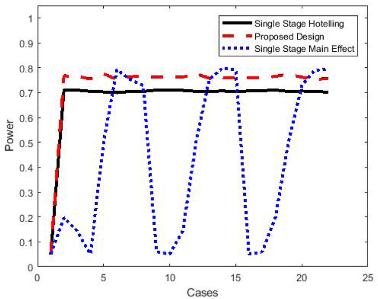
Comparison of power to reject the active factor null hypothesis for different tests given the parameter values described in Table 1. The black line and the blue line are for the single-stage Hotelling’s test and the main effect test, respectively. The red line is for the proposed test using a two-stage experiment with 40% data in first stage.
We further examine the robustness of the results in settings when the within-group variance is assumed to be unknown and when the within-group variances are unequal. The left plot in Figure 4 summarizes the power when all groups have equal within-group variance, but the within-group variance is assumed to be unknown. The right plot in Figure 4 summarizes the power when the data are generated with and the within-group variance is assumed to be unknown. We can see that the pattern of power comparison holds generally, with the proposed two-stage test having better power than the single-stage Hotelling’s test, and both are more robust than main effect testing.
Figure 4.

Comparison of power to reject the active factor null hypothesis for different tests under various parameter values: the black line and the blue line are for the single-stage Hotelling’s test and the main effect test, respectively. The red line is for the proposed test using a two-stage experiment with 40% data in the first stage. The figure on the left shows the case of unknown equal group variances, and the figure on the right shows the case of unknown and unequal group variances.
4. Illustrative Example
We describe a motivating example of a shoulder pain study. George et al. (2014) conducted a study to investigate genetic factors that interact with psychological factors on shoulder pain. A main focus was on the effect of the catechol-O-methyltransferase (COMT) gene and its interactions with pain catastrophizing. The study enrolled 190 subjects from University of Florida graduate and undergraduate classes, as well as from the surrounding community. At the baseline session, demographic and psychological data were collected from each subject. Also in this session, collection of DNA was done via buccal swab, and an exercise-induced pain protocol was completed. The main response variables were shoulder pain intensity (7-day average) reported on numerical rating scale and whether or not shoulder pain duration exceeded one week. COMT was represented by the 4 established COMT SNPs (rs6269, rs4633, rs4818, and rs4680) that affect pain sensitivity. Pain catastrophizing was assessed with the Pain Catastrophizing Scale (PCS), which is a 13-item measure to quantify pain catastrophizing characterized by magnification and rumination of pain beliefs.
Let A indicate the presence of the COMT gene, which is our potential active factor, and let B indicate the presence of high pain catastrophizing (PCS ≥ 5), which defines our subpopulations. We first consider the continuous response variable pain intensity (7-day average). From the data, the four group means are µ0 = 1.4, µA = 1.6, µB = 1.5, and µAB = 2.2 with pooled within-group variance σ2 = 1.1. Using these parameters, to design our two-stage experiment to achieve 80% power to detect the active factor (COMT gene), a total of 152 subjects are needed. Of these, 40% or 60 subjects (15 in each group) must be recruited in the first-stage trial. Then, based on the first-stage trial results, 92 subjects (46 per group) must be further recruited into the two groups that have the largest difference in the first stage (most likely the two groups with PCS ≥ 5). In contrast, for the single-stage balanced experiment using 152 subjects, the power of Hotelling’s test and the main effect test are 77% and 75%, respectively. To achieve 80% power for these two tests, the single-stage experiment would need 164 and 172 subjects, respectively.
We now consider the binary response variable of whether or not the pain duration exceeds one week. In the four groups, the proportions of subjects experiencing pain duration longer than one week are p0 = 18.4%, pA = 23.1%, pB = 22.5%, and pAB = 40.5%, respectively. To achieve 80% power of detecting the active COMT factor, our two-stage design requires 412 subjects in total, with 160 subjects (40 per group) in the first stage. In contrast, the single-stage Hotelling’s test and main effect test need 460 and 484 subjects, respectively, to achieve the same 80% power.
5. Discussions and Conclusions
This paper focuses on the detection of an active factor, where we define a factor as active if it has a non-zero effect in at least one subpopulation of interest. Active factor testing requires a smaller overall sample size than testing each subpopulation separately, and it is more robust than main effect testing when interactions are present. Thus, this strategy may be valuable for exploratory and pilot testing, especially when there may be significant heterogeneity in the factor effect. To implement active factor testing, we suggest an adaptive enrichment strategy using a two-stage play-the-winner design to test the active factor null hypothesis. Adaptive enrichment strategies utilize first-stage information to enhance the power of detection. We recommend using a noncentral chi-square test to conduct the second stage test and using a weighted Fisher’s combination of the p-values from each stage. The noncentral chi-square test uses preliminary estimates from the first stage to construct a more powerful test in the second stage.
While the play-the-winner second-stage design is similar to some current enrichment clinical trials for subpopulation analysis, generally, the literature proposes multiple testing of intervention effect for the overall population as well as all subpopulations while our active factor approach only tests one single composite hypothesis. Also, the literature focuses on one-sided hypothesis tests, while our proposed test is two-sided. The two-sided test is applicable in discovery trials searching for active factors without prior knowledge of the direction of the effect.
In contrast to the small amount of power loss reported in the literature (Bauer and Kohne, 1994; Banik et al., 1996), we found that both the Fisher’s and inverse normal combination methods resulted in a substantial loss of power for two-stage tests when compared to a one-stage test. Previous studies considered one-sided tests of a simple hypothesis, whereas we considered a two-sided composite hypothesis H0 of two parameters. As we observed that the weighted combinations performed better than their unweighted counter-parts, we recommend using a weighted Fisher’s combination of the p-values from each stage to minimize this power loss. To compensate for the loss of power due to combination, we propose a play-the-winner design with a non-central chi-square test in the second stage. This strategy can improve power beyond that of a single-stage test.
One limitation of this method is reduced interpretability of study results as compared to a design that tests the factor effect in each subpopulation as a separate hypothesis. Such an approach would require an overall larger sample size as only a subset of the sample contributes to testing each hypothesis. For this reason, the active factor approach should be recognized as a tool to screen for potential effects while requiring fewer resources. It may more readily detect weak signals, especially in settings where the effect varies by subpopulation. Active factor testing is designed for settings where subpopulations are well-defined and can be selected a priori. Thus, active factor testing may not work well when we do not have prior information on potential interactions.
We describe the active factor testing framework in a simple 2×2 setting, with a binary factor and a binary subpopulation covariate. This framework can be expanded to the setting of k > 2 subpopulations or with multiple subpopulation covariates (e.g. 2×2×2), by re-assigning the larger sample sizes to the subpopulations with larger treatment differences in the first stage. This may be useful in settings where it is undesirable to limit investigation to a single subpopulation covariate. However, assigning all second stage samples to the subpopulation with the largest treatment difference may not be the optimal solution for these more complicated settings. Finding the optimal second stage sample size assignments in this setting is more mathematically complex, and it is identified as an area of future research.
For adaptive subgroup analysis, researchers have studied many strategies such as optimal early stopping rules (for strong evidence of effect existence or strong indication of no effect) or adaptively changing the sample size (Cui et al., 1999) to ensure a certain level of conditional power after the interim analysis. These issues are worthy of future investigations under the framework of the active factor testing established here.
Acknowledgments
Funding
Drs. Ding and Wu were supported by an NIH/NIA grant (P30AG028740), which funded an exploratory study on adaptive multi-factor multi-stage clinical trial methods to accelerate efforts in identifying efficacious and effective interventions for preventing decline in physical function, loss of mobility and progression to disability among older adults. Drs. Dean and Wu were also supported by an NIH/NIAID grant (R01AI139761) to develop innovative study designs and analysis methods.
References
- Anderson TW (2003). An introduction to multivariate statistical analysis. Wiley-Interscience
- Banik N, Kohne K, and Bauer P (1996). On the power of fisher’s combination test for two stage sampling in the presence of nuisance parameters. Biometrical Journal, 38(1):25–37. [Google Scholar]
- Bauer P, Bretz F, Dragalin V, König F, and Wassmer G (2016). Twenty-five years of confirmatory adaptive designs: opportunities and pit-falls. Statistics in Medicine, 35(3):325–347. [DOI] [PMC free article] [PubMed] [Google Scholar]
- Bauer P and Kohne K (1994). Evaluation of experiments with adaptive interim analyses. Biometrics, 50(4):1029–1041. [PubMed] [Google Scholar]
- Brannath W, Posch M, and Bauer P (2002). Recursive combination tests. Journal of the American Statistical Association, 97(457):236–244. [Google Scholar]
- Cui L, Hung HMJ, and Wang S-J (1999). Modification of sample size in group sequential clinical trials. Biometrics, 55(3):853–857. [DOI] [PubMed] [Google Scholar]
- European Medicines Agency (2014). Guideline on the investigation of subgroups in confirmatory clinical trials EMA/CHMP/539146.
- F. Rosenberger W, (1999). Randomized play-the-winner clinical trials 20:328–42. [DOI] [PubMed] [Google Scholar]
- George SZ, Parr JJ, Wallace MR, Wu SS, Borsa PA, Dai Y, and Fillingim RB (2014). Biopsychosocial influence on exercise-induced injury: genetic and psychological combinations are predictive of shoulder pain phenotypes. The Journal of Pain, 15(1):68–80. [DOI] [PMC free article] [PubMed] [Google Scholar]
- Hu F, Zhang L-X, and He X (2009). Efficient randomized-adaptive designs. The Annals of Statistics, 37(5A):2543–2560. [Google Scholar]
- Jennison C and Turnbull B (1999). Group Sequential Methods with Applications to Clinical Trials. Chapman & Hall/CRC Interdisciplinary Statistics CRC Press. [Google Scholar]
- Mehrotra D, Guan Q, and Guo Z (2017). A powerful learn-and-confirm pharmacogenomics methodology for randomized clinical trials. Presentation at Joint Statistical Meetings at Baltimore, Maryland. [Google Scholar]
- Posch M, Maurer W, and Bretz F (2011). Type i error rate control in adaptive designs for confirmatory clinical trials with treatment selection at interim. Pharmaceutical Statistics, 10(2):96–104. [DOI] [PubMed] [Google Scholar]
- Rosenblum M, Qian T, Du Y, Qiu H, and Fisher A (2016). Multiple testing procedures for adaptive enrichment designs: combining group sequential and reallocation approaches. Biostatistics, 17(4):650–662. [DOI] [PubMed] [Google Scholar]
- Scharfstein DO, Tsiatis AA, and Robins JM (1997). Semiparametric efficiency and its implication on the design and analysis of group-sequential studies. Journal of the American Statistical Association, 92(440):1342–1350. [Google Scholar]
- Shun Z, Lan KKG, and Soo Y (2008). Interim treatment selection using the normal approximation approach in clinical trials. Statistics in Medicine, 27(4):597–618. [DOI] [PubMed] [Google Scholar]
- Simon N and Simon R (2013). Adaptive enrichment designs for clinical trials. Biostatistics, 14(4):613–625. [DOI] [PMC free article] [PubMed] [Google Scholar]
- U.S. Food and Drug Administration (2013). Guidance for industry: Enrichment strategies for clinical trials to support approval of human drugs and biological products Silver Spring, MD: FDA. [Google Scholar]
- Wang S-J, James Hung H, and O’Neill RT (2009). Adaptive patient enrichment designs in therapeutic trials. Biometrical Journal, 51(2):358–374. [DOI] [PubMed] [Google Scholar]
- Wang S-J, O’Neill RT, and Hung HMJ (2007). Approaches to evaluation of treatment effect in randomized clinical trials with genomic subset. Pharmaceutical Statistics, 6(3):227–244. [DOI] [PubMed] [Google Scholar]
- Wei LJ and Durham S (1978). The randomized play-the-winner rule in medical trials. Journal of the American Statistical Association, 73(364):840–843. [Google Scholar]
- Wu SS, Li H, and Casella G (2006). Tests with optimal average power in multivariate analysis. Statistica Sinica, 16(1):255–266. [Google Scholar]
- Wu SS, Tu Y-H, and He Y (2014). Testing for efficacy in adaptive clinical trials with enrichment. Statistics in medicine, 33(16):2736–2745. [DOI] [PMC free article] [PubMed] [Google Scholar]
- Zelen M (1969). Play the winner rule and the controlled clinical trial. Journal of the American Statistical Association, 64(325):131–146. [Google Scholar]