Accuracy of the Flow Velocity and Three-directional Velocity Profile Measured with Three-dimensional Cine Phase-contrast MR Imaging: Verification on Scanners from Different Manufacturers

Abstract

Purpose:

The accuracy of flow velocity and three-directional velocity components are important for the precise visualization of hemodynamics by 3D cine phase-contrast MRI (3D cine PC MRI, also referred to as 4D-flow). The aim of this study was to verify the accuracy of these measurements of prototype or commercially available 3D cine PC MRI obtained by three different manufactures’ MR scanners.

Methods:

The verification of the accuracy of flow velocity in 3D cine PC MRI was performed by circulating blood mimicking fluid through a straight-tube phantom in a slanting position, such that the three-directional velocity components were simultaneously measurable, using three 3T MR scanners from different manufacturers. The data obtained were processed by phase correction, and the velocity and three-directional velocity components in the center of the tube on the central cross section of a slab were calculated. The velocity profile in each three directions and the composite velocity profiles were compared with the calculated reference values, using the Hagen–Poiseuille equation. In addition, velocity profiles and the spatially time-averaged velocity perpendicular to the tube were compared with the theoretical values and measured values by a flowmeter, respectively.

Results:

An underestimation of the maximum velocity in the center of the tube and an overestimation of the velocity near the tube wall due to partial volume effects were observed in all three scanners. A roughening and flattening of profiles in the center of the tube were observed in one scanner, due, presumably, to the low signal-to-noise ratio. However, the spatially time-averaged velocities corresponded well with the measured values by the flowmeter in all three scanners.

Conclusion:

In this study, we have demonstrated that the accuracy of flow velocity and three-directional velocity components in 3D cine PC MRI was satisfactory in all three MR scanners.

Introduction

Cine phase-contrast MRI (cine PC MRI) is an imaging method that allows quantitative information regarding velocity to be obtained by applying bipolar velocity-encoding (VENC) gradients.¹ Bipolar gradients, which apply in sequence gradient magnetic fields with the opposite direction (but with equal magnitude), induce phase shifts of protons. The phase shifts of stationary protons occur as a function of time, while those of moving protons occur as a function of both velocity and time, and this difference in phase allows the calculation of velocity. In ordinary PC MRI, echo signals generated by applying VENC, VENC [+] signals, as well as VENC [−] signals (without VENC), are acquired. Magnitude images are generated from VENC [−] signals, which allows information about vascular morphology to be obtained. The VENC [−] signals and VENC [+] signals acquired after applying VENC in x, y, and z directions are processed to generate images with Fourier transform, and the phase images can be obtained by subtracting the former images from the latter images. The phase images acquired yield information concerning velocity in three directions.¹ Since 3D cine PC MRI (also referred to as 4D-flow) data concerning velocity in three directions is obtained three-dimensionally,² the 3D intravascular velocity field can be visualized as a vector diagram after processing the data using analytical software.^2–4

Hemodynamics such as wall shear stress (WSS) of a vascular wall and streamlines can be observed using 3D velocity fields acquired by 3D cine PC MRI.⁵ Several studies have reported that WSS is associated with the occurrence of, development of, and rupture of intracranial aneurysm.^6–8 Thus, there are important clinical applications for hemodynamic analysis using 3D cine PC MRI.

Since blood flow at any cross section of a vessel can be calculated using 3D cine PC MR images, the information acquired can be utilized as boundary conditions in the analysis of computational fluid dynamics.^4,9,10

For precise visualization of 3D velocity fields, the accuracy of velocities and three-directional velocity components are important. To the best of the authors’ knowledge, no studies have been reported that verify the accuracy of these parameters.

This aim of this study was to verify the accuracy of flow velocity and 3D velocity components of prototype or commercially available 3D cine PC MRI using three scanners (GE Healthcare [Milwaukee, WI, USA], Philips [Amsterdam, The Netherlands], and Siemens [Erlangen, Germany]) with a straight-tube phantom (inner diameter, 7 mm) positioned on a slant.

Materials and Methods

Phantom and flow passage

A phantom was purposely prepared for the verification of accuracy procedure using an acrylic straight tube (inner diameter, 7 mm; outer diameter, 16 mm). This was inserted into an acrylic 10-cm cube along the diagonal and fixed with 2 wt% agarose containing 0.0125 mmol/L Gd, a preparation designed to mimic the relaxation time of the cerebral white matter (Fig. 1).¹¹ A 40 wt% glycerin solution was used as a blood mimicking fluid. The viscosity was measured with a viscometer (VM-10A, CBC Materials, Tokyo, Japan) at 3.54 mPa·s. The flow passage consisted of a magnetic pump (CP20-PPRV-10, Nikkiso Eiko Co., Ltd., Tokyo, Japan), the phantom, a Coriolis flowmeter (FD-SF1, Keyence Corporation, Osaka, Japan), and a reservoir (Fig. 2). The distance between the phantom in the MR suite and the flowmeter placed in MR operation room was around 8 m. We used 15 mm-inner-diameter tube made of polyvinyl chloride with the pressure resistance of 0.8 MPa (SUPER TOYORON HOSE; TOYOX Co., Ltd., Kurobe, Japan) as main connecting tubes.

Fig. 1.

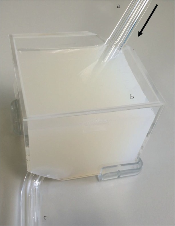
Phantom used in this study. (a) The tube near the inlet of the phantom (inner diameter, 7 mm; outer diameter, 16 mm), (b) agarose surrounding the phantom in an acrylic container (10 × 10 × 10 cm³), (c) the tube near the outlet. The arrow represents the flow direction.

Fig. 2.

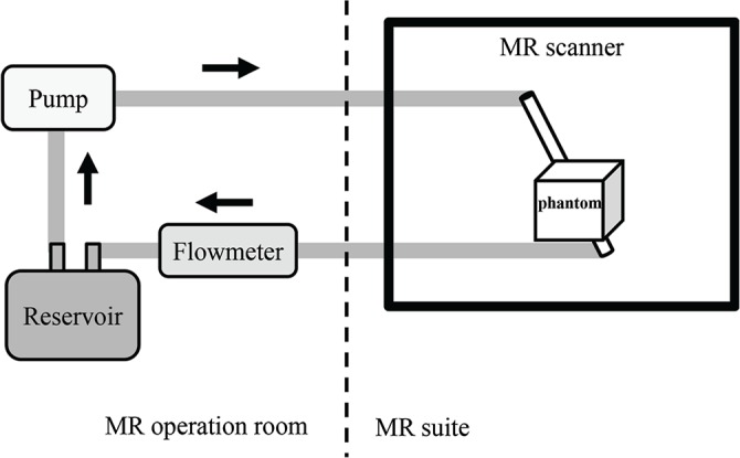
Flow channel used in the flow experiment. Arrows indicate the direction of the flowing fluid.

In order to obtain laminar flow with fully developed velocity profile, hydrodynamic entrance length is necessary. The entrance length can be obtained by the following formula:

$$L=0.05\times Re\times D{,}^{12}$$

where Re is Reynolds number (ρuD/μ), D is inner diameter, ρ is density, u is average velocity, μ is viscosity. The viscosity of human blood is about 4 mPa·s. The 40 wt% glycerin solution has this viscosity at 20°C, but the temperature in the MR suit and MR operation room was somewhat higher and the viscosity of the glycerin solution was 3.54 mPa·s. The hydrodynamic entrance length of the diagonal phantom permitted for MR gantry was 30 cm in this study. Based on the above conditions, the average velocity of working fluid should be set to 30 cm/s. The volume flow rate (VFR) was controlled by adjusting the voltage of the pump to achieve a steady circulation flow of the fluid set at a spatial-averaged velocity of 30 cm/s within the phantom. The fluctuation of the pump output volume during the imaging time was about 1%.

Scanners and imaging conditions

We used three MR scanners: Discovery 750w 3T, Head/neck coil (GE Healthcare); Ingenia 3T, dstream Head Spine coil (Philips); MAGNETOM Verio 3T, 12-channel Head Matrix coil (Siemens). The above-mentioned phantom was positioned inside a receiver coil. Axial, coronal, and sagittal images were acquired using simulated electrocardiogram-gating or triggering with the parameters shown in Table 1. The imaging sequence of Siemens was commercially unavailable, while others were manufactured. Three orthogonal VENC directions were set along phase encoding, frequency and slice encoding directions on each imaging orientation. We used the balanced (Hadamard) velocity encoding for 3D cine PC MRI using Philips equipment. Aliasing occurs at lower velocities than VENC we set.¹³ Therefore, we set VENC (120 cm/s) twice as large as the VENC of other equipment (60 cm/s). The reasons for the long imaging time of the Siemens equipment were that the simulated electrocardiographic interval was longer than that of the other experiments and it was impossible to use the imaging time reduction technology like view sharing technique. As Hadamard velocity encoding was used, the imaging time was shorter in Philips equipment.

Table 1.

Parameters of 3D cine phase-contrast MR imaging manufactured by GE Healthcare (Milwaukee, WI, USA), Philips (Amsterdam, The Netherlands), and Siemens (Erlangen, Germany)

Parameter	GE	Philips	Siemens
TR/TE (ms)	9.95/3.26	6.50/3.44	8.8/4.59
NEX	1	1	1
Flip angle (°)	15	10	15
FOV (mm)	180 × 180 × 36	180 × 180 × 35	190 × 190 × 35
Matrix	256 × 256 × 52	256 × 256 × 50	256 × 256 × 50
Voxel size (mm)	0.70 × 0.70 × 0.70	0.70 × 0.70 × 0.70	0.74 × 0.74 × 0.70
Bandwidth (Hz/pixel)	488	669	476
VENC (cm/s)	60	120	60
Parallel factor	ARC 2	SENSE 2	GRAPPA 2
ECG gating/triggering	Retrospective gating	Retrospective gating	Prospective triggering
Setting for the number of lines filled in k-space during one cardiac cycle	View per segment 4	TFE factor 4 phase 50%	Segment 4
No. of phases	4	4	4
R–R interval (ms)	500	500	700
Acquisition time	11 m 32 s	6 m 48 s	26 m 16 s

ARC, autocalibrating reconstruction for cartesian; ECG, electrocardiography; FA, flip angle; GRAPPA, generalized auto calibrating partially parallel acquisition; NEX, number of excitation; SENSE, sensitivity encoding; TFE, turbo field echo; VENC, velocity encoding.

We set a slab in the center of the phantom in axial, coronal or sagittal orientation. Magnitude images, phase images in the phase, readout and slice encoding directions, and velocity composite images of each section were obtained.

Post-processing

The temporal mean velocity profiles in the center of the tube on the central cross section of a slab were calculated from the 3D cine PC MR image data using the blood flow analyzing software (Flova, Renaissance of Technology Corporation, Hamamatsu, Japan). The phase correction protocol was performed using the surrounding agarose as a stationary phantom according to the method by Walker et al.¹⁴ The flow inside the tube of the phantom was considered to be laminar Hagen–Poiseuille flow¹⁵ because Reynolds number of the flow inside the tube was around 600 (lower than 2100). Therefore, measured velocity profiles inside the tube of the phantom were compared using the calculated parabolic profiles according to the VFR values measured with a flowmeter and the inner diameter of the tube as reference values. In order to remove noise derived from the acrylic tube, the velocity was set as 0 cm/s at the region where the standard deviation (SD) values were higher than 30. We also calculated velocity profiles and the spatially time-averaged flow velocity of the section perpendicular to the straight tube at the central part of the slab for each scanner.

A circular ROI with a diameter of 2 cm was selected at the position of the agarose surrounding the tube to measure the SD of pixel values for evaluation of the SD values of velocity in the stationary portion. ROI selection for this purpose required a region where the phase encoding direction did not overlap with the tube and where the fold-back in the slice orientation did not overlap. The following formulae were used as appropriate for each scanner for converting pixel values to velocity.

$$\text{GE}:\text{Velocity}=\frac{\text{Pixel}\hspace{0.17em}\text{value}\hspace{0.17em}\times \text{VENC}}{\text{Velocity}\hspace{0.17em}\text{encode}\hspace{0.17em}\text{scale}\times \pi }$$

$$\begin{array}{l}\text{Philips}:\hspace{0.17em}\text{Velocity}=\text{Pixel}\hspace{0.17em}\text{value}\times \text{Rescale}\hspace{0.17em}\text{slope}\\ \hspace{0.17em}\hspace{0.17em}\hspace{0.17em}\hspace{0.17em}\hspace{0.17em}\hspace{0.17em}\hspace{0.17em}\hspace{0.17em}\hspace{0.17em}\hspace{0.17em}\hspace{0.17em}\hspace{0.17em}\hspace{0.17em}\hspace{0.17em}\hspace{0.17em}\hspace{0.17em}\hspace{0.17em}\hspace{0.17em}\hspace{0.17em}\hspace{0.17em}\hspace{0.17em}\hspace{0.17em}\hspace{0.17em}\hspace{0.17em}\hspace{0.17em}\hspace{0.17em}\hspace{0.17em}\hspace{0.17em}\hspace{0.17em}\hspace{0.17em}\hspace{0.17em}\hspace{0.17em}\hspace{0.17em}\hspace{0.17em}\hspace{0.17em}\hspace{0.17em}\hspace{0.17em}\hspace{0.17em}\hspace{0.17em}\hspace{0.17em}\hspace{0.17em}\hspace{0.17em}+\text{Rescale}\hspace{0.17em}\text{intercept}\end{array}$$

$$\text{Siemens}:\hspace{0.17em}\text{Velocity}=\frac{\begin{array}{l}\text{Pixel}\hspace{0.17em}\text{value}\times \text{Rescale}\hspace{0.17em}\text{slope}\\ +\text{Rescale}\hspace{0.17em}\text{intercept}\end{array}}{4096}\times {\text{VENC}}_{}^{}$$

Results

Figure 3 shows the anatomical images and phase images in three directional encoding on axial orientation obtained by each vendor. The velocity profiles of the flow in a tube with an inner diameter of 7 mm obtained by 3D cine PC MRI demonstrated that maximum velocity was underestimated and velocity near the tube wall was overestimated in all scanners (Figs. 4 and 5). A roughening and flattening of velocity profiles in the center of the tube was observed in the scanner manufactured by Philips. However, the accuracy of three-directional velocity components was adequate in every scanner. The spatially time-averaged flow velocity of the section perpendicular to the straight tube at the central part of the slab for each scanner is shown in Table 2. They corresponded well with the measured values by the flowmeter in all three scanners.

Fig. 3.

The anatomical images and phase images in three directional encoding on axial orientation from 3D cine phase-contrast (PC) MR images obtained by the scanner manufactured by GE Healthcare (Milwaukee, WI, USA), Philips (Amsterdam, The Netherlands), and Siemens (Erlangen, Germany). The anatomic image of GE is a magnitude image, that of Phillips is a modulus image and that of Siemens is a rephrased image. Phase images obtained by Philips show the signal at the area with noise as zero with the use of noise clipping. Each velocity-encoding (VENC) direction of the phase images are frequency encode direction, phase encode direction and slice encode direction respectively on the axial orientation image. The polarity of the phase image varies with each device.

Fig. 4.

The velocity profiles of axial, coronal and sagittal sections from 3D cine phase-contrast (PC) MR images obtained by the scanner manufactured by GE, Philips and Siemens. The velocity profiles from 3D cine PC MR images obtained by GE (A), Philips (B) and Siemens (C) are shown. The velocity profiles of the phase encoding direction obtained by imaging in the axial (a), coronal (b), and sagittal (c) orientations. Similarly, (d–i) are velocity profiles of frequency encoding direction and slice encoding direction respectively. The composite velocity profiles in three directions obtained by imaging in the axial (j), coronal (k), and sagittal (l) orientations. The vertical axis in each graph represents the velocity and the horizontal axis represents the position inside the tube of the phantom. The broken line represents the reference values of the Hagen–Poiseuille flow. ♦ and the line represent analytic values.

Fig. 5.

The velocity profiles of sections perpendicular to the straight tube from 3D cine phase-contrast (PC). MR images obtained by the scanner manufactured by GE Healthcare (Milwaukee, WI, USA), Philips (Amsterdam, The Netherlands), and Siemens (Erlangen, Germany).

Table 2.

Spatially time-averaged velocity of the vertical section to the straight tube from 3D cine phase-contrast (PC) MR axial, coronal or sagittal orientation images obtained by the scanner manufactured by GE Healthcare (Milwaukee, WI, USA), Philips (Amsterdam, The Netherlands), and Siemens (Erlangen, Germany) and reference velocities obtained by the flowmeter

Flow measurement method		Vendors
		GE	Philips	Siemens
3D cine PC MRI	Axial orientation	29.2 ± 0.13	30.8 ± 0.18	31.5 ± 0.11
	Coronal orientation	28.8 ± 0.21	33.0 ± 0.25	29.4 ± 0.22
	Sagittal orientation	30.8 ± 0.09	30.6 ± 0.27	29.4 ± 0.08
Flowmeter		29.9 ± 0.23	29.5 ± 0.43	30.0 ± 0.38

Velocity value are represented as ‘average velocity ± SD’. Unit is cm/s.

The SD values of the velocity in the stationary portion in 3D cine PC MR images were 0.82–0.94 cm/s for GE, 2.27–2.86 cm/s for Philips, and 1.81–2.01 cm/s for Siemens (Table 3). No characteristic SD values for the velocity in the direction of the gradient magnetic field were observed in any of the scanners.

Table 3.

The SD values of the velocity in the stationary portion in the phase images acquired from 3D cine phase-contrast (PC) MR axial, coronal or sagittal orientation images obtained by the scanner manufactured by GE Healthcare (Milwaukee, WI, USA), Philips (Amsterdam, The Netherlands), and Siemens (Erlangen, Germany)

Vendors	Slice orientation	Velocity SD of phase encoding direction	Velocity SD of frequency encoding direction	Velocity SD of slice encoding direction
GE	Axial	0.85	0.82	0.80
	Coronal	0.89	0.94	0.90
	Sagittal	0.86	0.94	0.87
Philips	Axial	2.31	2.33	2.27
	Coronal	2.71	2.81	2.86
	Sagittal	2.81	2.73	2.67
Siemens	Axial	1.81	1.89	1.85
	Coronal	1.87	1.87	1.83
	Sagittal	2.00	2.01	1.97

Unit is cm/s SD, standard deviation.

Discussion

Performing 3D cine PC MRI using a phantom positioned at a slant enabled us to analyze three-directional velocity components in a single imaging. In addition, imaging in three orientations allowed for verification of the accuracy in each of the imaging conditions.

In the velocity profiles obtained by 3D cine PC MRI with each scanner, velocity near the tube wall was not 0 cm/s, and a positive flow was observed in all cases. The maximum velocity in the center of the tube was also underestimated. Partial volume effects may have caused these results. A roughening and flattening of velocity profiles in the center of the tube was observed in the scanner manufactured by Philips. Presumably, the signal-to-noise ratio (SNR) was too low under the imaging conditions used. Indeed, the Philips scanner demonstrated the largest SD values for the velocity calculated in the stationary portion. However, since the velocity profiles were satisfactory, except for those in the central portion of the tube, the accuracy of three-directional velocity components was adequate.

On the other hand, the spatially time-averaged flow velocity of the section perpendicular to the straight tube at the central part of the slab for each scanner corresponded well with the measured values by the Coriolis flowmeter in all three scanners.

There were two limitations to this study. First, because the parameter setting protocol was different in each scanner, the imaging parameters could not be unified. Second, due to the size and shape of the phantom including the 30-cm entrance region necessary for the formation of a laminar flow, the phantom could not be positioned in the exact center of the coil with different scanners leading to slight variations of position. Therefore, the imaging conditions may not have been optimal. Previously published paper reported that the error rate of the maximum velocity is less than 10% when the ratio of the pixel size to the inner diameter is less than 10%.¹⁶ In this experiment, the voxel size was 10% of the diameter (voxel size, 0.7 mm; diameter, 7 mm), but the error of the maximum velocities of some scanners exceeded 10%. It is estimated that the measurement error of the maximum flow velocity would be less than 10% if we had used optimum conditions including imaging parameters, receiver coil, imaging position, and so on.

Conclusion

Our study concerning the verification of the accuracy of flow velocity and three-directional velocity components by 3D cine PC MRI using scanners manufactured by GE, Philips, and Siemens with a straight-tube phantom positioned at a slant demonstrated that the accuracy achieved is satisfactory in every scanner. By setting the appropriate parameters and conditions, precise 3D velocity fields can be clearly visualized.

References

- 1.Pelc LR, Pelc NJ, Rayhill SC, et al. Arterial and venous blood flow: noninvasive quantitation with MR imaging. Radiology 1992; 185:809–812. [DOI] [PubMed] [Google Scholar]
- 2.Markl M, Chan FP, Alley MT, et al. Time-resolved three-dimensional phase-contrast MRI. J Magn Reson Imaging 2003; 17:499–506. [DOI] [PubMed] [Google Scholar]
- 3.Isoda H, Hirano M, Takeda H, et al. Visualization of hemodynamics in a silicon aneurysm model using time-resolved, 3D, phase-contrast MRI. AJNR Am J Neuroradiol 2006; 27:1119–1122. [PMC free article] [PubMed] [Google Scholar]
- 4.Isoda H, Ohkura Y, Kosugi T, et al. Comparison of hemodynamics of intracranial aneurysms between MR fluid dynamics using 3D cine phase-contrast MRI and MR-based computational fluid dynamics. Neuroradiology 2010; 52:913–920. [DOI] [PMC free article] [PubMed] [Google Scholar]
- 5.Isoda H, Ohkura Y, Kosugi T, et al. In vivo hemodynamic analysis of intracranial aneurysms obtained by magnetic resonance fluid dynamics (MRFD) based on time-resolved three-dimensional phase-contrast MRI. Neuroradiology 2010; 52:921–928. [DOI] [PubMed] [Google Scholar]
- 6.Meng H, Wang Z, Hoi Y, et al. Complex hemodynamics at the apex of an arterial bifurcation induces vascular remodeling resembling cerebral aneurysm initiation. Stroke 2007; 38:1924–1931. [DOI] [PMC free article] [PubMed] [Google Scholar]
- 7.Dolan JM, Kolega J, Meng H. High wall shear stress and spatial gradients in vascular pathology: a review. Ann Biomed Eng 2013; 41:1411–1427. [DOI] [PMC free article] [PubMed] [Google Scholar]
- 8.Meng H, Tutino VM, Xiang J, Siddiqui A. High WSS or low WSS? Complex interactions of hemodynamics with intracranial aneurysm initiation, growth, and rupture: toward a unifying hypothesis. AJNR Am J Neuroradiol 2014; 35:1254–1262. [DOI] [PMC free article] [PubMed] [Google Scholar]
- 9.Onishi Y, Aoki K, Amaya K, et al. Accurate determination of patient-specific boundary conditions in computational vascular hemodynamics using 3D cine phase-contrast MRI. Int J Numer Method Biomed Eng 2013; 29: 1089–1103. [DOI] [PubMed] [Google Scholar]
- 10.Isoda H, Takehara Y, Kosugi T, et al. MR-based computational fluid dynamics with patient-specific boundary conditions for the initiation of a sidewall aneurysm of a basilar artery. Magn Reson Med Sci 2015; 14:139–144. [DOI] [PubMed] [Google Scholar]
- 11.Fukuyama A, Mori M, Haba T, et al. A flow phantom to evaluate velocity encoding in three directions separately and verify the accuracy of flow velocity measurements. ECR 2015, Viena, 2015, ECR 2015 / C-0729. https://posterng.netkey.at/esr/viewing/index.php?module=viewing_poster&doi=10.1594/ecr2015/C-0729 (accessed April 23, 2018). [Google Scholar]
- 12.Incropera FP, Dewitt DP, Bergman TL, Lavine AS. Laminar flow in circular tubes: thermal analysis and convection correlations, In: Fundamentals of heat and mass transfer. Hoboken, NJ: John Wiley & Sons, Inc, 2007; 505–513. [Google Scholar]
- 13.Pelc NJ, Bernstein MA, Shimakawa A, Glover GH. Encoding strategies for three-direction phase-contrast MR imaging of flow. J Magn Reson Imaging 1991; 1:405–413. [DOI] [PubMed] [Google Scholar]
- 14.Walker PG, Cranney GB, Scheidegger MB, Waseleski G, Pohost GM, Yoganathan AP. Semiautomated method for noise reduction and background phase error correction in MR phase velocity data. J Magn Reson Imaging 1993; 3:521–530. [DOI] [PubMed] [Google Scholar]
- 15.Sutera SP, Skalak R. The history of Poiseuille’s law. Ann Rev Fluid Mechanics 1993; 25:1–20. [Google Scholar]
- 16.Fukuyama A, Isoda H, Morita K, et al. Influence of spatial resolution in three-dimensional cine phase contrast magnetic resonance imaging on the accuracy of hemodynamic analysis. Magn Reson Med Sci 2017; 16:311–316. [DOI] [PMC free article] [PubMed] [Google Scholar]