Improving Low-Dose Pediatric Abdominal CT by Using Convolutional Neural Networks

Abstract

Purpose

To evaluate the efficacy of convolutional neural networks (CNNs) to improve the image quality of low-dose pediatric abdominal CT images.

Materials and Methods

Images from 11 pediatric abdominal CT examinations acquired between June and July 2018 were reconstructed with filtered back projection (FBP) and an iterative reconstruction (IR) algorithm. A residual CNN was trained using the FBP image as the input and the difference between FBP and IR as the target such that the network was able to predict the residual image and simulate the IR. CNN-based postprocessing was applied to 20 low-dose pediatric image datasets acquired between December 2016 and December 2017 on a scanner limited to reconstructing FBP images. The FBP and CNN images were evaluated based on objective image noise and subjective image review by two pediatric radiologists. For each of five features, readers rated images on a five-point Likert scale and also indicated their preferred series. Readers also indicated their “overall preference” for CNN versus FBP. Preference and Likert scores were analyzed for individual and combined readers. Interreader agreement was assessed.

Results

The CT number remained unchanged between FBP and CNN images. Image noise was reduced by 31% for CNN images (P < .001). CNN was preferred for overall image quality for individual and combined readers. For combined Likert scores, at least one of the two score types (Likert or binary preference) indicated a significant favoring of CNN over FBP for low contrast, image noise, artifacts, and high contrast, whereas the reverse was true for spatial resolution.

Conclusion

FBP images can be improved in image space by a well-trained CNN, which may afford a reduction in dose or improvement in image quality on scanners limited to FBP reconstruction.

© RSNA, 2019

Summary

Convolutional neural networks can reduce image noise and artifacts to improve low-dose pediatric abdominal CT images reconstructed with filtered back projection.

Key Points

• ■ Well-trained convolutional neural network models can improve image quality for examinations acquired on CT scanners with filtered back projection reconstruction algorithms.

• ■ Applying convolutional neural network processing in the CT scanner or at the radiologist review station can increase the speed of iterative reconstruction and reduce the delay between acquisition and interpretation, which is particularly important in acute clinical settings, such as trauma.

Introduction

Concern over ionizing radiation dose resulting from CT examinations has led to a proliferation of research studies, new regulatory guidelines, and public awareness campaigns (1,2). The carcinogenic risk of ionizing radiation at levels used in diagnostic imaging (< 50 mSv) remains controversial, but minimizing cumulative exposure over a lifetime remains a central goal in pediatric imaging.

In an effort to reduce the amount of radiation required to produce a diagnostic image, CT scanner manufacturers have implemented iterative reconstruction (IR) algorithms, including image-based, model-based, and hybrid algorithms (3). Several limitations exist with regard to commercial IR. First, performing a full model-based IR is computationally intensive and time-consuming because the optimization of an objective function is performed in an iterative algorithm (3), and reconstruction time can approach 80 minutes (4) for some applications. As a result, manufacturers must strike a balance between accuracy and speed of reconstruction, typically opting for speed, given the potentially time-sensitive nature of CT, particularly in an emergency setting. The second limitation for reconstruction is that the CT scanner workstation is used for both data acquisition and image reconstruction. Although off-line reconstruction is possible, it is often not practical in a clinical setting, as it requires access to raw data and technical support, which is not easily granted by CT manufacturers. The image reconstruction is thus limited to the set of algorithms and convolution kernels on the scanner used for acquisition. The inherent coupling of acquisition and reconstruction restricts the available reconstruction options to the manufacturer, available computer hardware, and software version.

In this study, we leveraged a popular tool, deep learning, to decouple these steps, thereby allowing for optimization of each step independently. Applications of deep learning in radiology were recently summarized by Wang (5), and several deep learning techniques have been applied as a method of denoising low-dose CT images (6–9). Collecting data for network training is a challenge in CT as the low-dose and full-dose images must be synchronous (acquired at exactly the same time) in the same patient. Thus, even scanning the patient twice in quick succession is insufficient because of the time between acquisitions. Chen et al (9) inserted Poisson noise into images from the National Cancer Imaging Archive to develop a feature mapping tool from low- to normal-dose images. We pursued a tangential approach to develop a mapping tool between different reconstruction algorithms, namely the widespread filtered back projection (FBP) and IR.

We built off the approach of residual learning (10) to propose a residual network model to improve low-dose CT images, independent of scanner model and software (11). To this end, we have described a method of postprocessing FBP images in the standard Digital Imaging and Communications in Medicine (DICOM) format to simulate the appearance of a commercial IR algorithm with the expectation that, if successful, the method potentially can be applied to other IR algorithms if sufficient training data are available. By training a convolutional neural network (CNN) on a patient-matched FBP and IR image dataset, a simulated IR algorithm can be created and applied in image space to FBP images produced by any scanner. As a result, the scan and reconstruction steps can be decoupled, a step previously not possible because images were reconstructed from raw data in a proprietary format. This decoupling allows for examinations performed on a legacy CT scanner to be reconstructed with the image quality of state-of-the-art IR algorithms. In addition, it would allow a reconstruction algorithm from vendor A to be learned, simulated, and applied to data acquired on a scanner from vendor B. In this study, we evaluated the efficacy of applying CNNs to improve low-dose pediatric abdominal CT images in image space.

Materials and Methods

The institutional review board waived the informed consent requirement of this Health Insurance Portability and Accountability Act–compliant retrospective study.

Patient Demographics and CT Radiation Dose

The study consisted of a training dataset and review dataset. The training data consisted of 11 pediatric abdominal CT datasets acquired using a Siemens SOMATOM Force scanner (Siemens Healthineers, Forchheim, Germany) at Boston Children’s Hospital between June and July 2018. This scanner consists of two x-ray sources and detectors each with a 96 × 0.6–mm physical detector configuration for a total detector collimation of 192 × 0.6 mm, and patients were imaged with a pitch of 2.8. Each dataset was reconstructed at 5-mm image thickness with FBP (B31f kernel) and Siemens advanced modeled iterative reconstruction (ADMIRE) with a B31f kernel at strength 3 (ADMIRE-3). Example images used for training are shown in Figure 1. The datasets covered a wide range of patient ages (range, 1 month to 19 years; mean, 10.5 years) and radiation dose as quantified by the CT dose index with the 32 cm phantom (CTDI₃₂) (range, 0.4–15.0 mGy; mean, 3.11 mGy), size-specific dose estimate (range, 2.4–15.4 mGy; mean, 6.5 mGy), dose–length product (range, 7.22–862.9 mGy · cm; mean, 86.4 mGy · cm), and kilovolt peak (range, 70–150 kVp; median, 80 kVp). The size-specific dose estimate was calculated by using a water-equivalent diameter as described in the American Association of Physicists in Medicine Report 220 (12).

Figure 1a:

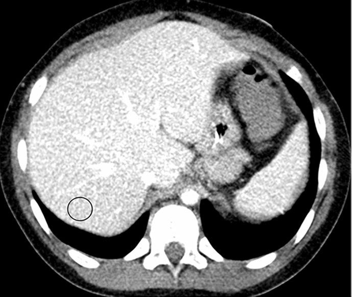
Example images used for training the convolutional neural network (window/level = 50/330 HU). (a, b) Abdominal CT images in a 9-year-old boy acquired with the institution’s dose class 2 protocol CT dose index: 1.57 mGy, 80 kV). Images are reconstructed in the (a) transaxial plane with Siemens weighted filtered back projection (FBP; kernel B31f) and (b) Siemens advanced modeled iterative reconstruction-3 (ADMIRE-3; kernel B31f/3). Hounsfield unit mean and noise power measured by HU standard deviation in the region of interest (circle) for FBP was 166.8 HU and 26.5 HU, respectively, and for ADMIRE-3 was 168.3 HU and 17.7 HU, respectively.

Figure 1b:

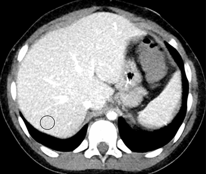
Example images used for training the convolutional neural network (window/level = 50/330 HU). (a, b) Abdominal CT images in a 9-year-old boy acquired with the institution’s dose class 2 protocol CT dose index: 1.57 mGy, 80 kV). Images are reconstructed in the (a) transaxial plane with Siemens weighted filtered back projection (FBP; kernel B31f) and (b) Siemens advanced modeled iterative reconstruction-3 (ADMIRE-3; kernel B31f/3). Hounsfield unit mean and noise power measured by HU standard deviation in the region of interest (circle) for FBP was 166.8 HU and 26.5 HU, respectively, and for ADMIRE-3 was 168.3 HU and 17.7 HU, respectively.

The review data included 20 patient datasets acquired by using a Siemens SOMATOM Sensation 40 scanner between December 2016 and December 2017. This scanner was capable only of FBP reconstruction, and images were reconstructed with a B31f kernel. As the review data were generated on a separate scanner from that used for the training data, no images used for review were included in the training set. This scanner consists of a single x-ray source and detector with a 20 × 0.6–mm physical detector configuration, and patients were imaged with a pitch of 1.3. Descriptive statistics for age and CT radiation dose of review data are as follows: patient age (range, 3–22 years; mean, 15.5 years), CTDI₃₂ (range, 1.0–6.9 mGy; mean, 2.5 mGy), size-specific dose estimate (range, 2.2–5.8 mGy; mean, 3.4 mGy), dose–length product (range, 30.1–247.7 mGy · cm²; mean, 100.5), and kilovolt peak (range, 100–120 kVp; median, 120 kVp). The imaging protocol was the hospital’s “dose class 3” (ie, lowest dose) abdomen protocol for indication of renal stones and was selected as these represented the noisiest images of the abdomen available in the hospital database. No oral or intravenous contrast material was administered. The higher kilovoltage was used because of the non–contrast material indication for renal stones.

CNN-based Image Mapping

The developed method consists of two phases: network training and image postprocessing. A diagram of the residual network is shown in Figure 2. In the training phase, the FBP-reconstructed image is used as the input of the network, and the residual between the FBP and ADMIRE-3 image is applied as the target. Hence, in the postprocessing phase, the well-trained network is able to predict the difference between the input FBP image and the expected ADMIRE-3 image. The simulated ADMIRE-3 image (here referred to as the CNN image) is then obtained by subtracting the generated residual noise pattern from the FBP image.

Figure 2:

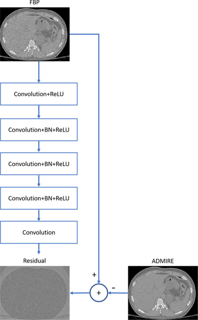
Schematic diagram shows the residual convolutional neural network (CNN) architecture used to train the network to simulate advanced modeled iterative reconstruction-3 (ADMIRE-3) in the CNN-processed image. There are five convolution layers, each with 32 kernels of size 3 × 3 pixels. Batch normalization (BN) is applied to correct the internal covariate shift after convolution, and a rectified linear unit (ReLU) is applied in the first four layers. The residual image between filtered back projection (FBP) and ADMIRE-3 inputs is applied at the target such that the well-trained network is able to predict the residual and remove it from the FBP, resulting in a CNN-processed image simulating the ADMIRE-3 reconstruction.

The input of the residual network is an FBP patch y, and the corresponding ADMIRE patch is x. We applied the residual learning formulation to train a residual mapping . Therefore, we have the estimated ADMIRE patch 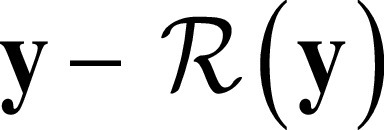. The loss function was defined as an averaged mean squared error between the desired residual patches and the estimated ones

where represents the trainable parameters in the CNN, denotes FBP-ADMIRE training patch pairs, where N is the number of patch pairs and is the Frobenius norm.

There are five convolutional layers in this network. Each layer consists of 32 convolutional kernels, and each is 3 × 3 in size. The stride is set to 1 pixel. Padding is performed to ensure that the size of the output image is the same as that of the input. In the second to fourth layers, batch normalization is used to solve the internal covariate shift after the convolution. Batch normalization introduces several advantages to the method, such as fast training and better performance (13). Finally, a rectified linear unit is applied to the first four layers as an activation function after the convolution or convolution plus batch normalization (14).

We adopted 11 patient samples to generate training data. Each sample has tens to hundreds of 512 × 512 images. We randomly extracted 64 × 64 small patches from those images, and 10 000 FBP-ADMIRE pair patches were generated. Then, these data were randomly split, and 90% of them were used for training and the remaining data were used for validation. The use of a large amount of training data can avoid overfitting during the training. The parameters of CNN were optimized using the Adam algorithm. The batch size was 16, and the learning rate was set to 0.01. The training completed after 200 epochs.

The CNN algorithm was based on the MatConvNet Matlab toolbox (15). The training was performed on a workstation with a Fx-6300 central processing unit (Advanced Micro Devices, Santa Clara, Calif) and an GeForce GTX 970 graphics processing unit card (NVIDIA, Santa Clara, Calif). The network training time was approximately 6 hours. After network training, image postprocessing was relatively fast, at approximately 50 images per minute.

CT Number and Image Noise

Image quality is evaluated with ground truth (ADMIRE images) and without ground truth. For the dataset with ground truth, the relative root-mean-square error was computed to quantitatively evaluate the noise reduction performance of the CNN processing. The relative root-mean-squared error is defined as:

where f represents the image to be evaluated and f_gt denotes the ground truth.

For the test dataset without ground truth, CT number and image noise power were measured for both the FBP and CNN datasets by recording the Hounsfield unit mean (HU_mean) and standard deviation (HU_sd) in a circular region of interest (area = 200 mm²) placed in the liver and spleen on the same image (when possible), as shown in Figure 3. Two patients were excluded owing to beam hardening and streaking artifacts from hardware that caused inaccuracies in the measured attenuation values.

Figure 3a:

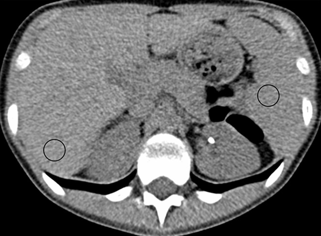
(a, b) Abdominal CT images (window/level = 50/330 HU) in a 16-year-old girl acquired with the institution’s dose class 3 protocol (CT dose index: 1.56 mGy, 120 kV). Images are reconstructed in the transaxial plane with (a) Siemens weighted filtered back projection (kernel B31f) and (b) convolutional neural network processing. Hounsfield unit mean and noise power measured by HU standard deviation in the region of interest (circle) for liver and spleen were as follows: liver, HU_mean = 62.5, HU_SD = 17.6; spleen: HU_mean = 51.3, HU_SD = 19.0 in a; and liver: HU_mean = 62.2, HU_SD = 11.5; spleen: HU_mean = 51.1, HU_SD = 12.6 in b.

Figure 3b:

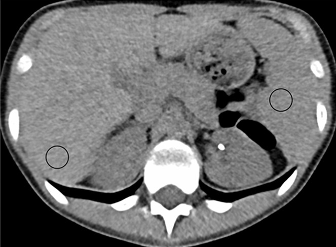
(a, b) Abdominal CT images (window/level = 50/330 HU) in a 16-year-old girl acquired with the institution’s dose class 3 protocol (CT dose index: 1.56 mGy, 120 kV). Images are reconstructed in the transaxial plane with (a) Siemens weighted filtered back projection (kernel B31f) and (b) convolutional neural network processing. Hounsfield unit mean and noise power measured by HU standard deviation in the region of interest (circle) for liver and spleen were as follows: liver, HU_mean = 62.5, HU_SD = 17.6; spleen: HU_mean = 51.3, HU_SD = 19.0 in a; and liver: HU_mean = 62.2, HU_SD = 11.5; spleen: HU_mean = 51.1, HU_SD = 12.6 in b.

Radiologist Review

FBP images from the review dataset were downloaded from the picture archiving and communications system (PACS) and then postprocessed with the CNN off-line to simulate the appearance of ADMIRE-3. Both the FBP- and CNN-processed series were pushed to a research PACS server.

Reviewers were asked to rate the images in the review dataset comprising 20 patients with two series per patient: the FBP series produced by the scanner and the CNN image series. The FBP and CNN series were assigned a random series number and order (1 or 2) such that the reviewers had no information if the series was FBP or CNN based on labels or ordering, and all overlay information was identical for both series. Images were reviewed on DICOM-calibrated radiologist reading monitors, and the reviewers were free to use all tools typically used for interpretation (pan, window and level, and zoom).

Two attending radiologists, reader 1 (J.P.R., 15 years of board-certification experience) and reader 2 (M.A.B., 3 years of experience), independently rated the following image features on a Likert scale, according to the following specified criteria: (a) spatial resolution, the ability to visualize the interface between the left kidney and spleen (1 = very unclear, 2 = unclear, 3 = neutral, 4 = clear, and 5 = very clear); (b) low contrast, the ability to identify a 1-cm low-attenuation lesion in the kidneys (1 = not confident, 2 = less confident, 3 = neutral, 4 = more confident, and 5 = very confident); (c) high contrast, the ability to identify a 1-mm (0.1 cm) stone in the kidneys (1 = not confident, 2 = less confident, 3 = neutral, 4 = more confident, and 5 = very confident); (d) image noise, the effect of image noise on the diagnosis of potential nephrolithiasis (1 = considerably impedes accurate diagnosis, 2 = slightly impedes accurate diagnosis, 3 = neutral, 4 = slightly helps accurate diagnosis, and 5 = considerably helps accurate diagnosis); and (e) artifacts, the severity of artifacts including beam hardening, streaking, and photon starvation (1 = many artifacts, 2 = some artifacts, 3 = neutral, 4 = slight artifacts, and 5 = few artifacts). In addition to scoring each feature on a Likert scale, reviewers also indicated a preferred series (or no preference) on the basis of each feature. They also indicated a preference on the basis of overall image quality.

Statistical Analysis

All statistical analyses outlined in this section were performed using SAS/STAT 14.1 software (SAS Institute, Cary, NC) (16). Specific SAS procedures used included FREQ (agreement and binary preference scores), IML (weighted agreement), TTEST (Likert scores), and GENMOD (combined reader versions of binary preference and Likert scores). All tests were at the 5% significance level.

Interreader agreement was assessed for CNN and FBP separately. For binary preferences, interreader agreement was measured by the proportion of agreement and κ (17). For Likert scores, agreement was measured by weighted versions of the proportion of agreement and κ, by using weights based on the squared error metric. We follow the Fleiss suggestion for interpreting magnitudes of agreement κ (18) (or weighted κ): values in ranges 0–0.40, 0.40–0.75, and 0.75–1 represent low, moderate, and high agreement, respectively. For the proportion (or weighted proportion) of agreement, these translate to the following: values in ranges 0–0.70, 0.70–0.875, and 0.875–1 represent low, moderate, and high agreement, respectively.

For HU_sd scores, means for CNN and FBP were tested for equality by using paired t tests, and 95% confidence intervals for the true differences were calculated. For HU_mean scores, means for CNN and FBP were tested for equivalence using two one-sided paired t tests, and 90% confidence intervals for the true differences were calculated (19). CNN was defined to be equivalent to FBP if the true mean for CNN (C) was within 1% of the true mean for FBP (F), that is, if C was in the equivalence interval (−0.01 F, 0.01 F). Significance of the equivalence test at the 5% level corresponds to the 90% confidence interval being entirely contained within this equivalence interval.

For each feature, Likert score means for CNN and FBP were tested for equality using paired t tests, and 95% confidence intervals for the true differences were calculated. The same method was applied to the overall average of the five feature scores, an outcome analogous to the overall binary preference score.

For each feature, and for overall preference, the proportion of image pairs in which CNN was preferred (score = 1) was compared with the proportion of image pairs in which FBP was preferred (score = 0). Responses indicating no preference were excluded from the analysis. An exact binomial test of H0 (P = .5) versus HA (P ≠ 0.5) was calculated, along with a 95% confidence interval. A Bayesian interval with a Jeffreys prior was used to accommodate skewness in the data.

For both preference and Likert scores, analyses using scores for both readers combined were based on a correlated marginal model estimated by generalized estimating equations (20). These models, which accommodate between-reader and between-method correlations, provide a single result using all the sample data.

Results

Objective Image Quality

Figure 4 shows the images reconstructed by FBP, ADMIRE, and CNN processing, where the ADMIRE image can be assumed as the reference (ground truth). The CNN-processed image has a lower noise level than that of FBP and is close to that of ADMIRE. The relative root-mean-square error of FBP is 8.21 × 10^-3, and this value is reduced to 4.92 × 10^-3 after CNN processing.

Figure 4a:

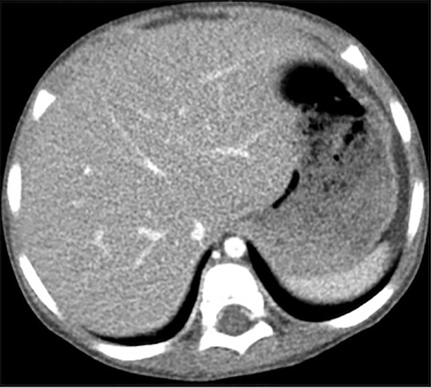
(a–c) Abdominal CT images in a 3-year-old girl acquired with the institution’s dose class 2 protocol (CT dose index: 0.50 mGy, 70 kV). Images are reconstructed in the transaxial plane with (a) Siemens weighted filtered back projection (kernel Br44d), (b) advanced modeled iterative reconstruction (kernel Br44d\3), and (c) convolutional neural network processing.

Figure 4b:

(a–c) Abdominal CT images in a 3-year-old girl acquired with the institution’s dose class 2 protocol (CT dose index: 0.50 mGy, 70 kV). Images are reconstructed in the transaxial plane with (a) Siemens weighted filtered back projection (kernel Br44d), (b) advanced modeled iterative reconstruction (kernel Br44d\3), and (c) convolutional neural network processing.

Figure 4c:

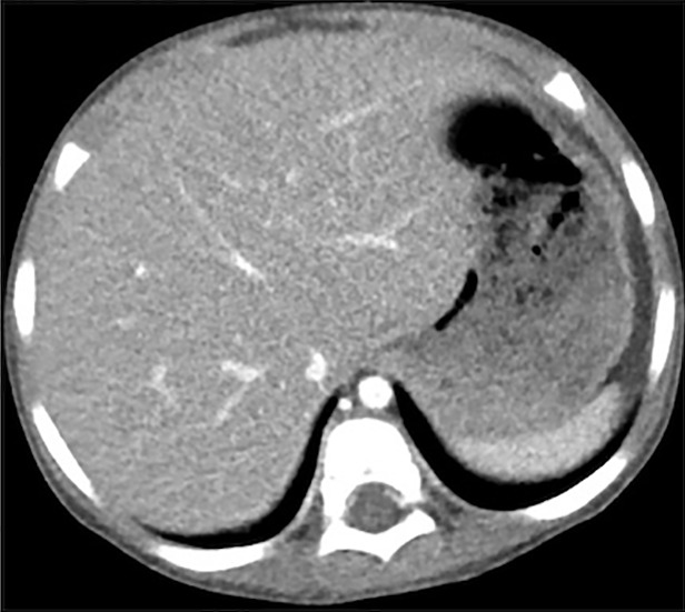
(a–c) Abdominal CT images in a 3-year-old girl acquired with the institution’s dose class 2 protocol (CT dose index: 0.50 mGy, 70 kV). Images are reconstructed in the transaxial plane with (a) Siemens weighted filtered back projection (kernel Br44d), (b) advanced modeled iterative reconstruction (kernel Br44d\3), and (c) convolutional neural network processing.

As shown in Table 1, means for HU_mean scores of CNN and FBP images were equivalent for both liver (P < .001) and spleen (P = .007), indicating that the population mean for CNN is within 1% of the population mean for FBP. Image noise, quantified by HU_sd, was significantly lower for CNN compared with that of FBP for both the liver (P < .001) and spleen (P < .001). The reduction in mean HU_sd scores was 6.8 (31%) and 7.0 (30%) for the liver and spleen, respectively, as shown in Figure 5.

Table 1:

Results of Objective Image Quality Analysis: Mean Attenuation in the Liver and Spleen

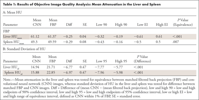
Figure 5:

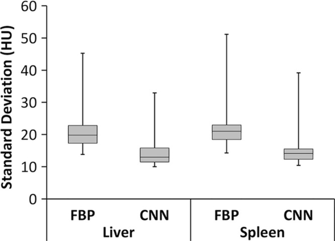
Box plot of standard deviation of HU in the liver and spleen for filtered back projection (FBP) and convolutional neural network (CNN) reconstruction for 18 image datasets. Box plots are formatted to show (from bottom to top) minimum, first quartile, median, third quartile, and maximum values.

Subjective Image Quality

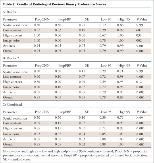
On the basis of binary preference scores (Table 2), when both readers were combined, there was a preference for CNN (ie, the proportion of image pairs in which CNN was preferred was > 0.50) for low contrast (0.85, P < .001), high contrast (0.85, P < .001), image noise (0.93, P < .001), artifacts (0.95, P < .001), and overall (0.95, P < .001). For reader 1, preferences were significant for high contrast (P = .031), image noise (P = .002), artifacts (P < .001), and overall (P < .001). For reader 2, preferences were significant for low contrast (P < .001), high contrast (P = .012), image noise (P < .001), artifacts (P < .001), and overall (P < .001).

Table 2:

Results of Radiologist Review: Binary Preference Scores

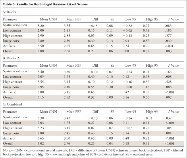
Likert scores (Table 3), when both readers were combined, indicated a preference for CNN for low contrast (0.27, P < .001), image noise (0.43, P = .004), artifacts (0.65, P < .001), and overall (0.26, P < .001). For reader 1, CNN scored higher for image noise (P = .030), artifacts (P < .001), and overall (P = .003). For reader 2, CNN scored higher for low contrast (P = .008), artifacts (P < .001), and overall (P = .002). For spatial resolution, FBP scored higher when both readers were combined (−0.13, P = .037), although this difference was not statistically significant for either reader individually (P = .083 for reader 1 and P = .163 for reader 2).

Table 3:

Results for Radiologist Review: Likert Scores

Interreader Agreement

Overall, agreement between the two readers was moderate to high when based on the proportion of agreement. For binary preference scores, the proportion of agreement ranged from 0.50 to 0.86 for individual features and was 0.86 (moderate) for overall preference. Agreement based on κ ranged from 0 to 0.25 for individual features and was 0.17 (low) for overall preference.

For Likert scores, the proportion of weighted agreement for CNN ranged from 0.89 to 0.92 for individual features and was 0.90 (high) for the overall score. For FBP, the corresponding proportions ranged from 0.88 to 0.93 for individual features and 0.90 (high) for the overall score. Agreement based on weighted κ for CNN ranged from 0.09 to 0.71 for individual features and was 0.31 (low) for the average score. For FBP, the corresponding proportions ranged from −0.09 to 0.73 for individual features and 0.24 (low) for the overall score.

Discussion

The results of objective image quality demonstrate that applying the CNN postprocessing in image space maintains CT number fidelity, an important requirement for any image processing or reconstruction algorithm. The basis of postprocessing is simply the subtraction of a predicted noise image, as this simplifies network training and does not shift the mean tissue value. The reduction in noise (HU_sd) is similarly intuitive, given the subtraction of the residual noise pattern. One limitation of this analysis was that HU_sd measures noise magnitude (the area under the noise power spectrum) and does not characterize noise texture. Noise power spectrum was not measured owing to nonlinearities in both the ADMIRE reconstruction and CNN-processed images, which preclude a linear system analysis.

On the basis of combined reader results, at least one of the two score types (Likert or binary preference) indicated a significant favoring of CNN over FBP for low contrast, image noise, artifacts, and high contrast, whereas the reverse was true for spatial resolution. Likert and binary preference scores were never contradictory (one significantly favoring one method and the other significantly favoring the other method), although the two score types did not always agree on the basis of conventional claims of statistical significance (P < .05 vs P ≥ .05). For high contrast, preference scores favored CNN (P < .001) but Likert scores did not (P = .305). For spatial resolution, Likert scores favored FBP (P = .037) but preference scores did not (P > .99). Possible explanations for the partial ambiguity of the two score types could be as follows. For high contrast, although CNN was preferred (binary score), this preference was in a wider sense than that allowed by the Likert scale. For spatial resolution, although a difference could be detected (Likert score), it was not considered important (binary score).

The results of spatial resolution might be explained in light of previous studies indicating a higher resolution for FBP versus ADMIRE-3 for low-dose levels and a shift in the noise power spectrum for various IR algorithms, potentially resulting in a smooth or plastic appearance perceived as a loss in spatial resolution for ADMIRE-3 (21,22). It is also possible that CNN postprocessing contributed slightly to a loss in resolution in addition to ADMIRE-3 and is a question we plan to investigate in the future. Similarly, with regard to high contrast, detection of a renal stone is not an overly demanding task, even with a relatively noisy background. Thus, it is reasonable that both FBP and CNN could have comparable performance for Likert scores for both of these features.

Both readers overwhelmingly preferred CNN for overall image quality preference. At least two interpretations are possible. First, given a choice, both readers prefer to interpret the CNN series with its perception of decreased image noise (even if there were no differences in diagnostic accuracy). Alternatively, there could be other features, which we did not test explicitly, but which are important in the context of the overall interpretation and better visualized on the CNN images. These contextual elements would not be scored with regard to our tested features but would affect overall preference.

There were several limitations to our study. First, we chose a single IR algorithm and kernel, Siemens ADMIRE-3 (B31f), to study so as to create a manageable database for radiologist review. Although the process of building a well-trained network uses open-source deep learning libraries, a separate network must be trained for each reconstruction to be applied to the FBP images, although future training could be accelerated with transfer learning techniques. Although not performed in this study, the training of many networks representing different IR algorithms and kernels (ie, image “looks”) presents the potential to produce custom, hybrid kernels that can be applied at the radiologist’s workstation at the time of review, eliminating the need for radiologist-preferred reconstructions to be programmed at the scanner. Our strategy can thus be adapted to apply a reconstruction algorithm from scanner A to data acquired on scanner B. This is possible as all processing is performed in image space. X-ray dose and reconstruction kernels are dominant factors for image quality, whereas the difference among different scanners (eg, size of detector bin and projection views per rotation) can be ignored. Thus, the trained network can be applied to other scanners, as long as the key acquisition parameters of test data are covered by the range of those in training data. Finally, although we have shown that conventional FBP images can be improved with CNN postprocessing, we have not attempted to show equivalence to existing IR algorithms. The reason for this is that the FBP images were sent from a scanner that did not have an IR option. For this reason, we chose to highlight the application of simulating IR to older legacy scanners as opposed to showing equivalence between CNN and commercial IR (eg, Siemens ADMIRE).

There are several important implications that follow from the success of our approach. First, the ability to decouple the acquisition and reconstruction steps could allow for arbitrary IR algorithms to be learned by standard CNN techniques and applied to FBP images produced by any scanner, resulting in a vendor-agnostic approach to CT image processing. Second, model-based IR algorithms, currently limited by computing time and hardware, could potentially be transferred to image space and applied to FBP images in a matter of seconds, obviating computer clusters at the CT scanner.

References

- 1.Strauss KJ, Goske MJ, Kaste SC, et al. Image gently: ten steps you can take to optimize image quality and lower CT dose for pediatric patients. AJR Am J Roentgenol 2010;194(4):868–873. [DOI] [PubMed] [Google Scholar]
- 2.Brink JA, Amis ES Jr. Image Wisely: a campaign to increase awareness about adult radiation protection. Radiology 2010;257(3):601–602. [DOI] [PubMed] [Google Scholar]
- 3.Zhang H, Wang J, Zeng D, Tao X, Ma J. Regularization strategies in statistical image reconstruction of low-dose x-ray CT: a review. Med Phys 2018;45(10):e886–e907. [DOI] [PMC free article] [PubMed] [Google Scholar]
- 4.Li G, Liu X, Dodge CT, Jensen CT, Rong XJ. A noise power spectrum study of a new model-based iterative reconstruction system: Veo 3.0. J Appl Clin Med Phys 2016;17(5):428–439. [DOI] [PMC free article] [PubMed] [Google Scholar]
- 5.Wang G. A perspective on deep imaging. IEEE Access 2016;4:8914–8924. [Google Scholar]
- 6.Kang E, Min J, Ye JC. A deep convolutional neural network using directional wavelets for low-dose x-ray CT reconstruction. Med Phys 2017;44(10):e360–e375. [DOI] [PubMed] [Google Scholar]
- 7.Yi X, Babyn P. Sharpness-aware low-dose CT denoising using conditional generative adversarial network. J Digit Imaging 2018;31(5):655–669. [DOI] [PMC free article] [PubMed] [Google Scholar]
- 8.Yang W, et al. Improving low-dose CT image using residual convolutional network. IEEE Access 2017;5:24698–24705. [Google Scholar]
- 9.Chen H, Zhang Y, Zhang W, et al. Low-dose CT via convolutional neural network. Biomed Opt Express 2017;8(2):679–694. [DOI] [PMC free article] [PubMed] [Google Scholar]
- 10.Zhang K, Zuo W, Chen Y, Meng D, Zhang L. Beyond a gaussian denoiser: residual learning of deep CNN for image denoising. IEEE Trans Image Process 2017;26(7):3142–3155. [DOI] [PubMed] [Google Scholar]
- 11.Zhang Y, MacDougall RD, Yu H. Convolutional neural network based CT image post-processing from FBP to ADMIRE. In: Fifth International Conference on Image Formation in X-Ray Computed Tomography, Salt Lake City, Utah: 2018; 411–414. [Google Scholar]
- 12.Larson DB, Malarik RJ, Hall SM, Podberesky DJ. System for verifiable CT radiation dose optimization based on image quality: Part II—Process control system. Radiology 2013;269(1):177–185. [DOI] [PubMed] [Google Scholar]
- 13.Ioffe S, Szegedy C. Batch normalization: accelerating deep network training by reducing internal covariate shift. arXiv:1502.03167v3. [preprint] https://arxiv.org/abs/1502.03167. Posted 2015. Accessed July 1, 2018.
- 14.Dahl GE, Sainath TN, Hinton GE. Improving deep neural networks for LVCSR using rectified linear units and dropout. In: 2013 IEEE International Conference on Acoustics, Speech, and Signal Process, Vancouver, BC, Canada. IEEE, 2013; 8609–8613. [Google Scholar]
- 15.Vedaldi A, Lenc K. MatConvNet: convolutional neural networks for MATLAB. arXiv:1412.4564v3. [preprint] https://arxiv.org/abs/1412.4564. Posted 2014. Accessed July 1, 2018.
- 16.SAS Institute . SAS/STAT 14.1 user guide. Cary, NC: SAS Institute, 2015. [Google Scholar]
- 17.Agresti A. Categorical data analysis. 3rd ed. Hoboken, NJ: Wiley, 2013. [Google Scholar]
- 18.Fleiss JL. Statistical methods for rates and proportions. 2nd ed. New York, NY: Wiley, 1981. [Google Scholar]
- 19.Wellek S. Testing statistical hypotheses of equivalence and noninferiority. New York, NY: Chapman and Hall/CRC, 2010. [Google Scholar]
- 20.Fitzmaurice GM, Laird NM, Ware JH. Applied longitudinal analysis. 2nd ed. Hoboken, NJ: Wiley, 2011. [Google Scholar]
- 21.Solomon J, Wilson J, Samei E. Characteristic image quality of a third generation dual-source MDCT scanner: noise, resolution, and detectability. Med Phys 2015;42(8):4941–4953. [DOI] [PubMed] [Google Scholar]
- 22.Mileto A, Zamora DA, Alessio AM, et al. CT detectability of small low-contrast hypoattenuating focal lesions: iterative reconstructions versus filtered back projection. Radiology 2018;289(2):443–454. [DOI] [PubMed] [Google Scholar]