Accurate segmentation of brain images into 34 structures combining a non-stationary adaptive statistical atlas and a multi-atlas with applications to Alzheimer’s disease

Abstract

Accurate segmentation of the 30+ subcortical structures in MR images of whole diseased brains is challenging due to inter-subject variability and complex geometry of brain anatomy. However a clinically viable solution yielding precise segmentation of the structures would enable: 1) accurate, objective measurement of structure volumes many of which are associated with diseases such as Alzheimer’s, 2) therapy monitoring and 3) drug development. Our contributions are two-fold. First we construct an extended adaptive statistical atlas method (EASA) to use a non-stationary relaxation factor rather than a global one. This permits finer control over adaptivity allowing 34 structures to be simultaneously segmented rather than just 4 as in [13]. Second we use the output of a weighted majority voting (WMV) label fusion multi-atlas method as the input to EASA in a hybrid WMV-EASA approach. We assess our proposed approaches on 18 healthy subjects in the public IBSR database and on 9 subjects with Alzheimer’s disease in the AIBL database. EASA is shown to produce state-of-the-art accuracy on healthy brains in a fraction of the time of comparable methods, while our hybrid WMV-EASA visibly improves segmentation accuracy for structures throughout the diseased brains.

1. INTRODUCTION

Accurate segmentation of magnetic resonance (MR) brain images, especially for whole diseased brains, is a fundamental yet challenging task because different anatomical structures may have similar intensity values. Manual segmentation has been shown to be sufficiently robust and accurate, but it is difficult and labor intensive. Therefore it is necessary to develop an automated and accurate algorithm to segment whole diseased brains.

There are several methods proposed to segment the brain into different anatomical structures using one or more atlases [1, 3, 6, 10, 13, 14, 16], or deformable models [8, 17]. The atlas based approaches can be grouped into two categories: single-atlas [1, 14] and multi-atlas [6, 10, 16] approaches. The single atlas approach constructs a statistical atlas from a set of training atlases from different subjects to model the spatial variability and appearance of brain structures. These atlas-based methods were shown robust and accurate since they can model different structures with similar intensity values. Statistical atlas methods are fast to segment the target, however can have lower accuracy when the target image has significant anatomical variation from the atlas population. To avoid such limitation, the multi-atlas methods register a set of atlases to the target scan, and then compute the final segmentation through a label fusion approach, e.g., majority voting [10]. Drawbacks can include high computation burden due to registration of several atlases, and the inability to handle diseased brains, not included among the set of atlases.

Recently, Shiee et al. [13] proposed a method with an adaptive atlas to deal with the limitation of single-atlas methods. Cardoso et al. [3] used a locally adaptive method to measure the cortical thickness. Their results are very promising; however, they only segment the brain into 4–6 basic structures such as white matter (WM), gray matter (GM), ventricles, CSF, etc. while many finer structures, such as the subcortical GM structures, which are critical in clinical diagnoses (e.g. hippocamups volumetry for Alzheimer’s) are not handled.

In this work, we propose two brain segmentation methods. The first is for healthy brains, which we call the extended adaptive statistical atlas (EASA), segments 34 structures throughout the whole brain at the high accuracy of the much slower multi-atlas methods but requiring just a few minutes per subject. The second method, WMV-EASA, is hybrid approach combining a multi-atlas (WMV) and EASA. It accurately segments the 34 structures even in severely diseased brains. We evaluate our methods extensively on two data sets with normal brains and diseased brains respectively.

2. METHODOLOGY

In this section we describe our two brain segmentation methods. For the first, EASA, an extension of [13] our primary contribution is the construction of a 3D non-stationary relaxation map from a fixed set of training data that spatially regulates atlas adaptivity voxel by voxel based on voxel label uncertainty. For the second, WMV-EASA we present a novel hybridization of a multi-atlas and statistical atlas methods and computation of a test subject tailored relaxation map.

Background: Adaptive statistical atlas.

In [13] Shiee et al. present a method which allows a statistical atlas to relax to enable the atlas, trained on a given limited set of brains (e.g. healthy), to segment brains not represented in the training set (e.g. diseased). It combines a Gaussian Mixture Model (GMM) and a Markov Random Field (MRF) [14] into an EM based approach. A key contribution was their use of a Dirichlet prior on the GMM mixing coefficients to guide the segmentation. This method assumes the brain consists of K structures (k = 1,…, K), the number of voxels in the MR image is N (i = 1,…, N), and the observed image can be modeled by a K-component GMM [14]. The true label for voxel i is denoted as z_i (a K × 1 binary-value vector), the prior probability that voxel i belongs to structure k as P_i = (p_i1,…, P_iK), and posterior probability as w_ik. In the EM framework the mixing coefficients are updated by a linear combination of p_ik and w_ik. The p_ik is allowed to relax to obtain a subject-specific atlas to segment a diseased scan from a normal atlas. This method uses a spatially invariant (globally constant) relaxation factor (adaptivity) k = 0.5 to control the amount of relaxation over the whole volumetric atlas. This was shown sufficient to enable the atlas to adapt and segment a novel brain into 3 or 4 basic structures (WM, GM and CSF). Since the brain is complex, it is desirable to segment many more structures including 30+ subcortical structures. A naive approach, denoted Naïve, would be to retain the same spatially invariant k and simply compute the spatial priors p_i for each additional structure. However, this leads to low segmentation accuracy. In the following section we present our first contribution, an extension which allows to adapt the atlas to segment 34 different structures in novel brains.

Extended adaptive statistical atlas method (EASA).

We spatially regulate relaxation in order to balance its positive and negative aspects. On the one hand it allows an atlas to segment brains not well represented in the training data. On the other hand it can allow too much adaptation of the atlas causing a structure to leak if similar enough intensities are found in neighboring structures. Based on this observation, we propose an extended adaptive statistical atlas method, EASA, whose relaxation map is spatially varied to adapt the statistical atlas to the target image in a principled fashion. We denote the coordinates of each voxel as $\text{x}\in {ℝ}^3.$ Our non-stationary relaxation map $\kappa (X):{ℝ}^3\mapsto ℝ)$ is built from the training data. First, we carefully non-linearly register [2] the training scans to a reference training scan, and propagate the labels from all subjects to the reference. Then we compute the label entropy at each voxel: $H(\text{x})={\sum }_{k=1}^K-r_k(\text{x})\log \left(r_k(\text{x})\right),$ where r_k (x) is the number of times that voxel is labeled as k divided by the number of scans in training data set. Since larger entropy means larger uncertainty, we allow larger relaxation at that voxel, and less where uncertainty is lower. We use a sigmoidal smooth transfer function to compute the relaxation map:

$$\kappa (x)=\frac{u-l}{1+exp(-E(x))}+l$$

where E(x) = M(H(x) – (S · min(H(x)) + (1 – S). max(H(x)))). M ≥ 1 scales the values, while $S\in (0,1)$ moves the inflection point of the sigmoid curve. Fig. 1 shows an example where M = 3.0, S = 0.1, l = 0.0, u = 0.5, and 0 ≤ H (x) ≤ 20. Note that k(x) = 0 allows only minimal relaxation while k(x) = 0.5 allows substantial relaxation.

Fig. 1:

Conversion of label entropy to relaxation map, k(x)

We set these parameters of the transfer function such that relaxation is much less near the center of larger structures and higher along the boundary. We denote the voxels in the region of structure k as $X_k=\left\{x|r_k(\text{x})>0\right\}.$ To construct the overall k(x) we apply the mapping function on every structure individually to compute ${\kappa }_k(\mathrm{x})=\left\{\kappa (\mathrm{x})|\mathrm{x}\in X_k\right\}.$ Then we compute $\kappa (\mathrm{X})=\frac{{\sum }_{k=1}^K{\kappa }_k(\mathrm{X})}{n(\mathrm{X})}$ where n(x) is the number of times that x is contained in X_k.

Next we construct the structure spatial priors p_ik from the co-registered training set. Construction of p_ik and k(x) are off-line procedures. For each test subject, EASA then performs two online steps: 1) roughly nonlinearly register [11] the intensity image from the reference training subject to target subject, and apply the same transformation on the p_ik and k(x); 2) initialize $w_{ik}^0$ by the transformed p_ik and then apply adaptive segmentation.

Background: Weighted Majority Voting (WMV).

In contrast to single statistical atlas methods (e.g. [13]), multiatlas methods register several training subjects to the test image and then choose the label for each voxel through a process called label fusion. Conventional majority voting label fusion determines the labels solely based on the atlas labels without considering the test intensity image. This can mislabel voxels at structure boundaries. To improve performance, the weighted majority voting method (WMV) [10] was developed which incorporates the test image intensity into conventional majority voting. WMV is formulated as: $\widehat{L}(\mathrm{x})=\arg {\max }_{l}p\left(L(\mathrm{x})=l|{\left\{L_n(\mathrm{x})\right\}}_1^N\right)p(I(\mathrm{x})|L(\mathrm{x})=l)$ where ${\left\{L_n(\mathrm{x})\right\}}_1^N$ are the labels at x from the N atlases, I(x) is test image intensity, and $\widehat{L}(\text{x})$ the fused label. p(I(x)|L(x) = l) ~ N (μl,σl) is the intensity distribution for label l in the test image. For a given label map, the parameters ${\mu }_{l}and{\sigma }_l$ are estimated from the test image by computing the intensity means and standard deviations of voxels labeled as l. $\widehat{L}(\text{x})$ is solved iteratively by expectation-maximization. This method has been shown in [10] to yield accuracy superior to FreeSurfer [5] and multi-atlas methods using STAPLE [15] for label fusion.

Hybrid WMV+EASA method.

For methods Naïve and EASA, we build a fixed atlas and k(x) from the training set registered to a reference training subject. However, if the test image is not well represented in the training set, such an initialization may be too far from the true segmentation to achieve highly accurate results. This can happen, for example, if the GMM parameters of the structures to segment do not match well those in the test subject. Our solution, and our second contribution, is to first obtain a rough segmentation for the test subject using a multi-atlas approach such as the WMV [10] described above, and then initialize our EASA algorithm using its output segmentation and registrations on the test subject. In this case the initialization steps based on the WMV output for the test subject are: 1) use the WMV registrations of training atlases to test subject to construct the atlas and then compute test subject specific κ(x); 2) initialize $w_{ik}^0$ by the multi-atlas label fusion segmentation $w_{jk}^0=z_{jk}^{labelfus}.$ We denote the overall hybrid algorithm WMV-EASA.

3. EXPERIMENTS

We have conducted experiments to evaluate the potential of our method to simultaneously segment 34 anatomic structures in healthy brains and diseased brains. These structures include all the structures listed in table 1, including the subcortical GM structures, cortical GM, cortical WM and the CSF filled ventricles. To measure the segmentation accuracy of the kth structure, we compute the dice score: $D_k=\frac{2|\mathrm{x}\cap Y|}{|\mathrm{x}|+|Y|}.$ Here, X stands for the ground truth voxel set of structure k, Y stands for the voxel set from the segmentation algorithm, while |.| measures set cardinality. In our experiments, we assume the MR brain images have been skull stripped [9]. The experiments are conducted on a 64-bit windows platform desktop with Intel^® Core™ 2 Quad Processor Q6600 (2.4 GHz), 8GB RAM and no GPU.

Table 1:

Segmentation accuracy (Dice) in healthy subjects. Proposed methods: Naïve and EASA, reference method WMV, and Ideal result.

Structure	Naïve	EASA	WMV	Ideal*
L&R-Cerebral-WM	0.9	0.9	0.9	0.93
L&R-Cerebral-Cortex	0.88	0.88	0.89	0.95
L&R-Lateral-Ventricle	0.85	0.83	0.87	0.93
L&R-Inf-Lat-Vent	0.54	0.56	0.49	0.58
L&R-Cerebellum-WM	0.88	0.88	0.89	0.88
L&R-Cerebellum-Cortex	0.88	0.90	0.91	0.95
L&R-Thalamus-Proper	0.82	0.87	0.9	0.9
L&R-Caudate	0.80	0.84	0.85	0.89
L&R-Putamen	0.82	0.88	0.9	0.9
L&R-Pallidum	0.81	0.83	0.84	0.84
3rd-Ventricle	0.68	0.73	0.78	0.8
4th-Ventricle	0.73	0.79	0.83	0.84
Brain-Stem	0.84	0.88	0.92	0.93
L&R-Hippocampus	0.76	0.79	0.82	0.83
L&R-Amygdala	0.72	0.74	0.76	0.76
CSF	0.49	0.55	0.63	0.68
L&R-Accumbens-area	0.64	0.68	0.76	0.76
L&R-VentralDC	0.76	0.80	0.85	0.85
L&R-vessel	0.29	0.29	0.38	NA
Average	0.77	0.80	0.82	0.85
Time/subject (min)	≈6.5	≈6.5	>660	NA

^*(Ideal column lists results from various methods).

Experiment 1: segmenting healthy subjects.

In this experiment we used the IBSR data set¹. This data set has 18 healthy subjects with T1 intensity volumes and medical expert delineated ground truth. We conducted leave-one-out cross validation on 18 subjects. Table 1 shows the results from our method (Naïve and EASA) compared to the WMV [10] result and an ideal result. Please note that the ideal results are the best reported result on each structure from individual algorithms not from one algorithm [12]. We observe EASA and WMV outperform Naïve, showing that our non-stationary relaxation is needed and the naive extension of [13] is in adequate to achieve good performance. Accuracy-wise EASA and WMV perform comparably, however WMV, a multi-atlas method takes more than 11 hours to segment one subject, while our EASA method requires < 7min. This 100x speed-up is due to two factors: 1) EASA only requires one registration of a single atlas and test subject rather than multiple registrations, and 2) due to its adaptivity, EASA only requires a rough registration, such as through a spline-based method [11] which is much faster than the highly accurate, but slower Symmetric Normalization method [2] used in WMV. Given this promising result on healthy brains, we then turned our attention to the much more difficult case of segmenting 34 structures in diseased brains.

Experiment 2: segmenting diseased brains.

In this experiment we used T1 volumes for subjects from the AIBL Alzheimer’s disease dataset [4]. We selected 9 subjects with visibly enlarged ventricles and constructed atlases and k(x) from 18 individual IBSR subject registrations output from WMV. Fig. 2 shows two structure probability atlases and k(x) after registration to one diseased subject in AIBL data set.

Fig. 2:

Example of atlas and κ(x) after registration to a target subject. Left plot is atlas for Left-Cerebral-WM; middle plot is atlas for Left-Lateral-Ventricle; right plot is κ(x). The gray colors range from 0 (black) to 1 (white).

Next we compare the results of WMV-EASA with those of WMV. Because we do not yet have manual ground truth for AIBL data set, we visually compare the results with the input intensity image. Fig. 3, showing 3 different diseased subjects, is representative of the improvement we observe across the AIBL subjects. Additional results are shown in the supplementary material. The first column shows the original T1 image with enlarged ventricles; second column shows WMV labels; third column labels from the proposed WMV-EASA method. Yellow circles points out the area where WMV misclassifies the lateral ventricle as cerebral white matter; blue circles indicate where WMV misclassifies WM as GM and CSF as GM. All of these errors are corrected by the proposed hybrid WMV-EASA method.

Fig. 3:

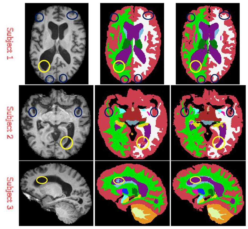
3 examples of AD Brain MRI and output labels (Each row is from one subject. 1st column is T1 MRI; 2nd column is WMV result; 3rd column is proposed result).

4. CONCLUSIONS

We have shown a principled approach to compute a non-stationary relaxation factor for the adaptive statistical atlas. This allows it to simultaneously segment 34 structures throughout the brain, including the subcortical structures. We have demonstrated the approach on healthy brains, achieving state of the art accuracy in a fraction of the time (100x speedup) as prior methods based on multi-atlas registrations. We have also tailored the approach for diseased brains, which is problematic even for multi-atlas based methods. By using our hybrid WMV-EASA method, we find obvious visible improvements throughout diseased brains for multiple structures including WM, ventricles and the cortex. Future work entails incorporating other models (e.g. sparse model [7]) to improve accuracy and utilizing derived values (e.g. volume-try) from our segmentations to predict disease stage and help guide treatment.