Measuring global spatial autocorrelation with data reliability information

Abstract

Assessing spatial autocorrelation (SA) of statistical estimates such as means is a common practice in spatial analysis and statistics. Popular spatial autocorrelation statistics implicitly assume that the reliability of the estimates is irrelevant. Users of these SA statistics also ignore the reliability of the estimates. Using empirical and simulated data, we demonstrate that current SA statistics tend to overestimate SA when errors of the estimates are not considered. We argue that when assessing SA of estimates with error, it is essentially comparing distributions in terms of their means and standard errors. Using the concept of the Bhattacharyya coefficient, we proposed the Spatial Bhattacharyya coefficient (SBC) and suggested that it should be used to evaluate the SA of estimates together with their errors. A permutation test is proposed to evaluate its significance. We concluded that the SBC more accurately and robustly reflects the magnitude of SA than traditional SA measures by incorporating errors of estimates in the evaluation.

An important theme in spatial analysis and statistics is to determine whether or not values across units within a study region are strongly correlated because the significant presence of spatial autocorrelation (SA) in the data violates the basic assumption of independence in classical statistics. In practice, Moran’s I (MC) and the Geary Ratio (GR) are regarded as standard measures to reflect the magnitude of SA of a study region (Cliff and Ord 1981). To evaluate the magnitude of SA, statistical estimates (“estimates” thereafter) derived from samples within neighborhoods are compared. When these statistics are applied, users often implicitly assume that estimates are accurate without error, while in reality all sample estimates have standard errors reflecting their degrees of uncertainty. In addition, when testing the significance of SA statistics, the difference between the observed and expected measures are standardized by the variances of the respective statistics. The analytical derivations of these variances implicitly assume that the estimates have unit variances or uniform variance across units (Cliff and Ord 1973, p.34).

It is the norm rather than the exception that the standard errors of estimates are not spatially uniform or random (e.g., Spielman and Folch 2015) but are not always provided with the data. However, standard errors should be included in the data because they reflect the reliability of the estimates. Increasing number of datasets gathered by government agencies (e.g., the American Community Survey (ACS) data disseminated by the U.S. Census Bureau) and private organizations (e.g., the State of Obesity datasets disseminated by the Trust of America’s Health & R. W. Johnson Foundation) include standard errors of the estimates. Thus, using existing measures to evaluate the level of SA of these spatial datasets fails to utilize the actual reliability information provided by the data, and the results from these existing measures are likely biased.

The objective of this study is to explore and demonstrate that when using existing measures to assess the SA of statistical estimates, results are insensitive to the error levels of the estimates as reflected by their standard errors. The insensitivity of results may also imply that the SA indicated by these measures is biased. Using simulated and empirical data, the relationship is explored between the magnitude of estimate error and the direction and magnitude of bias. Existing measures are not sufficient to reflect the SA of statistical estimates with uncertainty information. Therefore, a new measure is proposed to evaluate the SA of statistical estimates by considering the standard error associated with each estimate. This measure is based on the Bhattacharyya coefficient (BC), which measures the overlap between two distributions. It is demonstrated that the spatial Bhattacharyya coefficient (SBC) is a more statistically sufficient measure than existing SA measures because it considers the errors of statistical estimates in evaluating SA.

Uncertainty and SA measurement

Positional and attribute uncertainties, the two main sources among various types of uncertainty in spatial data (ANSI 1998), can influence SA measures because SA compares attributes over space. The impacts of positional uncertainty on SA have been explored in several empirical studies. Burra et al. (2002) examine the positional uncertainty of geocoded points and its impact on the results of global and local SA measures (i.e., MC, local Moran, G_i and G_i*). They report that even a low level of positional inaccuracy affects local SA measures, but that global measures are robust. Spatial weights matrix captures the spatial relationship among locations for the calculation of SA measures. When created from geocoded points with positional errors (Jacquez and Rommel 2009), errors originated from positional inaccuracy may propagate to SA measures. More recently, Griffith, Chun, and Lee (2016) investigated the impacts of positional uncertainty on local SA measures, including local Moran and G_i*, using heavy metal soil sample points. They found considerable changes of SA levels caused by positional uncertainty; specifically, changes in local Moran values were larger than in G_i*. Unlike positional uncertainty, the impact of attribute uncertainty on SA measures has not been extensively investigated, although its effects on the result of general spatial analysis are widely recognized (e.g., Haining and Arbia 1993; Griffith et al. 2007; Lee, Chun, and Griffith 2018).

Among various approaches to address attribute uncertainty in spatial analysis and statistics (Longley et al. 2011), a popular approach is to use a probability distribution function to represent attribute error as a form of an uncertain object (Heuvelink, Brown, and van Loon 2007). For example, Heuvelink (1998) developed various types of probability models for attribute error to reflect different measurement scales and space-time variability of an attribute, and implemented these models in geographic information science (GIS). In data mining, this uncertain object approach is widely used for cluster analysis, such as in the implementations of UK-means (Chau et al. 2006) and Fuzzy DBSCAN (Kriegel and Pfeifle 2005) methods. Specifically, these cluster analysis methods use a probability density function to calculate distance between each pair of uncertain objects instead of a general Euclidean distance (Kriegel and Pfeifle 2005). The research reported here also adopts the concept of uncertain objects, but in the attribute space (based on a probability density function) and develops an alternative SA measure by comparing probability density functions rather than only estimates.

Limitations of traditional SA measures for estimates with empirical error information

In the formulation of SA statistics, the differences between estimates are expressed as deviations from the mean (i.e., MC) and as actual differences (i.e., GR). Similarity between estimates is evaluated with the implicit assumption that estimates are relatively accurate. The standard errors of these estimates are not considered when the estimates are compared. Figure 1 illustrates the amount of overlapping probability density functions between two neighboring spatial units. Estimates in Figures 1A and1B are relatively similar as compared to those in Figures 1C and1D. If estimates have relatively small errors (narrower distributions in Figures 1B and1D) or if their errors are ignored, the similarity of these estimates, SA, is higher than those estimates with larger errors (wider distributions in Figures 1A and1C). Thus, the SA statistics of estimates are inflated when errors of estimates are not considered. By extension, estimates with larger errors are less positively autocorrelated than the same set of estimates with smaller errors. Conversely, when estimates with moderately strong negative SA (i.e., very different estimates), they should become more statistically similar if they have relatively larger errors (i.e., more positive or less negative autocorrelation) than as if they have smaller or no error.

Figure 1.

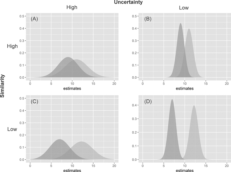
Illustrations of overlapping probability density functions between two neighboring spatial units with different levels of similarity and uncertainty in estimates.

In general, estimates with larger errors vary over larger ranges or more dissimilar, or the autocorrelation levels are diluted regardless if they are positively or negatively autocorrelated. In other words, if the errors of estimates are ignored in evaluating SA, it is similar to treating the estimates as highly accurate or without error, and the results tend to be more extreme. Statistical estimates with positive SA yield SA statistics more positive than they should while estimates with negative SA result in more negative SA statistics.

The second issue with using MC and GR is that in testing the significance of these statistics, the variances are assumed to be unity or constant. With no empirical information about the reliability of estimates, adopting these assumptions (i.e., uniform variance with unity) is reasonable. However, the analytical variances which adopt these assumptions likely create bias in testing the significance of the statistics. For example, the significance of MC can be biased due to the uncertainty of rates associated with the varying sizes of population at risk, and modified MC calculations for rates were proposed to address this uncertainty (Oden 1995; Waldhör 1996; Assunção and Reis 1999). It has been demonstrated that the uncertainty introduced by varying sample sizes is controllable using funnel plots (Dover and Schopflocher 2011). These treatments on the impacts of uncertainty on SA measures rely on known sample sizes, which may not be available. The research reported here examines the impacts of uncertainty on traditional SA measures using empirical (e.g., ACS data) and simulated data with varying degrees of reliability as reflected by the standard error values or related measures.

Biases of traditional SA measures when error information of estimates is ignored

Using the American Community Survey (ACS) data

The ACS data are used in this demonstration because each ACS’ estimate has a margin of error (MOE) indicating the reliability of estimate. The specific ACS datasets are the 5-year (2009–2014) estimates of median household income (MedInc) of counties in Texas, and estimates of median income of Hispanics households (HispInc) of census tracts from Dallas County, Texas (Figure 2). Table 1 shows the summary statistics of the two variables. The expected value of MC is $-1/\left(n-1\right)$ , where n is the number of spatial units. The range of MC is approximately between −1 and 1. An MC value greater than the expected value indicates a positive SA, and a value smaller than the expected value indicates a negative SA. The expected value of GR = 1, and the range of GR is between 0 and 2, with a value less than 1 indicating a positive SA and a value greater than 1 indicating a negative SA. While MC and GR offer consistent results (Table 1), both variables have a significant positive SA. However, MedInc of Texas counties has a stronger positive SA than HispInc in Dallas. The reliability of ACS estimates is closely related to the number of completed questionnaires, a combination of population size and response rate (U.S. Census Bureau 2009). Because the number of completed surveys is larger for larger spatial units, ACS estimates are more reliable for larger (e.g., counties) than for smaller units (e.g., census tracts) (Spielman and Folch 2015). Thus, it is not surprising that the average coefficient of variation (CV) of the county variable (0.0605) is much smaller than the average CV of the tract variable (0.2960).

Figure 2.

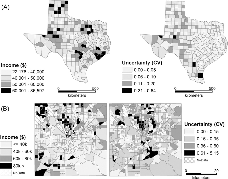
Sample ACS datasets: (A) median household income and CV values of Texas counties; (B) median income of Hispanic households and CV values in Dallas County, Texas.

Table 1.

Summary statistics of the two ACS variables for Texas counties (median household income, MedInc) and tracts in Dallas County, Texas (median income of Hispanic households, HispInc).

Dataset	# of areal units	Average estimates	SA measures		Average CV1	Min CV	Max CV	STD3 CV
			MC	GR
MedInc	254	46,353	0.4130 (<0.001)	0.5853 (<0.001)	0.0605	0.0039	0.6414	0.0577
HispInc	5162	49,355	0.2797 (<0.001)	0.6898 (<0.001)	0.2960	0.0023	5.1461	0.4207

¹CV- coefficient of variation

²Exclude tracts with missing data

³STD - standard deviation

The SA statistics (Table 1) are the levels of SA without considering error in the ACS estimates. If errors of estimates are considered, the true values of observations should vary according to their error levels. To demonstrate how the estimates may vary by incorporating the error information, the original estimate of each observation is replaced by a new estimate generated from a normal distribution with the mean and standard deviation corresponding to the original estimate and standard error of the observation, respectively. This normality assumption is reasonable given that that ACS estimates follows a normal distribution (U.S. Census Bureau 2009). This process to introduce error into an estimate is performed for each ACS estimate 1,000 times to create 1,000 sets of new estimates with empirical errors. For each set of estimates, we computed the MC and GR. The histograms in Figure 3 show the distributions of the two SA statistics with 1,000 sets of new estimates.

Figure 3.

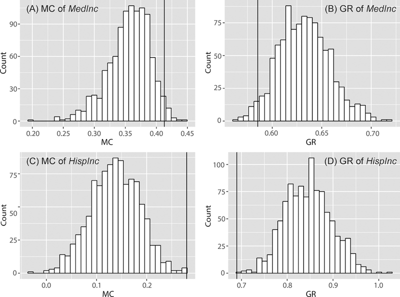
The distributions of MC [(A) and (C)] and GR [(B) and (D)] of the 1,000 sets of new estimates of the two variables generated by incorporating errors into the estimates. The MC and GR values without error information are shown by the vertical lines.

With the empirical errors introduced, most values of the two SA statistics for the Texas county data are more strongly positive than the tract data for Dallas County, consistent with the results using estimates without errors. However, by introducing errors to the estimates, the means of MC and GR are 0.3560 and 0.6322 for Texas counties (versus 0.4130 and 0.5853 for MC and GR of the original estimates, respectively) and 0.1364 and 0.8458 for the tracts (versus 0.2797 and 0.6898 for MC and GR of the original estimates, respectively) in Dallas County. The SA statistics for the estimates without considering error are biased upward (i.e., more positively autocorrelated) when compared to estimates with errors (Figure 2). In other words, if errors are ignored in estimates, the evaluation of SA is likely inflated.

Synthetic data

The above demonstrates that ignoring errors in estimates likely inflate SA values, resulting in stronger positive SA statistics than considering the errors in the statistical estimates. However, empirical data have mild to moderate levels of positive SA (Table 1). Although one expects that ignoring errors in the estimates likely results in less negatively autocorrelation if the estimates have negative SA, empirical data with true negative SA are rare (Griffith 2000). Therefore, this study simulates data with a negative SA to test our conceptual arguments. In addition, this simulation illustrates the impact of error on SA statistics with various SA and error levels. Simulation experiments are commonly used to test the properties of SA statistics (e.g., using different forms of spatial weights and sample sizes (Anselin and Florax 1995), and varying densities of weight matrices (Mizruchi and Neuman 2008; Smith 2009)).

The simulated data are generated based on two different processes, one for estimates and the other for associated variances. Spatially autocorrelated estimates are generated using a spatial autoregressive (SAR) process (Chun et al. 2016) as follows:

$$Y=1{\beta }_o+{\left(I-\rho W\right)}^{-1}\mathrm{\epsilon }$$

where $W$ is a row-standardized spatial weights matrix, $\epsilon$ is a vector of iid normal random errors, $\rho$ is a SA parameter and ${\beta }_o$ is set to one. Nine different $\rho$ values are used (−0.8, −0.6, −0.4, −0.2, 0, 0.2, 0.4, 0.6, 0.8), corresponding to the autocorrelation levels of the simulated estimates. Simulated values of each autocorrelation level are generated and distributed over three different sizes of regular hexagonal tessellations: 10-by-10, 30-by-30 and 50-by-50 (i.e., 100, 900, 2,500 observations, in series).

Subsequently, the nine sets of spatially autocorrelated values for each tessellation are paired with different levels of error. As CV indicates the relative amount of error associated with the estimates (i.e. $\text{CV}=standarderror/estimate$ ,) (Sun and Wong 2010; Spielman and Folch 2015), CV values are randomly generated from a truncated normal distribution with a lower truncation point equal to 0, and an upper truncation point equal to 2. The criteria for an appropriate CV level have not been formally investigated except in a small number of studies. The National Research Council suggests that a CV of 10–12% or less has a reasonable reliability (Citro & Kalton, 2007). ESRI (2014) states that a CV less than 12% indicates high reliability, 12–40% indicates moderate reliability, and over 40% indicates low reliability. Thus, the simulations employed six CV levels from 10% to 60% with an increment of 10%. The CV values are obtained from six different truncated normal distributions, whose means are 0.1, 0.2, 0.3, 0.4, 0.5 and 0.6. These means are primarily related to the above CV levels. The same standard deviations (0.1) are used for each distribution to minimize the impact of CV variability when the focus is on the impact of different CV (error) levels. As a result, a total of 162 sets of samples are generated with nine SA levels, six CV levels and three tessellation sizes. Note that the appropriateness of CV level depends on context or application.

Using the same process to incorporate errors to the estimates in the above ACS data, the original estimates of the 54 sets of samples (nine SA and six CV levels) of each tessellation are replaced with newly generated estimates (i.e., randomly drawn values). Each new estimate is drawn from a normal distribution, with the mean and standard deviation set to the original estimate and the standard error derived from its original CV values. This process is repeated 1,000 times for each estimate.

The variances of both MC and GR values decrease with increasing sample size from 100 (Figure 4A and B) to 2,500 (Figure 4E and F). However, when the SA are positive (ρ > 0), the original SA statistics are concentrated on the positive ends of the SA distributions (i.e., larger MC and smaller GR values). When the SA levels are negative (ρ < 0), the original SA statistics are on the negative ends of the SA distributions (i.e., smaller MC vales and larger GR values). In other words, when computing MC and GR without considering errors for estimates with positive SA, the computed statistics are more positively autocorrelated than they should be. Conversely, if the estimates are negatively spatially autocorrelated and errors are ignored, the computed SA statistics are more negatively autocorrelated than they should be. These results confirm the argument that ignoring errors in evaluating SA results in a statistical liability.

Figure 4.

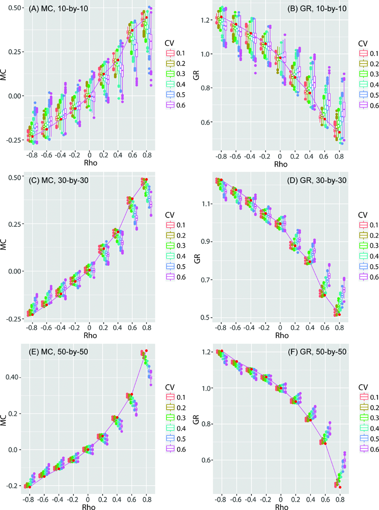
The distributions of MC and GR for the 1,000 sets of the random samples generated by incorporating errors into the estimates. The (red) points connected by line segments represent the SA statistics of the original simulated estimates (54 of them). The boxplots show the distributions of the SA statistics of estimates generated with errors.

The interplay of the error level of the SA estimate with sample size also affects the probability of detecting a significant SA. To address this interplay, the percentages of significant SA statistics with a p-value less than 0.01 based on a two-tail test in the previous simulation experiment are illustrated in Figure 5. In this graph 100% means all SA statistics from the simulation test are significant while 0% means all simulated SA statistics are not significant. With a larger sample size (i.e., 50-by-50 tessellation), SA is significant with a low value of ρ, and the significance is not influenced by the error levels. However, with smaller sample sizes (i.e., 10-by-10, 30-by-30 tessellations) the probability of detecting a significant SA decreases when the error level is high (e.g., CV = 0.6). This impact of error level is stronger for negative SA. Therefore, error in estimates have a strong influence on the detection of SA and cannot be ignored in assessing SA, especially when working with small sample sizes (e.g., less than 100 observations) and data with negative SA.

Figure 5.

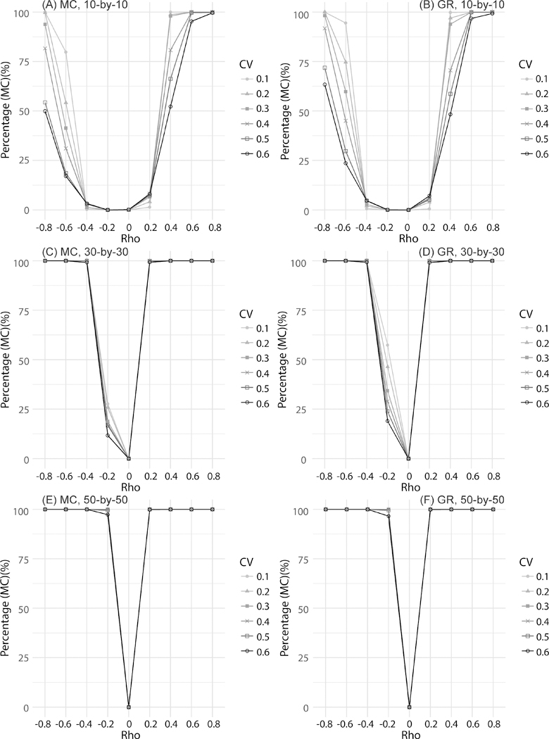
The percentages of significant SA values of the simulation dataset (p-value < 0.01)

In sum, if errors in estimates are ignored in evaluating SA using traditional measures, the results are likely biased toward the extremes (i.e., more positive autocorrelation for positive SA estimates, and more negative autocorrelation for negative SA estimates), based on the results of our analyses with the empirical (i.e., ACS data) and synthetic data. Also, the likelihood of having a significant SA statistic is inversely related to the magnitudes of errors of the estimates. To obtain a more accurate assessment of SA for estimates with error information using traditional measures such as MC and GR, the process of incorporating errors into the estimates with randomization is needed. However, the process of introducing variability to the estimates with empirical errors is time and computationally intensive, and an alternative approach is to derive an SA measure accounting for the errors of estimates.

Measuring spatial autocorrelation by accounting for error information

An alternative SA Measure

A major limitation of traditional SA measures is that when those SA measures compare estimates, do not consider the errors of the estimates when comparing the estimates. A more accurate comparison should include the error information, and a candidate to measure the difference between estimates and the errors of estimates is the Bhattacharyya coefficient (BC) or Bhattacharyya distance (BD). The BC or BD quantifies the dis/similarity between two discrete or continuous probability distributions (Bhalerao and Rajpoot 2003) and is widely used for image processing and pattern recognition (e.g., Kailath 1967; Schmidt and Skidmore 2003; Mas et al. 2004; Patra et al. 2015). Recently, the BD was used to derive class breaks in map classification while considering attribute error (Koo, Chun, and Griffith 2017; Wei, Tong, and Phillips 2017). Specifically, BC measures the similarity between the overlap between two distributions. Assuming $i\left(x\right)$ and $j\left(x\right)$ are two continuous distributions, according to Kailath (1967), BC is defined as follows:

$$\text{BC}\left(i,j\right)=\int \sqrt{i\left(x\right)j\left(x\right)}dx$$ (1)

The BD between two normal distributions is derived from this formulation (Coleman and Andrews 1979) as follows:

$$\text{BD}\left(i,j\right)=\frac{1}{4}\ln \left(\frac{1}{4}\left(\frac{{\sigma }_i^2}{{\sigma }_j^2}+\frac{{\sigma }_j^2}{{\sigma }_i^2}+2\right)\right)+\frac{1}{4}\left(\frac{{\left({\mu }_i-{\mu }_j\right)}^2}{{\sigma }_i^2+{\sigma }_j^2}\right)$$ (2)

where ${\mu }_i$ and ${\mu }_j$ are the sample estimates at locations $i$ and $j$ , respectively, ${\sigma }_i$ and ${\sigma }_j$ are the standard errors of the estimates at the corresponding locations and $ln$ denotes the natural logarithm. The BC has a negative exponential relationship to BD (Kailath 1967) as follows:

$$\text{BC}\left(i,j\right)=-\text{exp}\left(\text{BD}\left(i,j\right)\right)=\sqrt{\frac{2{\sigma }_i{\sigma }_j}{{\sigma }_i^2+{\sigma }_j^2}}{e}^{\frac{1}{4}\frac{{\left({\mu }_i-{\mu }_j\right)}^2}{{\sigma }_i^2+{\sigma }_j^2}}.$$ (3)

The value of BC, which indicates the amount of overlap between two sample distributions, ranges from 0 to 1 where. 0 indicates no overlap and 1 indicates a perfect overlap. Thus, BC is a comprehensive index to measure the difference between two distributions by considering both their means and deviations.

Using BC, a global SA measure (Spatial Bhattacharyya coefficient (SBC)) is formulated as follows:

$$\text{SBC}=\frac{{\sum }_{i=1}^n{{\displaystyle \sum }}_{j=1}^n{w}_{ij}\text{BC}\left(i,j\right)}{{{\displaystyle \sum }}_{i=1}^n{{\displaystyle \sum }}_{j=1}^n{w}_{ij}}=\frac{n}{{{\displaystyle \sum }}_{i=1}^n{{\displaystyle \sum }}_{j=1}^n{w}_{ij}}·\frac{{{\displaystyle \sum }}_{i=1}^n{{\displaystyle \sum }}_{j=1}^n{w}_{ij}\text{BC}\left(i,j\right)}{{{\displaystyle \sum }}_{i=1}^n\text{BC}\left(i,i\right)},$$ (4)

where $w_{ij}$ is an element of a spatial weights matrix that has a binary weight (i.e., 0 and 1), n is the total number of observations, and ${\displaystyle {\sum }_{i=1}^n\text{BC}\left(i,i\right)=n}$ . The expression on the right hand side of Equation 4 shows a conceptual similarity to the general SA statistics, specifically to MC. The SBC ranges from 0 to1, with a higher SBC indicating a high degree of similarity between the neighboring distributions. That is, SBC values are affected by both error and SA levels. A higher error level would yield a higher SBC value, and in contrast, a lower error level would lead to a lower SBC value. In addition, positive SA of estimates would lead to a high SBC value, while negative SA of estimates would lead to a low SBC value, keeping the error level constant. The significance of SBC is conducted through a permutation test. The SBC formulation is similar to MC and GR conceptually in that all numerators capture the differences between neighboring observations. However, the numerators of MC and GR consider only the estimates, while SBC considers both the estimates and errors. Thus, comparing the values of MC and GR with SBC needs to acknowledge the conceptual difference between the two types of SA measures.

Using SBC to evaluate SA of estimates with error information

The property of SBC is explored with simulated data consisting of spatial autocorrelated estimates and error statistics. Data generation is similar to the process described in Section 4.2 as the spatially autocorrelated estimates are generated through an SAR process with nine different autocorrelation levels ( $\rho$ = −0.8, −0.6, −0.4, −0.2, 0.0, 0.2, 0.4, 0.6 and 0.8). Standard errors are derived from CV values drawn from a truncated normal distribution with different means (0.1, 0.2, 0.3, 0.4, 0.5 and 0.6) and a fixed standard deviation (0.1). The 1,000 sets of spatially autocorrelated estimates and associated standard errors are generated for each pair of $\rho$ and CV values, with a total of 54,000 simulation datasets generated for three different sample sizes: 10-by-10, 30-by-30 and 50-by-50 regular hexagonal tessellations. The MC and GR values for the simulation datasets show that as $\rho$ increases the SA level of the estimates increases (Figure 6). The increase tends to be less for negative and low SA but more for positive and high SA. However, CV levels do not affect the MC values because MC does not consider errors of estimates.

Figure 6.

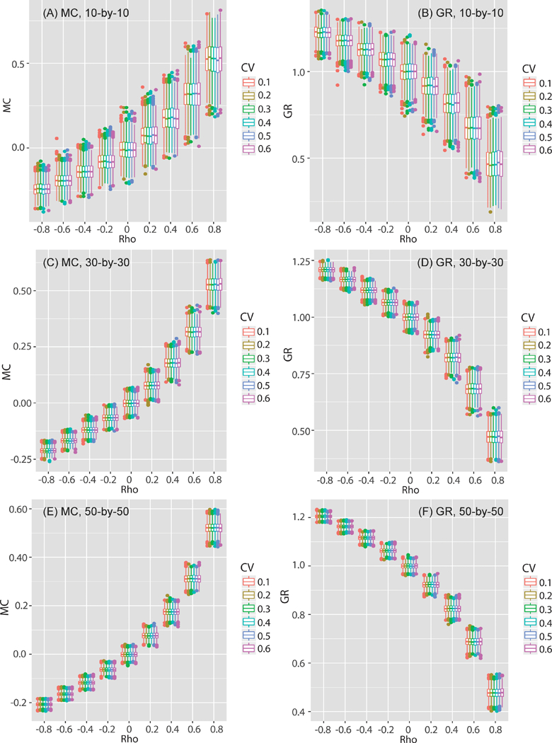
The box-whisker plots of estimated MC and GR values of the simulation datasets with different levels of spatial autocorrelatoin (ρ).

Figure 7 shows the distributions of SBC with different SA ( $\rho$ ) and error (CV) levels. Three salient observations are offered by Figures 6 and 7. First, the SBC means become larger with increasing SA as reflected by the traditional measures of GR and MC (Figure 6). The increases are much larger for strong and positive SA than for negative or weak positive SA. Such a pattern is also similar for the GR and MC results (Figure 6). Second, the SBC means are markedly affected by the error level (i.e., CV) given any SA level (i.e., ρ). Smaller CV levels generally lead to lower SBC values, and larger CV values lead to larger SBC values. Also, the range of SBC values is affected by the SA level. For instance, with a strongly negative SA (i.e., ρ = –0.8), the mean SBC ranges from 0.07 to 0.40. When SA is strongly positive at ρ = 0.8, the mean SBC ranges from 0.15 to 0.56. Third, the variability of SBC is associated with both ρ and CV. A larger ρ value tends to produce larger variation in SBC than a smaller ρ. With both large ρ and CV values, the SBC have the largest variability. Also, the variability of SBC shows a strong association to sample size, a characteristic generally shared among SA statistics (Figure 6). Specifically, SBC shows a smaller variance with a larger sample size (i.e., 50-by-50 tessellation) than that with a smaller sample size (i.e., 10-by-10 tessellation).

Figure 7.

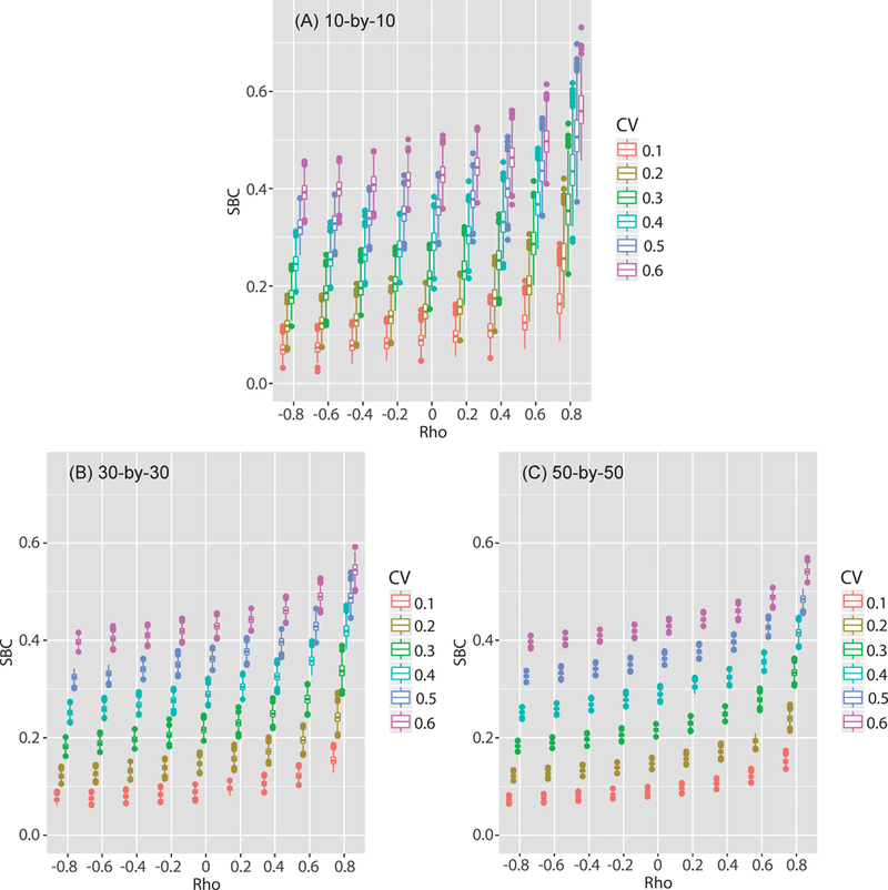
The box-whisker plots of estimated SBC of the simulation datasets with different levels of spatial autocorrelation (ρ).

These results are consistent with the proposal that SBC is a sufficient measure of SA. When estimates have strong negative SA (i.e., negative ρ) and are relatively reliable (i.e., low CV values), these estimates should be statistically different and their corresponding distributions should have low SA values (SBC). If these negatively autocorrelated estimates are relatively unreliable (i.e., large CV values), they are more similar to each other (i.e., larger overlaps in their distributions) or are more spatially autocorrelated than those distributions with more reliable estimates (i.e., smaller overlaps). It follows that these negatively autocorrelated estimates may not be statistically different. Thus large CV values or having more unreliable estimates make the distributions more similar and, therefore, produce larger SBC values. A larger ρ value for the estimates raises the similarity between neighboring estimates, but the errors of the estimates (i.e., uncertainty) are critical in determining SBC values.

A permutation test examines the statistical power of SBC in detecting significant SA among neighboring estimates with their errors. For each simulation dataset (54,000 datasets), the permutation shuffles the estimates and standard errors separately 1,000 times. The mean probabilities of SBC values from the permutation test (10-by-10 tessellation in Figure 8A) show that when estimates have a negative SA (i.e., negative ρ) and are relatively reliable (i.e., low CV), their corresponding SBC values are likely to be significant with p > 0.975. However, it is difficult to statistically differentiate unreliable estimates from one other (e.g., CV = 0.6) even with strong negative SA (ρ = −0.8). When ρ is positive (i.e., positive SA) and the CV is relatively large (i.e., unreliable estimates), the SBC tends to be significant, indicating a similarity among neighboring distributions (i.e., comparing estimates together with their errors). Similar to other SA statistics, the level of significance in SBC is greater when sample size is large (Lin, Lucas, and Shmueli 2013). For the 50-by-50 tessellation (Figure 8C), SBCs are significant even with a large CV (i.e., CV = 0.6), although the estimates do not show spatial autocorrelation (i.e., ρ = 0.0). This suggests that the estimate errors have an overwhelming influence on determining the presence of positive SA among distributions.

Figure 8.

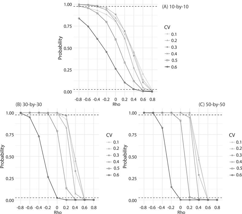
The mean probabilities of SBC of the simulation datasets from the permutation test (the dotted lines are 95% confidence intervals for a two-tail test.)

Application to the ACS data

The SBCs are computed for the two ACS datasets in Section 4 (MedInc at the county level and HispInc at the census tract level) and the MC, GR and CV of the two variables are included for comparison purpose (Table 2). MC and GR consistently show that MedInc has stronger positive SA than HispInc. However, SBC values indicate that HispInc are more similar than MedInc as the SBC for MedInc is 0.405 and that for HispInc is 0.618. In general, a coarser areal tessellation tends to have a higher SA as data are relatively smoother than that found in a finer areal tessellation where data have more local variation. Although MC and GR conform to this general expectation, these statistics do not consider the errors of the estimates. The mean CV of MedInc is small (0.0605), while that of HispInc is relatively large (0.2960) (Table 2). Given that the tract-level estimates have high levels of error, estimates can be statistically similar when errors are taken into consideration. Thus, the SBC for HispInc is relatively large when compared to the SBC for MedInc, in which the values are more likely to be statistically different with small error levels. The permutation tests also indicate that the two SBC values are statistically significant (Figure 9 and Table 2).

Table 2.

SBC values and their probabilities for two ACS variables, MedInc and HispInc.

Dataset	SA	Mean CV	SBC	p-value
MedInc	MC: 0.4130 (<0.001) GR: 0.5853 (<0.001)	0.0605	0.4046	0.001
HispInc	MC: 0.2797 (<0.001) GR: 0.6898 (<0.001)	0.2960	0.6184	0.001

Figure 9.

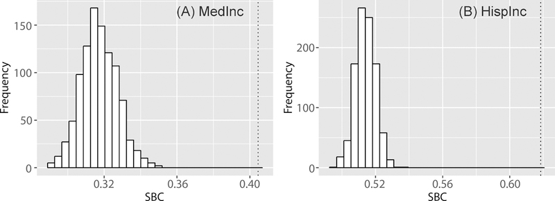
The distributions of SBCs from the permutation tests for the two ACS variables, MedInc and HispInc. The two dotted vertical lines represent the SBC values for corresponding variables.

Conclusion

When using popular statistics to evaluate the SA of estimates, which are often the means of statistical distributions, and the norm is that the reliability levels of the estimates (represented by the corresponding standard error or CV levels) are ignored. Comparison of these estimates, therefore, assumes that the estimate errors are uniform. Their errors and variability are not considered, and as a result the SA assessment is biased upward. If the estimate errors are considered in assessing SA level, the process is conceptually the same as comparing distributions with respect to the means and standard errors.

The applicability of BC to comparing distributions is recognized, and subsequently the SBC is proposed as a measure of SA. Using simulated and ACS data, the utility of SBC in evaluating the SA of distributions is demonstrated. In general, SBC captures a high SA when the distributions (or estimates) have large errors. When errors are relatively small, the SA of distributions depends more on the similarity of estimates (i.e., means) than the errors. The significance test of SBC is conducted with the permutation test. When an SA assessment is needed for data with relatively large errors (e.g., mean CV over 40%) or errors with considerable variability, it is proposed that SBC¹ be used to capture error information. Taking a slightly more conservative position, even if estimates have relatively low error but are relatively non-uniform, SA assessment should employ SBC in concert with traditional SA measures. Moreover, SBC furnishes an additional SA measure highlighting the influence of errors on existing SA statistics (i.e., MC and GR).

The proposed measure furnishes a new approach to measuring SA. Instead of comparing estimates (i.e., means) as in conventional SA statistics (e.g., MC, GR, G-statistic, Local spatial heteroscedasticity measure (LOSH, Ord and Getis 2012)), the proposed approach highlights the importance of considering the distributions underneath the estimates. As the new approach requires one to consider the error of estimate as an additional component in SA evaluation, the proposed SA statistic-SBC-is not compatible with the more conventional approaches to assess SA, particularly in determining the direction of autocorrelation. The traditional dichotomous concept of positive-negative SA is no longer applicable in comparing distributions, although the concept is still relevant in describing estimates.

Future studies should pursue along several directions. First, the significance test for SBC is conducted based on a permutation test. However, permutation might be limited when the distribution of a variable is affected by other factors, such as the underlying population at risk (Waller and Gotway 2004). Thus, a conditional test has merit to reflect the underlying distribution of a variable. Second, the impact of error on the SBC warrants further investigation with a weighting scheme between the error level and the similarity of estimates. The SBC appears to be more affected by the error level than the similarity of estimates. If the SBC approach allows analysts to interactively adjust the relative weights for error and the similarity of estimates, then the influence of errors and the similarity of estimates on SA can be evaluated separately. However, in the current formulation of SBC, standard errors and estimates cannot be linearly disentangled (i.e., weights for errors and estimate similarity cannot be controlled independently). Future studies are warranted to derive a more flexible scheme to control the influences of these two components in assessing the SA of distributions. The study provides evidence that when estimate error is available, SBC should be employed to assess SA. Thus, a future research is to derive more specific quantitative guidelines to determine the circumstances when SBC and traditional SA measures yield significantly different results.

Biography

HYEONGMO KOO was a PhD student at the University of Texas at Dallas 75080 and is currently a Postdoctoral Research Associate in the Key Laboratory of Virtual Geographic Environment at Nanjing Normal University, Nanjing, Jiangsu Province, China 210046. hmo.koo@gmail.com. His research interests include in geovisualization, spatial data uncertainty, and GIS focusing on urban and economic issues.

DAVID W. S. WONG is a Professor in the Department of Geography and Geoinformation Science at George Mason University, Fairfax, VA 22030. dwong2@gmu.edu. His research interests include measuring spatial segregation, scale issues in spatial analysis, environmental health and assessment with GIS, attribute uncertainty in spatial data, and scientific visualization.

YONGWAN CHUN is an Associate Professor of Geospatial Information Sciences at the University of Texas at Dallas, Richardson, TX 75080. ywchun@utdallas.edu. His research interests lie in spatial statistics and GIS focusing on urban issues including population movement, environment, public health, and crime.

References

- Anselin L, and Florax RJGM. 1995. Small sample properties of tests for spatial dependence in regression models: some further results In New Directions in Spatial Econometrics. Advances in Spatial Science, eds. Anselin L and Florax RJGM, 21–74. Springer, Berlin, Heidelberg. [Google Scholar]
- ANSI (American National Standards Institute). 1998. Spatial Data Transfer Standard (SDTS) - Part 1. Logical specifications. Washington, D.C.: ANSI NCITS 320–1998. [Google Scholar]
- Assunção RM, and Reis EA. 1999. A new proposal to adjust Moran’s I for population density. Statistics in Medicine 18:2147–2162. [DOI] [PubMed] [Google Scholar]
- Bhalerao AH, and Rajpoot NM. 2003. Discriminant feature selection for texture classification In Proceedings of the British Machine Vision Conference 2003. United Kingdom. [Google Scholar]
- Burra T, Jerrett M, Burnett RT, and Anderson M. 2002. Conceptual and practical issues in the detection of local disease clusters: A study of mortality in Hamilton, Ontario. The Canadian Geographer 46 (2):160–171. [Google Scholar]
- Chau M, Cheng R, Kao B, and Ng J. 2006. Uncertain data mining: an example in clustering location data In Advances in Knowledge Discovery and Data Mining, Lecture Notes in Computer Science, eds. Ng WK, Kitsuregawa M, Li J, and Chang K, 199–204. Heidelberg: Springer. [Google Scholar]
- Chun Y, Griffith DA, Lee M, and Sinha P. 2016. Eigenvector selection with stepwise regression techniques to construct eigenvector spatial filters. Journal of Geographical Systems 18 (1):67–85. [Google Scholar]
- Citro CF, and Kalton G. 2007. Using the American Community Survey: Benefits and challenges. National Academy Press. [Google Scholar]
- Cliff AD, and Ord JK. 1973. Spatial autocorrelation, monographs in spatial environmental systems analysis. London, UK: Pion Limited. [Google Scholar]
- Cliff AD, and Ord JK. 1981. Spatial processes: models & applications. London: Pion. [Google Scholar]
- Coleman GB, and Andrews HC. 1979. Image segmentation by clustering. Proceedings of IEEE 67 (5):773–788. [Google Scholar]
- Dover DC, and Schopflocher DP. 2011. Using funnel plots in public health surveillance. Population Health Metrics 9:1–11. [DOI] [PMC free article] [PubMed] [Google Scholar]
- Environmental Systems Research Institute (ESRI). 2014. The American community survey. An ESRI white paper. [Google Scholar]
- Griffith DA 2000. A linear regression solution to the spatial autocorrelation problem. Journal of Geographical Systems 2 (2):141–156 [Google Scholar]
- Griffith DA, Chun Y, and Lee M. 2016. Locational error impacts on local spatial autocorrelation indices: A Syracuse soil sample Pb-level data case study In Proceedings of Spatial Accuracy 2016, eds. Bailly J-S, Griffith DA, and Josselin D, 136–143. Avignon, FR: UMR 7300 ESPACE. [Google Scholar]
- Griffith DA, Millones M, Vincent M, Johnson DL, and Hunt A. 2007. Impacts of positional error on spatial regression analysis: A case study of address locations in Syracuse, New York. Transactions in GIS 11 (5):655–679. [Google Scholar]
- Haining R, and Arbia G. 1993. Error propagation through map operations. Technometrics 35 (3):293–305. [Google Scholar]
- Heuvelink GBM 1998. Error propagation in environmental modelling with GIS. London, UK: Taylor & Francis. [Google Scholar]
- Heuvelink GBM, Brown JD, and van Loon EE. 2007. A probabilistic framework for representing and simulating uncertain environmental variables. International Journal of Geographical Information Science 21 (5):497–513. [Google Scholar]
- Jacquez GM, and Rommel R. 2009. Local indicators of geocoding accuracy (LIGA): theory and application. International Journal of Health Geographics 8:60. [DOI] [PMC free article] [PubMed] [Google Scholar]
- Kailath T 1967. The Divergence and Bhattacharyya Distance Measures in Signal Selection. IEEE Transactions on Communication Technology 15 (1):52–60. [Google Scholar]
- Koo H, Chun Y, and Griffith DA. 2017. Optimal map classification incorporating uncertainty information. Annals of the American Association of Geographers 107 (3):575–590. [Google Scholar]
- Kriegel H, and Pfeifle M. 2005. Density-based clustering of uncertain Data. In The 11th ACM SIGKDD International Conference on Konwledge Discovery in Data Mining, 672–677. Chicago. [Google Scholar]
- Lee M, Chun Y, and Griffith DA. 2018. Error propagation in spatial modeling of public health data: a simulation approach using pediatric blood lead level data for Syracuse, New York Environmental Geochemistry and Health. Advance online publication; 10.1007/s10653-017-0014-7. [DOI] [PubMed] [Google Scholar]
- Lin M, Lucas HC, and Shmueli G. 2013. Too big to fail: large samples and the p-value problem. Information Systems Research 24 (4):906–917. [Google Scholar]
- Longley PA, Goodchild MF, Maguire DJ, and Rhind DW. 2011. Geographical Information Systems and Science Third Edition. Hoboken, NJ: John Wiley & Sons. [Google Scholar]
- Mas JF, Puig H, Palacio JL, and Sosa-López A. 2004. Modelling deforestation using GIS and artificial neural networks. Environmental Modelling and Software 19 (5):461–471. [Google Scholar]
- Mizruchi MS, and Neuman EJ. 2008. The effect of density on the level of bias in the network autocorrelation model. Social Networks 30 (3):190–200. [Google Scholar]
- Oden N 1995. Adjusting Moran’s I for population density. Statistics in Medicine 14:17–26. [DOI] [PubMed] [Google Scholar]
- Ord JK, and Getis A. 2012. Local spatial heteroscedasticity (LOSH). Annals of Regional Science 48 (2):529–539. [Google Scholar]
- Patra BK, Launonen R, Ollikainen V, and Nandi S. 2015. A new similarity measure using Bhattacharyya coefficient for collaborative filtering in sparse data. Knowledge-Based Systems 82:163–177. [Google Scholar]
- Schmidt KS, and Skidmore AK. 2003. Spectral discrimination of vegetation types in a coastal wetland. Remote Sensing of Environment 85 (1):92–108. [Google Scholar]
- Smith TE 2009. Estimation bias in spatial models with strongly connected weight matrices. Geographical Analysis 41 (3):307–332. [Google Scholar]
- Spielman SE, and Folch DC. 2015. Reducing uncertainty in the American Community Survey through data-driven regionalization. PLoS ONE 10 (2):1–21. [DOI] [PMC free article] [PubMed] [Google Scholar]
- Sun M, and Wong DWS. 2010. Incorporating data quality information in mapping American Community Survey data. Cartography and Geographic Information Science 37 (4):285–299. [DOI] [PMC free article] [PubMed] [Google Scholar]
- U.S. Census Bureau. 2009. A Compass for Understanding and Using American Community Survey Data: What Researchers Need to Know. Washington, DC: U.S. Goverment Printing Office. [Google Scholar]
- Waldhör T 1996. The Spatial autocorrelation coefficient Moran’s I under Heteroscedasticity. Statistics in Medicine 15:887–892. [DOI] [PubMed] [Google Scholar]
- Waller LA, and Gotway CA. 2004. Applied Spatial Statistics for Public Health Data. Hoboken, NJ: John Wiley & Sons. [Google Scholar]
- Wei R, Tong D, and Phillips JM. 2017. An integrated classification scheme for mapping estimates and errors of estimation from the American Community Survey. Computers, Environment and Urban Systems 63:95–103. [Google Scholar]