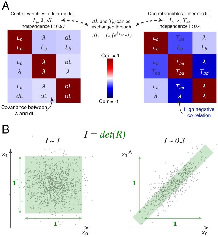
Figure 6. Decomposition method.

(A) The cell division cycle of a single cell can be described by different combinations of three variables which we refer to as decompositions. For example, the set $(L_b,dL,\lambda )$ corresponds to an adder decomposition, while $(L_b,T_{bd},\lambda )$ corresponds to a timer decomposition. For each possible decomposition, we can calculate the matrix $R$ of observed correlations $R_{ij}$ between each pair of variables in the decomposition from the data. Shown are the correlation matrices for the adder decomposition (left) and the timer decomposition (right), with positive correlations shown in red and negative correlations in blue. The independence $I$ of each decomposition is defined as the determined of the correlation matrix $I=\det (R)$ and is indicated on top of each matrix. While the independence for the adder decomposition is close to the possible maximum of 1, the independence of the timer correlation is much lower due to a strong negative correlation between growth rate $\lambda$ and the cell cycle duration $T_{bd}$. (B) Conceptual illustration of the independence measure $I$. For each decomposition, the data can be thought of as a scatter of points in the space of the decomposition’s variables, normalized such that the variance of points along each dimension is 1. In this conceptual example, we show two scatters of points for the two variables $x_0$ and $x_1$. The independence $I$ corresponds to the square of the volume covered by the scatter of points. On the left, there is virtually no correlation between the two variables, that is $R_{01}\approx 0$, such that the independence $I=\det (R)=1-R_{01}^2\approx 1$. In contrast, on the right there is a strong correlation, leading to a much lower independence $I\approx 0.3$. In this way, the independence measure quantifies to what extent the variables in the decomposition fluctuate independently, and this measure applies to scatters of any number of dimensions.

Figure 6—figure supplement 1. Correlation matrices for all decompositions of the division cycle.

In the main Figure 6, we showed the correlation matrices and independence measure for two possible decompositions of the division cycle. Here we show the correlation matrices for all eight possible decompositions, sorted by their independence $I$. Each matrix represents one decomposition, and each element of the matrix shows the correlation of the two variables indicated within it. The level and sign of correlation is given by the color bar.