

Abstract
In this paper, we aim to predict conversion and time-to-conversion of mild cognitive impairment (MCI) patients using multi-modal neuroimaging data and clinical data, via cross-sectional and longitudinal studies. However, such data are often heterogeneous, high-dimensional, noisy, and incomplete. We thus propose a framework that includes sparse feature selection, low-rank affinity pursuit denoising (LRAD), and low-rank matrix completion (LRMC) in this study. Specifically, we first use sparse linear regressions to remove unrelated features. Then, considering the heterogeneity of the MCI data, which can be assumed as a union of multiple subspaces, we propose to use a low rank subspace method (i.e., LRAD) to denoise the data. Finally, we employ LRMC algorithm with three data fitting terms and one inequality constraint for joint conversion and time-to-conversion predictions. Our framework aims to answer a very important but yet rarely explored question in AD study, i.e., when will the MCI convert to AD? This is different from survival analysis, which provides the probabilities of conversion at different time points that are mainly used for global analysis, while our time-to-conversion prediction is for each individual subject. Evaluations using the ADNI dataset indicate that our method outperforms conventional LRMC and other state-of-the-art methods. Our method achieves a maximal pMCI classification accuracy of 84% and time prediction correlation of 0.665.
Keywords: Matrix completion, Classification, Multi-task learning, Data imputation, Low-rank representation
1. Introduction
Alzheimer’s disease (AD) (Association et al., 2016, 2017) is the most prevalent dementia and is commonly associated with progressive memory loss and cognitive decline. It is incurable and requires attentive care, thus imposing significant socio-economic burden on many nations. It is thus vital to detect AD in its earliest stage before its onset for possible therapeutic treatment. The prodromal stage of AD, called mild cognitive impairment (MCI), is characterized by mild but measurable decline of memory and cognition. Studies show that some MCI patients will recover over time, but more than half will progress to dementia within five years (Gauthier et al., 2006). MCI patients that will progress to AD are retrospectively categorized as progressive MCI (pMCI) patients, whereas those who remain stable as MCI are categorized as stable MCI (sMCI). In this paper, we focus on differentiating pMCI from sMCI patients and predicting the time to the event of AD conversion.
Biomarkers based on different modalities, such as magnetic resonance imaging (MRI), positron emission topography (PET), and cerebrospinal fluid (CSF), have been widely studied for the prediction of AD progression (Zhang et al., 2012; Li et al., 2015; Weiner et al., 2013; Zhan et al., 2015; Li et al., 2014; Adeli-Mosabbeb et al., 2015; Huang et al., 2015; Zhu et al., 2015; 2016; Zhou et al., 2017; Zhu et al., 2017; Thung et al., 2016, 2017). The Alzheimer’s disease neuroimaging initiative (ADNI) collects these data longitudinally from subjects ranging from cognitively normal elderly subjects to AD patients in an effort to improve prediction of AD progression. However, these data are incomplete due to subject dropouts and unacquired modalities associated with factors such as study design and cost constraints. The easiest and most popular way to deal with missing data is by discarding incomplete samples (Zhang et al., 2012), which will however decrease sample size and statistical power. An alternative is to impute the missing data, via methods such as k-nearest neighbor (KNN), expectation maximization (EM), or low-rank matrix completion (LRMC) (Troyanskaya et al., 2001; Zhu et al., 2011; Candès and Recht, 2009; Sanroma et al., 2014). These imputation methods, however, do not perform well on data with blocks of missing values (Thung et al., 2014; Yuan et al., 2012; Yu et al., 2014), causing erroneous prediction outcomes.
To avoid the need for imputation, Yuan et al. (2012) proposed a method, called incomplete multiple source feature learning (iMSF), to first divide the data into disjoint subsets of complete data, and then jointly learn the classification or prediction models for these subsets. Through joint feature learning, iMSF enforces all subset classifiers to use a common set of features for each modality. However, this will cause samples with less number of modalities to have limited number of features when making prediction. In addition, using disjoint subsets of data will also cause small sample size issue for each prediction model (Xiang et al., 2014).
On the other hand, the method proposed by Goldberg et al. (2010) imputes the missing feature values and target values (e.g., diagnostic status and clinical scores) simultaneously using a low-rank assumption. All samples, including those with missing feature values, and their corresponding targets are concatenated into a matrix and the unknown values are then imputed via LRMC. This approach is able to make use of the incomplete samples more effectively. Thung et al. (2014) improved the efficiency and effectiveness of this method by performing feature and sample selection before matrix completion.
However, all these methods do not explicitly take into account the heterogeneous nature of the data. Recent studies (Markesbery, 2010; Nettiksimmons et al., 2013) show that there is significant biological heterogeneity among ADNI amnestic MCI patients. Some MCI subjects are biologically similar to normal aging subjects, while some have the characteristic AD’s pathologies, and some have other various late-life neurodegenerative pathologies (Nettiksimmons et al., 2013; Rahimi and Kovacs, 2014). Postmortem brain studies (Markesbery, 2010; Petersen et al., 2006; Jicha et al., 2006; Cairns et al., 2015) on deceased MCI and AD subjects also confirm that most of them developed a mixture of neurodegenerative diseases. The comorbidities (other than AD) include argyrophilic grain dementia, Lewy body dementia, Parkinson disease, hippocampal sclerosis, and frontotemporal dementia. These studies imply that not all MCI subjects are affected by the same AD pathologies.
In this study, we utilize longitudinal multi-modality data to capture the complexity and heterogeneity of AD pathology. The data are heterogeneous, prone to noise, and incomplete. To deal with these problems, we recently proposed an approach (Thung et al., 2015b) to cluster the data into subsets using low-rank representation (LRR) (Liu et al., 2013) and perform LRMC on the samples on each of these subsets separately, to improve the overall classification performance. This approach assumes that the data resides in a union of several low-dimensional subspaces, each spanned by a data subset, and tries to recover these subspaces through LRR. Each sample is assumed to reside in one of the subspaces. However, in reality, the samples can potentially reside across multiple subspaces (Markesbery, 2010). In addition, data clustering also reduces the number of samples associated with each subspace and hence may reduce the effectiveness of the prediction model. We have also demonstrated in (Thung et al., 2015b) that the prediction performance of the LRMC algorithm can also be improved by using a denoised version of the data, which can be obtained via LRR.
In this paper, we propose to use low-rank affinity pursuit denoising (LRAD) in combination with the sparse feature selection (FS) to improve the prediction power of LRMC for incomplete, noisy, and heterogeneous multi-modal data. More specifically, we use incomplete low-rank representation (ILRR) (Liu et al., 2013; Shi et al., 2014) for LRAD, where the samples are denoised by representing them using their neighboring points. In addition, we use lasso (Tibshirani, 1996; Liu et al., 2009a, 2009b; Liu and Ye, 2009) to select the most discriminative features for use in prediction. Lastly, we utilize LRMC to predict the output targets, which consist of diagnostic labels (i.e., pMCI/sMCI) and conversion times. We tested our framework using longitudinal and cross-sectional multimodality MRI data and confirm that the proposed method outperforms the conventional LRMC method and other state-of-the-art methods. It is also important to note that there are many hyper-parameters associated with LRMC. In this paper, we propose to use a Bayesian optimization framework to automatically select the best set of hyper-parameters. The contributions of this paper are threefold:
We propose a framework for pMCI diagnosis and conversion time prediction using longitudinal multi-modal data, which can be incomplete and noisy. In comparison, previous studies in the literature (Section 2.1) were often focusing on using either multi-modal or longitudinal data for pMCI diagnosis. Moreover, unlike our method which is applicable to incomplete datasets, most of the previous methods are only applicable to datasets without missing data. More importantly, time-to-conversion predictions in the literature are mostly used for global analysis based on statistical methods, while our study is one of the few non-statistical methods that addresses this issue at individual level. To the best of our knowledge, our study is the first to predict both the pMCI diagnosis and time-to-conversion jointly. To this end, we propose to employ sparse feature selection to remove outlier features, ILRR to denoise the data, and finally LRMC to predict the target outputs.
We propose a matrix completion algorithm that is able to predict the conversion time even when some of the data are missing and censored. The missing data issue is due to missing modalities at certain time points for some subjects. In addition, our sMCI data is censored, i.e., we are unsure whether the sMCI subject will progress to AD if we increase the monitoring period indefinitely. Conventional linear regression models are not applicable to censored data, while the conventional methods that work on these data (Section 2.2) only provide the “probability” of conversion. To this end, we design an LRMC algorithm with three data fitting terms, one for the input features, one for the diagnostic labels (binary targets), and one for the conversion time (continuous-valued targets), along with an additional inequality constraint. Our modified matrix completion algorithm enables us to predict the conversion time for the censored data (i.e., sMCI), by constraining their predicted values to be at least more than a specific value.
We employ a Bayesian optimization scheme to automatically select the optimal hyper-parameters for LRMC.
2. Related works
In this section, we briefly discuss the related previous research works.
2.1. MCI-to-AD conversion prediction
Many works (Wei et al., 2016; Stoub et al., 2004) use MRI data for MCI-to-AD conversion predictions. For example, Stoub et al. (2004) used MRI-derived entorhinal volume for prediction. Wei et al. (2016) used MRI and structural network features to predict MCI-to-AD conversion. They employed sparse linear regression with stability selection to select features and then used support vector machine (SVM) for classification. They used data at baseline, and 6, 12, and 18 months before diagnosis of probable AD for prediction. The best classification accuracy they obtained was 76% using the data 6 months prior to AD diagnosis. Misra et al. (2009) used longitudinal MRI data to extract brain temporal changes for detecting MCI-to-AD conversion. However, this study used follow-up data of very short period (i.e., up-to 15 months) with unbalanced data at each cohort (i.e., pMCI and sMCI).
Some works used multimodal data (e.g., MRI, PET, CSF, demographics, genetic data) for conversion prediction (Davatzikos et al., 2011; Cheng et al., 2015b, 2015a; Dukart et al., 2016; Moradi et al., 2015). Cheng et al. (2015b), for example, used MRI, PET, and CSF data in their studies. They employed transfer learning to borrow information from other related cohorts, i.e., AD and NC, to help select the features from MCI cohorts for MCI-to-AD conversion prediction, achieving 79% prediction accuracy. In another similar work, Cheng et al. (2015a) employed multimodal manifold-regularized transfer learning for feature selection, and achieved 80% accuracy in conversion prediction. Xu et al. (2016) used modality-weighted sparse representation-based classification method to combine data from MRI, fluorodeoxyglucose PET, and florbetapir PET, and achieved 82.5% prediction accuracy. They defined pMCI as MCI subjects that progressed to MCI within 36 months, and defined the remaining MCI subjects as sMCI. However, such definition results in highly unbalanced cohorts (i.e., 27 pMCI and 83 sMCI). Korolev et al. (2016) used MRI, plasma, and clinical biomarkers to predict MCI-to-AD conversion via probabilistic pattern classification, and achieved 80% accuracy. Moradi et al. (2015) used MRI and clinical biomarkers for MCI-to-AD conversion prediction, and achieved an AUC of 0.90 using regularized logistic regression to select features and then using low density separation (LDS) as the classifier.
Most of these methods are only applicable for datasets without missing data. In contrast, our study uses longitudinal multimodal data that can be incomplete. In addition, all of the previous studies mentioned above are focused on MCI-to-AD conversion prediction, which only answer the question on “who” will progress to AD. AD studies that predicted time to conversion, which answer the question on “when” the conversion will occur, are relatively rare. Conversion time prediction is important, as it gives us useful information about the disease progression rate and the severity of the disease, which may affect the individual treatment plan. In addition, knowing when the patient will progress to AD is also much more meaningful and clinically relevant (also more challenging) than just predicting whether the patient will progress to AD. Our work explores both problems.
2.2. Survival analysis
Conversion time prediction in this study is similar to survival analysis (Miller Jr, 2011; Liu et al., 2017; Oulhaj et al., 2009). Survival analysis computes the probability of event occurrence (e.g., disease status conversion) at future time points. For example, Oulhaj et al. (2009) used interval-censored survival analysis statistical methods to identify baseline cognitive tests that can best predict the time of conversion to MCI (from NC). Liu et al. (2017) used independent analysis and Cox model for their MCI-to-AD survival analysis study. Michaud et al. (2017), on the other hand, employed competing-risks survival regression models and Cox proportional hazards models to investigate how the demographics and clinical characteristics are related to AD conversion time.
Despite the similarity between conversion time prediction (as in our work) and survival analysis (as in many previous works), they actually address different questions. First, survival analysis aims to predict the probability of AD conversion at different future time points, mainly used for global analysis (e.g., comparing survival times of two groups); conversion time prediction in the current work predicts “when” the conversion will occur. As a result, survival analysis is generally based on a probability model (e.g., Cox regression model), whereas conversion time prediction is generally based on conventional regression models (e.g., least-squares regression model). Second, both analysis methods are designed for different types of data. Specifically, survival analysis is designed for censored data (where the survival times are unknown or incomplete) and uncensored data, whereas conversion time prediction is generally only suitable for non-censored data. For our study, the time-to-conversion data is censored for sMCI subjects, i.e., we do not know whether or when the sMCI subject will progress to AD if the monitoring time is extended indefinitely. Conventional linear regression models are unable to address this censored data issue, and thus unable to perform conversion time prediction. However, our improved matrix completion algorithm is able to address the censored data issue for the sMCI subjects, by treating the conversion time of sMCI subject as unknown and limiting its time-to-conversion prediction to be at least a specific value (e.g., maximum monitoring period). We will discuss our method in greater detail in Section 4.
2.3. Low rank subspaces
It has been investigated in several previous studies that the data coming from different classes often lie in multiple low-dimensional subspaces (Lin et al., 2015b; Elhamifar and Vidal, 2011, 2013; Lin et al., 2015a; She et al., 2016). Intuitively, this is because data from each class are often more related with each other than the data coming from other classes, and hence, the data is assumed to reside in a union of a number of lower-dimensional subspaces. For instance, the following sentence is directly quoted from Elhamifar and Vidal (2011) which is also extended and published in Elhamifar and Vidal (2013):
“In many problems in signal/image processing, machine learning and computer vision, data in multiple classes lie in multiple low-dimensional subspaces of a high-dimensional ambient space.”
For our application, where the data are from the MCI cohort of the ADNI dataset, there are samples with different survival times (time to convert to AD). This is similar to data with different “classes” and thus it is intuitive to assume that the data is a union of low-rank subspace. In this study, however, we are not using low rank subspace algorithm for clustering, but we take advantage of this concept for denoising the data.
3. Materials and preprocessing
3.1. Materials
In this study, we are interested in predicting two target outputs, i.e., the pMCI/sMCI class labels and the conversion times in months, using multi-modal data from the ADNI2 dataset. The multi-modal data used in this study include T1 weighted MR scans, fluorodeoxyglucose PET (FDG-PET, PET for short for the rest of the manuscript) scans, and cognitive clinical scores (e.g., Mini-Mental State Exam (MMSE), Clinical Dementia Rating (CDR), and Alzheimer’s Disease Assessment Scale (ADAS)). Using these multimodal data at a single time point and multiple time points, we performed cross-sectional and longitudinal study, respectively, in this paper. For cross-sectional study, we used different combinations of modalities at 18th month for pMCI and conversion time predictions. For longitudinal study, we examined our prediction model using different combinations of modalities at 18th month and one additional time point (i.e., baseline, 6th month or 12th month). For both the cross-sectional and longitudinal studies, we used the same set of subjects with the same assignment of disease status labels (i.e., pMCI and sMCI), for easier comparison of results between these two studies. More specifically, we define pMCI subjects as MCI subjects who progressed to AD within the monitoring period from 18th to 60th month, while MCI subjects who remained stable for upto 60th month were labeled as sMCI. We also excluded MCI subjects who progressed to AD on and before 18th month in this study since it is meaningless to use (longitudinal) data that were labeled as AD for pMCI/sMCI prediction. Based on the definition and exclusion criteria mentioned above, we have 65 pMCI and 53 sMCI subjects for this study, with their demographics summarized in Table 1, and their Roster IDs (RIDs) given in the supplementary file. As can be seen from the table, there is no significant difference in term of education, age and gender distribution between these two cohorts of data.
Table 1.
Demographic information of subjects involved in this study. (Edu.: Education; std.: Standard Deviation).
| No. of subjects | Gender (M/F) | Age (years) | Edu. (years) | |
|---|---|---|---|---|
| pMCI | 65 | 49/16 | 75.3 ± 6.7 | 15.6 ± 3.0 |
| sMCI | 53 | 37/16 | 76.0 ± 7.9 | 15.5 ± 3.0 |
| Total | 118 | 86/32 | - | - |
In addition to pMCI and sMCI labels, we also used conversion time as another target in our study. However, it is difficult, if not impossible, to obtain the “ground truth” of conversion time, as the conversion, in itself, is a process that does not occur at one single time point. In addition, ADNI only scans and evaluates the MCI patients at specific time points after the baseline scan (e.g., 12th, 18th, 24th, 36th month, etc.), where the conversion can occur at any time between two scan times. In this work, we estimate the “ground truth” of conversion time as the time period between the date of 18th month scan (we used 18th month as the reference) and the date of the nearest scan after the conversion had occurred. Though this is currently the best estimate we can get, this value is actually the upper bound of the real conversion time. As the exact scanning dates are used to estimate the “ground truth” of conversion time, the estimated values are not discrete (e.g., 6 months, 12 months, etc., if we use the scanning plan to obtain the conversion time), but rather real continuous values (e.g., 5.7 months, 10.4 months, etc.). Thus, for this target, we treat the conversion time prediction as a regression problem. During model evaluation, we choose performance measures that are less sensitive to the uncertainty of the noisy “ground truth”.
3.2. Preprocessing and feature extraction
We use region-of-interest (ROI)-based features from the MRI and PET images. Each MRI image was Anterior Commissure – Posterior Commissure (AC–PC) aligned using MIPAV3, corrected for intensity inhomogeneity using the N3 algorithm (Sled et al., 1998), skull stripped (Wang et al., 2011), tissue segmented (Zhang et al., 2001), and registered to a template (Kabani, 1998; Shen and Davatzikos, 2002; Thung et al., 2014; Xue et al., 2004, 2006b, 2006a). Gray matter (GM) volumes, normalized by the total intracranial volume, were extracted as features from 93 ROIs (Wang et al., 2011). We also affinely aligned each PET image to its corresponding skull stripped MRI image, and used the mean intensity value of each ROI as feature.
4. The proposed methods
In this study, we use multi-modal (i.e., MRI, PET, clinical scores) and longitudinal data (i.e., data collected at multiple time points) for classification and regression analysis. These data are heterogeneous, high dimensional, possibly incomplete, and could be corrupted with noise. To address these issues, we propose a prediction framework that consists of three main components: 1) sparse feature selection (FS), which removes features that are unrelated to the targets via sparse linear regressions, 2) low-rank affinity pursuit denoising (LRAD), which utilizes low-rank representation (LRR) to denoise the data using neighboring samples in low-rank subspace, and 3) low-rank matrix completion (LRMC), which predicts the unknown targets (i.e., diagnostic labels and conversion times). Fig. 1 shows an overview of our proposed framework. The operation details involved in these three components are described in the following subsections.
Fig. 1.

Overview of the proposed framework, which consists of sparse feature selection, low-rank affinity pursuit denoising (LRAD), and low-rank matrix completion.
4.1. Notation
We first introduce the notations that will be used to describe the formulation of the proposed method. We use to denote the feature matrix with n samples of m features. Here, n depends on the number of time points and the number of modalities used. Each sample (i.e., row) in X is a concatenation of features from different time points and different modalities (e.g., MRI, PET and clinical scores). Note that X can be incomplete because of missing data, due to various reasons described in the introduction (Thung et al., 2013, 2014, 2015a, 2015b). The corresponding target matrix is denoted as , where the first column is a vector of labels (1 for pMCI, and −1 for sMCI), and the second column is a vector of conversion times (e.g., the number of months to convert to AD). The conversion times associated with the sMCI samples are unknown, but at least larger than the last monitored time. For any matrix M, Mj, k denotes its element indexed by (j, k), whereas Mj, : and M:, k denote their j th row and kth column, respectively. We denote ‖M‖*=∑σi(M) as the nuclear norm (i.e., sum of the singular values { σi } of M), norm, as the l1 – norm, and MT as the transpose of M. I is the identity matrix.
4.2. Feature selection using sparse regression
Not all the features are related to the disease progression (Thung et al., 2014; Yuan et al., 2012). We perform feature selection to remove features which are unrelated to our prediction tasks. We use lasso with logistic and least square loss functions (Tibshirani, 1996; Liu et al., 2009b; Liu and Ye, 2009) to select features that are related to the target outputs. As the data, which is the concatenation of multiple modalities and time points, is possibly incomplete, we can not perform the feature selection using Eqs. (1) and (2) on the whole dataset directly. We can either use an advanced feature selection method that works with incomplete data, like (Yuan et al., 2012), or perform feature selection on each group of complete data separately. We choose the latter as methods like (Yuan et al., 2012) do not work well when there are too many groups of data, as in our case. Specifically, we split the incomplete data into groups with complete data according to modalities and time points (Thung et al., 2015b; 2015a), so that lasso can be applied independently to each group. The two lasso algorithms used are given as
| (1) |
| (2) |
where X(i) is the data matrix of the i th group, and is the sparse weight vector. y is the target label (first column of Y), as we are more interested in the classification task, while yj is the target label for the j th sample. We use two types of linear regressions to select features, as our previous study (Thung et al., 2015a) showed that the prediction model that uses two linear regressions is better than the model that uses one linear regression. The combined non-zero values (OR operation) in vectors and are used to select corresponding features in X(i). The regularizing parameters γ1 and γ2 are determined through cross-validation using the training data.
4.3. Low-rank affinity pursuit denoising (LRAD)
ROI-based MRI and PET features can be noisy. In addition, when features from multiple time points are stacked together, the dimensionality of the features is high. Nevertheless, as these features are highly correlated, the true rank of the data matrix (i.e., a 2D matrix X, where each row denotes feature vector of a sample) is low if the noise is removed. Thus, we can use, e.g., a robust principal component analysis (RPCA) algorithm (Liu et al., 2013; Candès et al., 2011; Wright et al., 2009), to denoise the data by decomposing the data into two components – the low-rank component and the sparse noise component. However, as criticized by Vidal (2010), RPCA algorithm denoises the data with the assumption that there is only one low-rank dimensional subspace in the data, which may not produce satisfactory results if the data is actually a union of low-rank subspaces, as could be the case of our data, where the data is heterogeneous. Following the work in (Vidal, 2010; Thung et al., 2015b), we introduce low-rank affinity pursuit denoising (LRAD) to denoise data by representing each sample, with possible missing feature values, using its neighboring samples in the low-rank subspace, via an incomplete version of low-rank representation (LRR). LRR has been previously used in various applications, such as subspace clustering (Liu et al., 2013), subspace segmentation Liu et al. (2010), etc (Zhou et al., 2013; Liu and Yan, 2011). In this work, we introduce a procedure to utilize it for denoising.
In LRR, the data is decomposed into two components – the low-rank self-representation data component and the error (or noise) component. As there are missing feature values in X, we use incomplete data version of LRR (ILRR) (Shi et al., 2014), which is given as:
| (3) |
where is the completed version of X, which is self-representedby , is the low-rank affinity matrix, E is the error matrix, and α is the regularizing parameter. Each element of A indexed by (i, j) is an indicator of the similarity between the i th sample and the j th sample, which are represented by the i th row and the j th row of , respectively. Thus, the i th row of A denotesthe similarity of the i th sample with all other samples in . is thus a reconstruction of , where each row is a linear combination of neighboring rows determined by the A. By imposing low-rank constraint on A, is a low-rank recovery of, which is called the “lowest-rank representation” of (Liu et al., 2013). In brief, ILRR gives us a locally compact (low-rank) representation and denoised version of the raw data, given as . Problem in Eq. (3) is solved using inexact augmented Lagrangian multiplier (ALM), as described in (Shi et al., 2014). Note also that we regularized the error matrix E using the l1 -norm, as we expect that the noise is sparse (e.g., the segmentation and registration errors could have happened at certain brain regions, causing sparse noise in ROI-based features). In addition to ‖E‖1, we also test our framework using the l2 -norm, ‖E‖2, which assumes that the data matrix X is corrupted by Gaussian noise.
4.4. Predictions using low-rank matrix completion (LRMC)
Assuming a linear relationship between X and Y, the k th target of Y is given by Y: ,k = Xak + bk = [X 1] × [ak; bk], where 1 is acolumn vector of 1’s, ak is the weight vector, and b k is the offset. Assuming that X is low-rank (i.e., each column of X could be represented by some other columns in X), then the concatenated matrix M = [X 1 Y] is also low-rank (Goldberg et al., 2010), i.e., each column of M can be linearly represented by other columns, or each row of M can be linearly represented by other rows. Based on this assumption, low-rank matrix completion (LRMC) (Goldberg et al., 2010; Sanroma et al., 2014; 2015; Thung et al., 2014; Chen et al., 2017) can be applied to M to impute the missing feature values and the target outputs simultaneously by solving minZ{‖Z‖*|MΩ=ZΩ}, where Ω is the index set of known values in M, and Z is the completed matrix version of M. In the presence of noise, the problem can be relaxed as (Goldberg et al., 2010)
| (4) |
where Ωyl and Ωχ are the index sets of the known target labels and feature values, respectively, while and are the logistic loss function and mean square loss function, respectively. The nuclear norm ‖⋅‖* in (4) is used as a convex surrogate for matrix rank. Parameters μ and λ1 are the trade-off hyper-parameters that control the effect of each term. In our application, there are two targets, i.e., the pMCI label and the conversion time, which are binary and continuous, respectively. Thus, we use two separate hyper-parameters and data fitting terms, based on these two targets. The LRMC with three data fitting terms and one inequality constraint is given as:
| (5) |
where Ωyr is the index set of know regression targets for conversion time, and μ, λ1 and λ2 are the hyper-parameters. The conversion times of sMCI samples are considered unknown, except we know that they are at least larger than the last monitored time point. Thus, we use the inequality constraint to make sure that the conversion times of the sMCI samples in the training set are always larger than a threshold time point, which we set as 12 months in addition to the maximum conversion time. When the data are z-normalized, this threshold is normalized accordingly. We solve Eq. (5) using fixed point continuation (FPC) (Algorithm 1) (Ma et al., 2011; Thung et al., 2014), which consists of 2 alternating steps for each iteration. The alternating steps of k th iteration are given as:
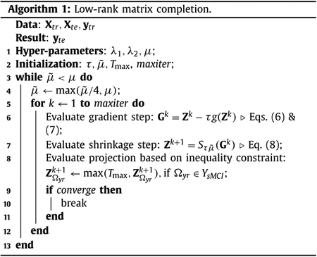
- Gradient step:
where τ is the step size and g (Zk) is the matrix gradient which is defined as(6) (7) - Shrinkage step (Cai et al., 2010):
where S(⋅) is the matrix shrinkage operator, U ΛVT is the SVD of Gk, and max(⋅) is the elementwise maximum operator.(8)
The value of τ is determined from the data. A minor modification of the argument in (Ma et al., 2011; Goldberg et al., 2010) would reveal that, as long as we choose a non-negative step size satisfying τ < min (4|Ωyr|/λ2, 4|Ωyl|/λ1, |Ωχ|), the algorithm above is guaranteed to converge to a global minimum.
4.5. Bayesian hyper-parameter optimization
The problem in Eq. (5) involves multiple hyper-parameters (e.g., μ, λ1, λ2). The values of these hyper-parameters can be obtained by cross-validation and grid search. This is, however, time consuming. For example, if we test 6 candidate values for each hyper-parameter, there would be a total of 63 = 216 combinations. If we test these combinations using 5 fold cross-validation, we will need to solve Eq. (5) more than 1000 times. It is therefore desirable to have a more efficient strategy for the hyper-parameter optimization. In this work, we use a Bayesian optimization algorithm (Bergstra et al., 2011; Thornton et al., 2013; Yogatama and Mann, 2014) to obtain the best hyper-parameters. In this approach, not all the combination of hyper-parameters are tested. Instead, only hyper-parameters that have higher probability of improving the cross-validation accuracy are evaluated. Specifically, Bayesian optimization first builds a prediction model based on previous records of hyper-parameters and their corresponding cross-validation accuracies. Using the prediction model, we obtain the posterior predictive distribution map, which predicts the accuracy distribution for each point in the hyper-parameters search range. Each point in the predictive distribution map can be characterized by a mean and a standard deviation, which are used to denote the prediction accuracy and information gain (the larger the standard deviation, the less certain of the prediction, and the higher of information gain) of this point, respectively. Balancing the information gain and the exploitation of the prediction accuracy, Bayesian optimization arrives at a value via an evaluation function (which is commonly called as acquisition function). Finally, the highest point of the acquisition function is used to choose the hyper-parameter point to be evaluated next. Then the whole process of selecting hyper-parameters is repeated until a stopping criterion is fulfilled.
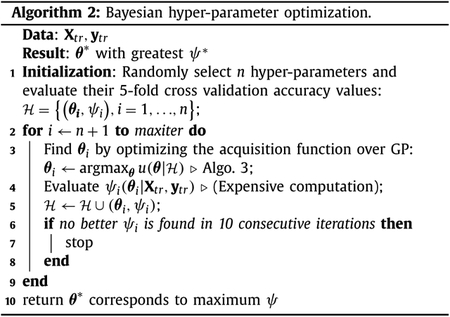
Algorithm 2 outlines the Bayesian optimization method used in this work, called sequential model-based optimization (SMBO) (Bergstra et al., 2011). Let θ denotes a hyper-parameter point, which consists of the hyper-parameters (i.e., μ, λ1, λ2 in (5)) that we need to optimize, ψ denote the corresponding cross validation accuracy using the training data (Xtr, ytr), and denotes the historical observation of the hyper-parameters and their corresponding accuracy values. SMBO performs the following steps iteratively: 1) Build a model that captures the relationship of θ and ψ using a Gaussian process; 2) Determine the next promising θ candidate; 3) Compute ψ based on the selected θ; and 4) Update with a new pair of (θ, ψ) as well as the Gaussian process prediction model.

We solve the problem in line 3 of Algorithm 2 by using a Gaussian Process (GP) prior (Algorithm 3) (Rasmussen, 2004; Rasmussen and Williams, 2006; Bergstra et al., 2011; Thornton et al., 2013; Snoek et al., 2012). GP is an extension of a multivariate Gaussian distribution to an infinite dimensional stochastic process (Brochu et al., 2010). For each θ, ψ(θ) is assumed to be a sample from a multivariate Gaussian distribution, which is completely specified by mean m (θ) and covariance k (θ, θ′):
| (9) |
There are many choices of covariance function (Rasmussen and Williams, 2006; Brochu et al., 2010; Snoek et al., 2012). In this paper, we use the squared exponential covariance function with isotropic distance measure:
| (10) |
where s1 and s2 are the parameters of the covariance function. Assuming that we have historical observation from previous iterations, we want to determine the next plausible hyper-parameter point, θt+1. Let ψt+1 = ψ(θt+1) denotesthe function value at θt+1, and ψ1:t = ψ denotes the column vector of cross validation accuracy values using θ1:t. Then, by the properties of GP, ψ and ψt+1 are jointly Gaussian (Brochu et al., 2010):
| (11) |
where
| (12) |
The parameters s1 and s2 of the covariance function in (10) can be solved by maximizing the probability of ψ given θ (Rasmussen and Williams, 2006):
| (13) |
Based on (11), the posterior predictive distribution is given as (Brochu et al., 2010; Rasmussen and Williams, 2006)
| (14) |
where
| (15) |
| (16) |
Based on the computed mean and covariance function, we evaluate the acquisition function which controls the balance between exploitation (favors θ with higher m) and exploration (favors θ with higher σ2). We use expected improvement (EI) as acquisition function in this study, which is given as (Brochu et al., 2010):
| (17) |
| (18) |
where , and Φ(⋅) ϕ(⋅) are the probability distribution function (PDF) and cumulative distribution function (CDF) of the standard normal distribution, respectively. The hyper-parameter point corresponding to the highest value of the acquisition function is chosen for the next round of hyper-parameter test.
5. Results
We evaluated our proposed framework using both the longitudinal and the multi-modal data. We tested different variations of our proposed framework, and compared them with two baseline methods, as well as two state-of-the-art classification methods that also work on incomplete data. In the following, we describe the baseline methods, the variations of our proposed framework, the state-of-the-art methods, the parameter settings, the performance metrics, and the experimental results.
5.1. The baseline and the proposed methods
One of the differences of our proposed framework with the previous LRMC-based prediction model is the inclusion of LRAD denoising component, which improves the prediction performance significantly. Fig. 2 shows the flowchart of the comparison baseline methods and the proposed methods (i.e., three variations of the proposed framework). For simplicity, we use abbreviations to denote the baseline methods and our proposed methods. The top two rows in Fig. 2, denoted as MC and FMC in the figure, are the baseline methods that do not use LRAD, i.e., LRMC and FS-LRMC (FS-based LRMC), respectively. The following three rows in Fig. 2, denoted as DMC, FDMC and DFMC in the figure, are the proposed methods that utilize LRAD, i.e., LRAD-MC (no feature selection), FS-LRAD-MC (sequentially performing FS, LRAD and LRMC), and LRAD-FS-MC (sequentially performing LRAD, FS and LRMC), respectively. Note that the sequence of applying the feature selection and denoising algorithms will affect the final prediction result. In FS-LRAD-MC, we select features before data denoising, while, in LRAD-FS-MC, we select features after data denoising. While the feature selection algorithm works better if the data is denoised, the denoising algorithm also works better if the data is lower in dimension and discriminative to the prediction task. Therefore, there are pros and cons for both approaches, and we include both models in our study. In the experimental result section, we will discuss a simple guiding principle to help us in deciding which approach to be used in practice.
Fig. 2.

Flow chart of the proposed methods in comparison with the baseline methods. The two baseline methods are LRMC and FS-LRMC, which are respectively abbreviated as MC and FMC. The proposed methods that utilize low-rank affinity pursuit denoising (LRAD) are LRAD-MC, FS-LRAD-MC, and LRAD-FS-MC, which are respectively abbreviated as DMC, FDMC, and DFMC.
5.2. The comparison methods
We compared our method with two state-of-the-art methods – iMSF (Yuan et al., 2012) and Ingalhalikar’s ensemble method (Ingal) (Ingalhalikar et al., 2012). We made some modifications to both algorithms so that they can be applied to our dataset.
1. iMSF:
iMSF is a multi-task learning algorithm where each task is dedicated to the mapping of one data subset to its corresponding target vector. The incomplete dataset is first divided into several disjoint data subsets, each of which is the input for one learning task. The mappings of the subsets to their targets are learned jointly. One of the limitations of this algorithm is the limited number of samples in each disjoint subset. Therefore, we make some modifications to iMSF to use overlapped data subsets for each learning task. This modification greatly increases the number of samples in each data subset, and thus improves the performance of iMSF.
2. Ingalhalikar’s ensemble model (Ingalhalikar et al., 2012):
This algorithm uses an ensemble classification technique to fuse decisions from multiple classifiers constructed using data subsets, obtained similarly as (Thung et al., 2013). The algorithm groups the data into subsets, selects features using signal-to-noise ratio coefficient filter (Guyon and Elisseeff, 2003), performs classification using each data subset based on linear discriminant analysis (LDA), and fuses all classification results into a single result. The decisions are fused using weighted averaging by assigning a weight to the decision of each classifier based on its training classification error. We also implemented a regression ensemble model, where we build a sparse regression model for each data subset and fuse the regression outputs using weighted averaging.
5.3. Hyper-parameters and performance metrics
For our method, we use a small value α = 0.005 for ILRR in (3). The hyper-parameters γ1 and γ2 in feature selection are determined through 5-fold cross validation using only the training data of each fold. The parameters μ, λ1, and λ2 of LRMC are determined using Bayesian optimization as LRMC is more time consuming due to the computation of singular value thresholding. The hyper-parameters of iMSF and Ingalhalikar’s fusion methods are determined using 5-fold cross-validation, since they both involve only one hyper-parameter.
For the classification task involving prediction of diagnostic labels, we use accuracy (ACC) and Area Under the Receiver operator curve (AUC) as the performance metrics. For the regression task involving prediction of MCI conversion time, we choose performance metrics that are less sensitive to the uncertainty or noise in the “ground truth” of conversion time (please refer to Section 3.1), i.e., Pearson correlation coefficient (PCC) and Spearman rank-order correlation coefficient (SROCC). PCC measures the prediction accuracy and SROCC measures the prediction monotonicity. In addition, we also include coefficient determination to measure how well future samples are likely to be predicted by the model. For all the performance metrics, higher values correspond to better predictions.
5.4. Cross-sectional study: prediction of diagnostic labels using multi-modal data and single time point data
Figs. 3 and 4 show respectively the pMCI classification accuracies and AUCs using different combinations of multi-modal data of time point T4 = 18th month. To show the efficacy of each component in the proposed framework, we report the results given by different combinations of the components, i.e., DMC, DFMC and FDMC in Fig. 2, which respectively represents LRAD-MC, FS-LRADMC, and LRAD-FS-MC. LRMC and FS-LRMC, represented by MC and FMC for convenience, are the baseline LRMC methods without LRAD components. More specifically, LRMC and FS-LRMC are the matrix completion algorithms using the original and feature reduced matrices, respectively. Their results are denoted by the blue boxes in Fig. 3. On the other hand, the red boxes in Fig. 3 are used to denote the results of the proposed methods that contain LRAD, i.e.,LRAD-MC, FS-LRAD-MC, and LRAD-FS-MC, represented by DMC, FDMC, and DFMC, respectively.
Fig. 3.

Boxplots of pMCI classification accuracies using different combinations of modalities. MC, FMC, DMC, FDMC, and DFMC denote the abbreviations used for LRMC, FS-LRMC, LRAD-MC, FS-LRAD-MC, and LRAD-FS-MC, respectively (as shown in Fig. 2). Each boxplot summarizes the results of 10 repetitions of 10-fold cross validation. The blue and the red boxes denote the results given by the LRMC without and with the LRAD, respectively. The boxes with darker colors are the results given by the LRMC with feature selection. (For interpretation of the references to color in this figure legend, the reader is referred to the web version of this article.)
Fig. 4.

Boxplots of pMCI classification AUC using different combinations of modalities.
It can be observed from Fig. 3 that the LRAD improves the diagnostic accuracies (i.e., the red boxes are generally higher than the blue boxes). Generally, when LRAD is employed after feature selection, we observe some improvements (comparing FMC with FDMC), especially for MRI+PET, MRI+Cli, and MRI+PET+Cli. In contrast, when feature selection is employed after LRAD, the improvement is not obvious (comparing DMC with DFMC), since using LRAD alone has already significantly improved the accuracy (compare MC with DMC). However, performing feature selection after LRAD can reduce the computation cost because LRMC is applied on a smaller matrix. Similar conclusions can be drawn based on AUC (see Fig. 4).
5.5. Cross-sectional study: influence of regularization
We evaluated the effects of two types of regularization, i.e., the l1 -norm and the l2 -norm, which make different assumptions about the data noise. For the l1 -norm, the data are assumed to be corrupted by sparse noise, which could be caused by any of the preprocessing steps, e.g., segmentation or ROI alignment errors. For the l2 -norm, the data are assumed to be corrupted by Gaussian noise. Tables 2 and 3 show the pMCI/sMCI classification results using multi-modal data of time point T4, with LRAD using an l1 -norm (‖E‖1) or an l2 -norm (‖E‖2) error term. Both tables show that the prediction of LRMC improves with LRAD. We further perform paired t -test between the best result and the other results in each category, and mark the statistically significant results (p < 0.05) with asterisks (*). Comparing the results from both tables, the l1 -norm gives greater improvement than the l2 -norm, implying that the former gives a better denoising outcome.
Table 2.
pMCI classification accuracy using multi-modal data of a single time point (18th month from baseline). An l1 -norm error term is used in ILRR. [Bold: Best result; *: statistically significantly different result compared with the best result (same for all the other Tables in this paper)].
| Data modal | Baseline | ||E||1 in LRR | |||
|---|---|---|---|---|---|
| MC | FMC | DMC | FDMC | DFMC | |
| MRI | 0.686* | 0.706* | 0.726 | 0.715 | 0.720 |
| MRI + PET | 0.686* | 0.700* | 0.724 | 0.737 | 0.726 |
| MRI + Cli | 0.764* | 0.770* | 0.827 | 0.821 | 0.828 |
| MRI + PET + Cli | 0.745* | 0.768* | 0.792 | 0.812 | 0.802 |
Table 3.
pMCI classification accuracy using multi-modal data of a single time point (18th month from baseline). An l2 -norm error term is used in ILRR.
| Modality | Baseline | || E ||2 in LRR | |||
|---|---|---|---|---|---|
| MC | FMC | DMC | FDMC | DFMC | |
| MRI | 0.686* | 0.706 | 0.709 | 0.718 | 0.719 |
| MRI + PET | 0.686* | 0.700* | 0.726 | 0.729 | 0.724 |
| MRI + Cli | 0.764* | 0.770* | 0.808 | 0.807 | 0.809 |
| MRI + PET + Cli | 0.745* | 0.768* | 0.778* | 0.800 | 0.787 |
5.6. Longitudinal study: prediction of diagnostic labels using multi-modal and longitudinal data
Table 4 shows the results using multi-modal and longitudinal data, when the l1 -norm error term is used in LRR. Four time points are used in this experiment, namely time point 1, 2, 3 and 4, corresponding to the data acquired at baseline, 6th month, 12th month, and 18th month, respectively. Time point 4 (T4) is used as our reference time point since it is the latest time point and gives us the most current state of the subject. As shown in our previous work (Thung et al., 2015a, 2015b), predictions using longitudinal data with 2 time points are generally better than using one time point. Hence, we test our method using 2 time points, i.e., the reference time point (T4) plus an additional historical time point data. For example, in Table 4, T4, 1 indicates that the data of T4 and T1 are used. From the table, it can be seen that LRAD improves prediction performance, for almost all combinations of modalities and time-points. The only case where the proposed method performs slightly worse than the baseline is MRI+PET+Cli-T4, 3. The difference is, however, not statistically significant. The highest accuracy achieved by the proposed method is 84.0% for the case of MRI+Cli-T4, 1. Similar observations can be made when the l2 -norm error term is used in LRAD (See Table 5), even though the l1 -norm is generally better than the l2 -norm in this application.
Table 4.
Classification accuracy using longitudinal and multi-modal data. An l1 -norm error term is used in LRAD.
| Modality | Time | Baseline | ||E||1 in LRAD | |||
|---|---|---|---|---|---|---|
| points | MC | FMC | DMC | FDMC | DFMC | |
| MRI | T4 | 0.686* | 0.706* | 0.726 | 0.715 | 0.720 |
| T4,1 | 0.713* | 0.716* | 0.748 | 0.743 | 0.756 | |
| T4,2 | 0.702* | 0.694* | 0.734 | 0.719 | 0.729 | |
| T4,3 | 0.706* | 0.698* | 0.727 | 0.731 | 0.728 | |
| MRI + PET | T4 | 0.686* | 0.700* | 0.724 | 0.737 | 0.726 |
| T4,1 | 0.688* | 0.701* | 0.711 | 0.720 | 0.723 | |
| T4,2 | 0.682* | 0.699 | 0.665* | 0.708 | 0.679* | |
| T4,3 | 0.705 | 0.714 | 0.721 | 0.702 | 0.720 | |
| MRI + Cli | T4 | 0.764* | 0.770* | 0.827 | 0.821 | 0.828 |
| T4,1 | 0.790* | 0.791* | 0.840 | 0.805* | 0.839 | |
| T4,2 | 0.771* | 0.773* | 0.803 | 0.802 | 0.807 | |
| T4,3 | 0.809* | 0.809* | 0.832 | 0.826 | 0.825 | |
| MRI + PET + Cli | T4 | 0.745* | 0.768* | 0.792 | 0.812 | 0.802 |
| T4,1 | 0.765 | 0.760* | 0.753* | 0.777 | 0.755* | |
| T4,2 | 0.730* | 0.759 | 0.736* | 0.767 | 0.757 | |
| T4,3 | 0.788* | 0.808 | 0.789 | 0.796 | 0.800 | |
Table 5.
Classification accuracy using longitudinal and multi-modal data. An l2 -norm error term is used in LRAD.
| Modality | Time | Baseline | ||E||2 in LRAD | |||
|---|---|---|---|---|---|---|
| points | NIC | FMC | DMC | FDMC | DFMC | |
| MRI | T4 | 0.686* | 0.706* | 0.709 | 0.718 | 0.719 |
| T4,1 | 0.713* | 0.716* | 0.734 | 0.738 | 0.740 | |
| T4,2 | 0.702* | 0.694* | 0.723 | 0.725 | 0.723 | |
| T4,3 | 0.706* | 0.698* | 0.716 | 0.728 | 0.726 | |
| MRI + PET | T4 | 0.686* | 0.700* | 0.726 | 0.729 | 0.724 |
| T4,1 | 0.688* | 0.701* | 0.699* | 0.721 | 0.706 | |
| T4,2 | 0.682* | 0.699* | 0.682* | 0.722 | 0.700* | |
| T4,3 | 0.705 | 0.714 | 0.703 | 0.718 | 0.716 | |
| MRI + Cli | T4 | 0.764* | 0.770* | 0.808 | 0.807 | 0.809 |
| T4,1 | 0.790* | 0.791* | 0.820 | 0.800* | 0.821 | |
| T4,2 | 0.771* | 0.773* | 0.798 | 0.790* | 0.802 | |
| T4,3 | 0.809* | 0.809* | 0.822 | 0.826 | 0.816 | |
| MRI + PET + Cli | T4 | 0.745* | 0.768* | 0.778 | 0.800 | 0.787 |
| T4,1 | 0.765 | 0.760* | 0.769 | 0.782 | 0.767 | |
| T4,2 | 0.730* | 0.759 | 0.743* | 0.770 | 0.743* | |
| T4,3 | 0.788* | 0.808 | 0.798 | 0.798 | 0.809 | |
5.7. Cross-sectional study: prediction of conversion time using multi-modal single time point data
Figs. 5 and 6 show respectively the PCC and SROCC results computed between the predicted conversion time and the ground-truth conversion time, using different combinations of multi-modal data of the reference time point. As shown in both figures, the performance of LRMC has been significantly improved with LRAD and feature selection. The best PCC of 0.665, which is about 10% higher than the original LRMC method, is achieved when using MRI data and clinical scores with the proposed framework LRAD-FS-LRMC. Similar results can be observed for coefficient determination (or R2 scores), as shown in Fig. 7.
Fig. 5.

Boxplots of PCC between the predicted and true pMCI conversion times using different combinations of modalities.
Fig. 6.

Boxplots of SROCC between the predicted and true pMCI conversion times using different combinations of modalities.
Fig. 7.

Boxplots of R2 score of pMCI conversion time prediction using different combinations of modalities.
5.8. Longitudinal study: prediction of conversion time using multi-modal and longitudinal data
Table 6 shows the PCC values of the predicted conversion times using different combinations of longitudinal and multi-modal data. As can be seen from the table, the proposed methods (last 2 columns) perform best in all settings. Particularly, for a smaller feature dimension, LRAD-FS-MC (column DFMC) performs better (e.g., MRI, MRI+Cli at T4). For a larger feature dimension, FS-LRADMC (column FDMC) performs better (e.g., MRI+PET, MRI+PET+Cli). The best performance is obtained when using MRI+Cli at T4, which gives us an average PCC value of 0.665. Similar observations can be obtained for SROCC, as shown in Table 7, and R2 scores, as shown in Table 8. Thus, the rule of thumb is to choose LRAD-FS-MC when the feature dimension is smaller and less noisy, and choose FS-LRAD-MC when the feature dimension is bigger and noisier.
Table 6.
PCC of MCI conversion time predictions using longitudinal and multi-modal data. An l1 -norm error term is used in LRR.
| Modality | Time | Baseline | ||E||1 in LRR | |||
|---|---|---|---|---|---|---|
| MC | FMC | DMC | FDMC | DFMC | ||
| MRI | T4 | 0.462* | 0.480* | 0.540* | 0.550 | 0.560 |
| T41 | 0.423* | 0.476* | 0.437* | 0.528 | 0.509 | |
| T42 | 0.440* | 0.459* | 0.451* | 0.524 | 0.504 | |
| T43 | 0.426* | 0.41* | 0.463* | 0.511 | 0.521 | |
| MRI + PET | T4 | 0.512* | 0.531* | 0.454* | 0.568 | 0.550* |
| T41 | 0.415* | 0.502* | 0.448* | 0.533 | 0.512* | |
| T42 | 0.452’ | 0.475* | 0.431* | 0.513 | 0.503 | |
| T43 | 0.442* | 0.485* | 0.467* | 0.522 | 0.491* | |
| MRI + Cli | T4 | 0.566* | 0.594* | 0.643* | 0.639* | 0.665 |
| T41 | 0.552* | 0.582* | 0.605 | 0.587 | 0.607 | |
| T42 | 0.553* | 0.617* | 0.593* | 0.643 | 0.626* | |
| T43 | 0.576* | 0.622 | 0.610 | 0.626 | 0.619 | |
| MRI + PET + Cli | T4 | 0.558* | 0.610* | 0.556* | 0.643 | 0.633 |
| T41 | 0.579* | 0.607 | 0.537* | 0.612 | 0.596* | |
| T42 | 0.471* | 0.598* | 0.569* | 0.616 | 0.621 | |
| T43 | 0.566* | 0.623 | 0.597* | 0.631 | 0.621 | |
Table 7.
SROCC of MCI conversion time predictions using longitudinal and multimodal data. An l1 -norm error term is used in LRR.
| Modality | Time | Baseline | ||E||1 in LRR | |||
|---|---|---|---|---|---|---|
| MC | FMC | DMC | FDMC | DFMC | ||
| MRI | T4 | 0.463 | 0.476 | 0.536 | 0.548 | 0.557 |
| T41 | 0.420 | 0.472 | 0.433 | 0.516 | 0.506 | |
| T42 | 0.440 | 0.457 | 0.446 | 0.523 | 0.506 | |
| T43 | 0.432 | 0.403 | 0.465 | 0.499 | 0.536 | |
| MRI + PET | T4 | 0.492 | 0.524 | 0.446 | 0.554 | 0.551 |
| T41 | 0.400 | 0.498 | 0.444 | 0.514 | 0.506 | |
| T42 | 0.442 | 0.485 | 0.417 | 0.519 | 0.505 | |
| T43 | 0.446 | 0.481 | 0.465 | 0.521 | 0.481 | |
| MRI + Cli | T4 | 0.561 | 0.578 | 0.631 | 0.625 | 0.661 |
| T41 | 0.526 | 0.568 | 0.579 | 0.568 | 0.599 | |
| T42 | 0.543 | 0.605 | 0.593 | 0.635 | 0.613 | |
| T43 | 0.563 | 0.620 | 0.593 | 0.624 | 0.608 | |
| MRI + PET + Cli | T4 | 0.537 | 0.600 | 0.541 | 0.636 | 0.615 |
| T41 | 0.555 | 0.594 | 0.517 | 0.597 | 0.579 | |
| T42 | 0.462 | 0.581 | 0.555 | 0.602 | 0.612 | |
| T43 | 0.566 | 0.613 | 0.591 | 0.622 | 0.609 | |
Table 8.
R2 scores of MCI conversion time predictions using longitudinal and multimodal data. An l1 -norm error term is used in LRR.
| Modality | Time | Baseline | ||E||1 in LRR | |||
|---|---|---|---|---|---|---|
| MC | FMC | DMC | FDMC | DFMC | ||
| MRI | T4 | 0.111 | 0.172 | 0.231 | 0.243 | 0.250 |
| T41 | 0.100 | 0.161 | 0.092 | 0.221 | 0.197 | |
| T42 | 0.1 IS | 0.136 | 0.090 | 0.216 | 0.175 | |
| T43 | 0.094 | 0.104 | 0.100 | 0.201 | 0.208 | |
| MRI + PET | T4 | 0.175 | 0.215 | 0.122 | 0.263 | 0.245 |
| T41 | 0.105 | 0.188 | 0.121 | 0.216 | 0.196 | |
| T42 | 0.124 | 0.144 | 0.117 | 0.208 | 0.182 | |
| T43 | 0.117 | 0.163 | 0.124 | 0.209 | 0.179 | |
| MRI + Cli | T4 | 0.191 | 0.307 | 0.340 | 0.346 | 0.369 |
| T41 | 0.222 | 0.287 | 0.282 | 0.300 | 0.307 | |
| T42 | 0.220 | 0.320 | 0.244 | 0.346 | 0.320 | |
| T43 | 0.239 | 0.325 | 0.270 | 0.325 | 0.321 | |
| MRI + PET + Cli | T4 | 0.190 | 0.308 | 0.224 | 0.344 | 0.336 |
| T41 | 0.261 | 0.294 | 0.209 | 0.312 | 0.292 | |
| T42 | 0.140 | 0.287 | 0.219 | 0.316 | 0.305 | |
| T43 | 0.243 | 0.323 | 0.268 | 0.333 | 0.319 | |
5.9. Discussions
Comparing the results of MRI+PET+Cli and MRI+Cli, especially referring to Table 4, it seems that there is a drop in performance when additional PET data is used. There could be several possible reasons behind this observation, including the small sample size of the data. This is because the number of samples being used is much less than the number of features. The number of samples used in this study is 118, which is relatively small compared to the number of features (93 for each modality at each time point). During training, cross-validation uses an even smaller data subset for feature selection, resulting in instability especially in the presence of outliers and missing data. For the ADNI dataset we used in this study, PET data are not available for half of the samples, whereas clinical cognitive scores and MRI are relatively complete. The relatively smaller number of samples with PET data makes prediction using PET less reliable. We use the results in Table 4 as an example, where columns (c) and (d) refer respectively to our proposed method without and with feature selection. It can be seen that, with feature selection, MRI+PET and MRI+PET+Cli are better than the methods without feature selection, which to some extent verifies our expectation that removing outlier features in the PET data would improve prediction performance.
5.10. Comparison with other methods
In addition, we also compared our method with the methods proposed in (Yuan et al., 2012; Ingalhalikar et al., 2012). Some modifications were made to the method in (Yuan et al., 2012), so that it can be applied to our multi-modal and longitudinal dataset, as described in Section 5.2. The results in Table 9 indicate that the proposed method outperforms these state-of-the-art methods for MRI, MRI+PET and MRI+Cli longitudinal data. For MRI+PET+Cli, the proposed method is still the best when data from a single time point is used, but does not perform as well as iMSF when more time points are used. It is worth noting that this iMSF result is obtained after our improvement modifications, the original iMSF algorithm can not handle so many missing patterns in the longitudinal multi-modal data. Nevertheless, this also likely indicates that a better feature selection method is needed for the proposed framework to further improve performance. As we are focusing on LRAD in this work, we left this as our future work. Similar observation can be obtained for the PCC metric, as shown in Table 10. The best classification and conversion time prediction accuracy for these two tables are still achieved by the proposed LRAD-FS-MC, using MRI and clinical data, at the value of 0.839 and 0.665, respectively.
Table 9.
pMCI classification accuracy using multi-modal and longitudinal data, comparison of results with other methods.
| Modality | Time | iMSF | Ingal | Proposed | ||
|---|---|---|---|---|---|---|
| LogisticR | LeastR | FDMC | DFMC | |||
| MRI | T4 | 0.683 | 0.678 | 0.620 | 0.715 | 0.720 |
| T41 | 0.681 | 0.686 | 0.690 | 0.743 | 0.756 | |
| T42 | 0.690 | 0.694 | 0.643 | 0.719 | 0.729 | |
| T43 | 0.663 | 0.650 | 0.614 | 0.731 | 0.728 | |
| MRI + PET | T4 | 0.687 | 0.684 | 0.680 | 0.737 | 0.726 |
| T41 | 0.658 | 0.654 | 0.721 | 0.720 | 0.723 | |
| T42 | 0.685 | 0.706 | 0.675 | 0.708 | 0.679 | |
| T43 | 0.676 | 0.654 | 0.705 | 0.702 | 0.720 | |
| MRI + Cli | T4 | 0.792 | 0.766 | 0.771 | 0.821 | 0.828 |
| T41 | 0.794 | 0.784 | 0.768 | 0.805 | 0.839 | |
| T42 | 0.800 | 0.789 | 0.772 | 0.802 | 0.807 | |
| T43 | 0.834 | 0.830 | 0.787 | 0.826 | 0.825 | |
| MRI + PET + Cli | T4 | 0.787 | 0.764 | 0.777 | 0.812 | 0.802 |
| T41 | 0.802 | 0.797 | 0.691 | 0.777 | 0.755 | |
| T42 | 0.811 | 0.810 | 0.727 | 0.767 | 0.757 | |
| T43 | 0.832 | 0.806 | 0.717 | 0.796 | 0.800 | |
Table 10.
PCC of pMCI conversion time predictions using multi-modal and longitudinal data, comparison of results with other methods.
| Modality | Time | iMSF | Ingal | Proposed | ||
|---|---|---|---|---|---|---|
| LogisticR | LeastR | FDMC | DFMC | |||
| MRI | T4 | 0.464 | 0.567 | 0.32 | 0.55 | 0.56 |
| T41 | 0.432 | 0.520 | 0.281 | 0.528 | 0.509 | |
| T42 | 0.445 | 0.474 | 0.326 | 0.524 | 0.504 | |
| T43 | 0.397 | 0.493 | 0.307 | 0.511 | 0.521 | |
| MRI + PET | T4 | 0.499 | 0.494 | 0.392 | 0.568 | 0.55 |
| T41 | 0.407 | 0.493 | 0.37 | 0.533 | 0.512 | |
| T42 | 0.502 | 0.507 | 0.364 | 0.513 | 0.503 | |
| T43 | 0.442 | 0.447 | 0.395 | 0.522 | 0.491 | |
| MRI + Cli | T4 | 0.577 | 0.654 | 0.543 | 0.639 | 0.665 |
| T41 | 0.565 | 0.588 | 0.523 | 0.587 | 0.607 | |
| T42 | 0.604 | 0.638 | 0.45 | 0.643 | 0.626 | |
| T43 | 0.653 | 0.651 | 0.48 | 0.626 | 0.619 | |
| MRI + PET + Cli | T4 | 0.578 | 0.621 | 0.491 | 0.643 | 0.633 |
| T41 | 0.621 | 0.584 | 0.429 | 0.612 | 0.596 | |
| T42 | 0.638 | 0.617 | 0.333 | 0.616 | 0.621 | |
| T43 | 0.632 | 0.657 | 0.352 | 0.631 | 0.621 | |
6. Conclusion
In this study, we have proposed a series of algorithms based on subspace methods to address two very important questions on AD study – which MCI subject will progress to AD and when it will occur. Our framework is one of the few studies that addresses these queries jointly using incomplete multi-modal and longitudinal neuroimaging and clinical data. Our framework consists of three main components, i.e., sparse feature selection, low-rank affinity pursuit denoising (LRAD), and low-rank matrix completion (LRMC), in addition to efficient Bayesian hyper-parameter optimization. We have demonstrated that the LRAD is able to improve the LRMC-based predictions, either in terms of the diagnostic labels or the conversion time predictions using MCI data. We use LRAD to denoise heterogeneous multi-modal neuroimaging and clinical data by self-representing the data with the neighboring data. The LRAD with the l1 -norm regularization performs better than the LRAD with the l2 -norm regularization, indicating that the data we used contain more likely sparse noise rather than Gaussian noise. On the other hand, we have modified the original matrix completion algorithm by introducing three data fitting terms and one inequality constraint to predict conversion and time-to-conversion jointly. The added inequality constraint has made the conversion time prediction of the censored sMCI data possible. In addition, we used Bayesian optimization to efficiently search for the optimal set of hyper-parameters for our proposed framework. Extensive evaluations also indicate that the proposed method outperforms the conventional LRMC in various settings, as well as a number of state-of-the-art methods.
Supplementary Material
Acknowledgment
This work was supported in part by NIH grants AG053867, AG041721, AG042599, EB022880, and EB008374. Dr. S.-W. Lee was partially supported by Institute for Information & Communications Technology Promotion (IITP) grant funded by the Korea government (No. 2017-0-00451).
Footnotes
Data used in preparation of this article were obtained from the Alzheimer’s Disease Neuroimaging Initiative (ADNI) database (adni.loni.ucla.edu). As such, the investigators within the ADNI contributed to the design and implementation of ADNI and/or provided data but did not participate in analysis or writing of this report. A complete listing of ADNI investigators can be found at: http://adni.loni.ucla.edu/wp-content/uploads/how_to_apply/ADNI_Acknowledgement_List.pdf.
Supplementary material
Supplementary material associated with this article can be found, in the online version, at 10.1016/j.media.2018.01.002.
References
- Adeli-Mosabbeb E, Thung K-H, An L, Shi F, Shen D, 2015. Robust feature-sample linear discriminant analysis for brain disorders diagnosis. In: Advances in Neural Information Processing Systems, pp. 658–666. [Google Scholar]
- Association A, et al. , 2016. Alzheimer’s disease facts and figures. Alzheimer’s & Dementia 12 (4), 459–509. [DOI] [PubMed] [Google Scholar]
- Association A, et al. , 2017. Alzheimer’s disease facts and figures. Alzheimer’s & Dementia 13 (4), 325–373. [Google Scholar]
- Bergstra JS, Bardenet R, Bengio Y, Kégl B, 2011. Algorithms for hyper-parameter optimization. In: Advances in Neural Information Processing Systems, pp. 2546–2554. [Google Scholar]
- Brochu E, Cora VM, De Freitas N, 2010. A Tutorial on Bayesian Optimization of Expensive Cost Functions, with Application to Active User Modeling and Hierarchical Reinforcement Learning. CoRR; abs/1012.2599. [Google Scholar]
- Cai J-F, Candès EJ, Shen Z, 2010. A singular value thresholding algorithm for matrix completion. SIAM J. Optim 20 (4), 1956–1982. [Google Scholar]
- Cairns NJ, Perrin RJ, Franklin EE, Carter D, Vincent B, Xie M, Bateman RJ, Benzinger T, Friedrichsen K, Brooks WS, et al. , 2015. Neuropathologic assessment of participants in two multi-center longitudinal observational studies: the alzheimer disease neuroimaging initiative (ADNI) and the dominantly inherited alzheimer network (DIAN). Neuropathology 35 (4), 390–400. [DOI] [PMC free article] [PubMed] [Google Scholar]
- Candès EJ, Li X, Ma Y, Wright J, 2011. Robust principal component analysis? J. ACM 58 (3), 11. [Google Scholar]
- Candès EJ, Recht B, 2009. Exact matrix completion via convex optimization. Found. Comput. Math 9 (6), 717–772. [Google Scholar]
- Chen L, Zhang H, Thung K-H, Liu L, Lu J, Wu J, Wang Q, Shen D, 2017. Multi-label inductive matrix completion for joint MGMT and IDH1 status prediction for Glioma patients In: Proceedings of the International Conference on Medical Image Computing and Computer-Assisted Intervention. Springer, pp. 450–458. [DOI] [PMC free article] [PubMed] [Google Scholar]
- Cheng B, Liu M, Suk H-I, Shen D, Zhang D, Initiative ADN, et al. , 2015. Multimodal manifold-regularized transfer learning for MCI conversion prediction. Brain Imaging Behav 9 (4), 913–926. [DOI] [PMC free article] [PubMed] [Google Scholar]
- Cheng B, Liu M, Zhang D, Munsell BC, Shen D, 2015. Domain transfer learning for MCI conversion prediction. IEEE Trans. Biomed. Eng 62 (7), 1805–1817. [DOI] [PMC free article] [PubMed] [Google Scholar]
- Davatzikos C, Bhatt P, Shaw LM, Batmanghelich KN, Trojanowski JQ, 2011. Prediction of MCI to AD conversion, via MRI, CSF biomarkers, and pattern classification. Neurobiol. Aging 32 (12), 2322.e19–2322.e27. [DOI] [PMC free article] [PubMed] [Google Scholar]
- Dukart J, Sambataro F, Bertolino A, 2016. Accurate prediction of conversion to alzheimer’s disease using imaging, genetic, and neuropsychological biomarkers. J. Alzheimers Dis 49 (4), 1143–1159. [DOI] [PubMed] [Google Scholar]
- Elhamifar E, Vidal R, 2011. Sparsity in unions of subspaces for classification and clustering of high-dimensional data In: Proceedings of the 49th Annual Allerton Conference on Communication, Control, and Computing (Allerton). IEEE, pp. 1085–1089. [Google Scholar]
- Elhamifar E, Vidal R, 2013. Sparse subspace clustering: algorithm, theory, and applications. IEEE Trans. Pattern Anal. Mach. Intell 35 (11), 2765–2781. [DOI] [PubMed] [Google Scholar]
- Gauthier S, Reisberg B, Zaudig M, Petersen RC, Ritchie K, Broich K, Belleville S, Brodaty H, Bennett D, Chertkow H, et al. , 2006. Mild cognitive impairment. Lancet 367 (9518), 1262–1270. [DOI] [PubMed] [Google Scholar]
- Goldberg A, Recht B, Xu J, Nowak R, Zhu X, 2010. Transduction with matrix completion: three birds with one stone. Adv. Neural Inf. Process. Syst 23, 757–765. [Google Scholar]
- Guyon I, Elisseeff A, 2003. An introduction to variable and feature selection. J. Mach. Learn. Res 3, 1157–1182. [Google Scholar]
- Huang L, Gao Y, Jin Y, Thung K-H, Shen D, 2015. Soft-split sparse regression based random forest for predicting future clinical scores of Alzheimer’s disease In: Proceedings of the International Workshop on Machine Learning in Medical Imaging Springer, pp. 246–254. [Google Scholar]
- Ingalhalikar M, Parker WA, Bloy L, Roberts TP, Verma R, 2012. Using multi-parametric data with missing features for learning patterns of pathology In: Proceedings of the Medical Image Computing and Computer-Assisted Intervention–MICCAI Springer, pp. 468–475. [DOI] [PMC free article] [PubMed] [Google Scholar]
- Jicha GA, Parisi JE, Dickson DW, Johnson K, Cha R, Ivnik RJ, Tangalos EG, Boeve BF, Knopman DS, Braak H, et al. , 2006. Neuropathologic outcome of mild cognitive impairment following progression to clinical dementia. Arch. Neurol 63 (5), 674–681. [DOI] [PubMed] [Google Scholar]
- Kabani NJ, 1998. A 3d atlas of the human brain. Neuroimage 7, S717. [Google Scholar]
- Korolev IO, Symonds LL, Bozoki AC, Initiative ADN, et al. , 2016. Predicting progression from mild cognitive impairment to alzheimer’s dementia using clinical, MRI, and plasma biomarkers via probabilistic pattern classification. PLoS ONE 11 (2), e0138866. [DOI] [PMC free article] [PubMed] [Google Scholar]
- Li F, Tran L, Thung K-H, Ji S, Shen D, Li J, 2014. Robust deep learning for improved classification of AD/MCI patients In: Proceedings of the International Workshop on Machine Learning in Medical Imaging. Springer, pp. 240–247. [Google Scholar]
- Li F, Tran L, Thung K-H, Ji S, Shen D, Li J, 2015. A robust deep model for improved classification of AD/MCI patients. IEEE J. Biomed. Health Inform 19 (5), 1610–1616. [DOI] [PMC free article] [PubMed] [Google Scholar]
- Lin Y, Chen J, Cao Y, Zhou Y, Zhang L, Tang YY, Wang S, 2015. Unsupervised Cross-Domain Recognition by Identifying Compact Joint Subspaces CoRR; abs/1509.01719. arXiv: 1509.01719. [Google Scholar]
- Lin Y, Chen J, Cao Y, Zhou Y, Zhang L, Wang S, 2015. Cross-domain recognition by identifying compact joint subspaces In: Proceedings of the IEEE International Conference on Image Processing (ICIP) IEEE, pp. 3461–3465. [Google Scholar]
- Liu G, Lin Z, Yan S, Sun J, Yu Y, Ma Y, 2013. Robust recovery of subspace structures by low-rank representation. IEEE Trans. Pattern Anal. Mach. Intell 35 (1), 171–184. [DOI] [PubMed] [Google Scholar]
- Liu G, Lin Z, Yu Y, 2010. Robust subspace segmentation by low-rank representation. In: Proceedings of the 27th International Conference on Machine Learning (ICML-10), pp. 663–670. [Google Scholar]
- Liu G, Yan S, 2011. Latent low-rank representation for subspace segmentation and feature extraction In: Proceedings of the IEEE International Conference on Computer Vision (ICCV) IEEE, pp. 1615–1622. [Google Scholar]
- Liu J, Chen J, Ye J, 2009. Large-scale sparse logistic regression In: Proceedings of the 15th ACM SIGKDD international conference on Knowledge discovery and data mining ACM, pp. 547–556. [Google Scholar]
- Liu J, Ji S, Ye J, 2009b. SLEP: Sparse Learning with Efficient Projections. Arizona State University http://www.public.asu.edu/~jye02/Software/SLEP. [Google Scholar]
- Liu J, Ye J, 2009. Efficient euclidean projections in linear time In: Proceedings of the 26th Annual International Conference on Machine Learning ACM, pp. 657–664. [Google Scholar]
- Liu K, Chen K, Yao L, Guo X, 2017. Prediction of mild cognitive impairment conversion using a combination of independent component analysis and the cox model. Front. Hum. Neurosci 11, 33. [DOI] [PMC free article] [PubMed] [Google Scholar]
- Ma S, Goldfarb D, Chen L, 2011. Fixed point and bregman iterative methods for matrix rank minimization. Math. Program 128 (1–2), 321–353. [Google Scholar]
- Markesbery WR, 2010. Neuropathologic alterations in mild cognitive impairment: a review. J. Alzheimers Dis 19 (1), 221–228. [DOI] [PMC free article] [PubMed] [Google Scholar]
- Michaud TL, Su D, Siahpush M, Murman DL, 2017. The risk of incident mild cognitive impairment and progression to dementia considering mild cognitive impairment subtypes. Dement. Geriatr. Cogn. Dis. Extra 7 (1), 15–29. [DOI] [PMC free article] [PubMed] [Google Scholar]
- Miller RG Jr, 2011. Survival Analysis, 66 John Wiley & Sons. [Google Scholar]
- Misra C, Fan Y, Davatzikos C, 2009. Baseline and longitudinal patterns of brain atrophy in MCI patients, and their use in prediction of short-term conversion to AD: results from ADNI. Neuroimage 44 (4), 1415–1422. [DOI] [PMC free article] [PubMed] [Google Scholar]
- Moradi E, Pepe A, Gaser C, Huttunen H, Tohka J, Initiative ADN, et al. , 2015. Machine learning framework for early MRI-based alzheimer’s conversion prediction in MCI subjects. Neuroimage 104, 398–412. [DOI] [PMC free article] [PubMed] [Google Scholar]
- Nettiksimmons J, DeCarli C, Landau S, Beckett L, 2013. Biological heterogeneity in ADNI amnestic MCI. Alzheimer’s & Dementia J. Alzheimer’s Assoc 4 (9), P222–P223. [DOI] [PMC free article] [PubMed] [Google Scholar]
- Oulhaj A, Wilcock GK, Smith AD, de Jager CA, 2009. Predicting the time of conversion to MCI in the elderly role of verbal expression and learning. Neurology 73 (18), 1436–1442. [DOI] [PMC free article] [PubMed] [Google Scholar]
- Petersen RC, Parisi JE, Dickson DW, Johnson KA, Knopman DS, Boeve BF, Jicha GA, Ivnik RJ, Smith GE, Tangalos EG, et al. , 2006. Neuropathologic features of amnestic mild cognitive impairment. Arch. Neurol 63 (5), 665–672. [DOI] [PubMed] [Google Scholar]
- Rahimi J, Kovacs GG, 2014. Prevalence of mixed pathologies in the aging brain. Alzheimer’s Res. Therapy 6 (9), 82. [DOI] [PMC free article] [PubMed] [Google Scholar]
- Rasmussen CE, 2004. Gaussian Processes in Machine Learning In: Advanced Lectures on Machine Learning Springer, pp. 63–71. [Google Scholar]
- Rasmussen CE, Williams CK, 2006. Gaussian Processes for Machine Learning, 1 MIT press Cambridge. [Google Scholar]
- Sanroma G, Wu G, Gao Y, Thung K-H, Guo Y, Shen D, 2015. A transversal approach for patch-based label fusion via matrix completion. Med. Image Anal 24 (1), 135–148. [DOI] [PMC free article] [PubMed] [Google Scholar]
- Sanroma G, Wu G, Thung K, Guo Y, Shen D, 2014. Novel multi-atlas segmentation by matrix completion In: Proceedings of the International Workshop on Machine Learning in Medical Imaging Springer, pp. 207–214. [Google Scholar]
- She Q, Gan H, Ma Y, Luo Z, Potter T, Zhang Y, 2016. Scale-dependent signal identification in low-dimensional subspace: motor imagery task classification. Neural Plast 2016. [DOI] [PMC free article] [PubMed] [Google Scholar]
- Shen D, Davatzikos C, 2002. HAMMER: Hierarchical attribute matching mechanism for elastic registration. IEEE Trans. Med. Imaging 21 (11), 1421–1439. [DOI] [PubMed] [Google Scholar]
- Shi J, Yang W, Yong L, Zheng X, 2014. Low-rank representation for incomplete data. Math. Probl. Eng 2014. [Google Scholar]
- Sled JG, Zijdenbos AP, Evans AC, 1998. A nonparametric method for automatic correction of intensity nonuniformity in MRI data. IEEE Trans. Med. Imaging 17 (1), 87–97. [DOI] [PubMed] [Google Scholar]
- Snoek J, Larochelle H, Adams RP, 2012. Practical bayesian optimization of machine learning algorithms. In: Advances in Neural Information Processing Systems, pp. 2951–2959. [Google Scholar]
- Stoub T, Bulgakova M, Wilson R, Bennett D, Leurgans S, Wuu J, Turner D, et al. , 2004. MRI-Derived entorhinal volume is a good predictor of conversion from MCI to AD. Neurobiol. Aging 25 (9), 1197–1203. [DOI] [PubMed] [Google Scholar]
- Thornton C, Hutter F, Hoos HH, Leyton-Brown K, 2013. Auto-WEKA: Combined selection and hyperparameter optimization of classification algorithms In: Proceedings of the 19th ACM SIGKDD International Conference on Knowledge Discovery and Data Mining. ACM, pp. 847–855. [Google Scholar]
- Thung K-H, Adeli E, Yap P-T, Shen D, 2016. Stability-weighted matrix completion of incomplete multi-modal data for disease diagnosis In: Proceedings of the International Conference on Medical Image Computing and Computer-Assisted Intervention Springer, pp. 88–96. [DOI] [PMC free article] [PubMed] [Google Scholar]
- Thung K-H, Wee C-Y, Yap P-T, Shen D, 2013. Identification of Alzheimer’s disease using incomplete multimodal dataset via matrix shrinkage and completion In: Proceedings of the International Workshop on Machine Learning in Medical Imaging Springer, pp. 163–170. [Google Scholar]
- Thung K-H, Wee C-Y, Yap P-T, Shen D, 2014. Neurodegenerative disease diagnosis using incomplete multi-modality data via matrix shrinkage and completion. Neuroimage 91, 386–400. [DOI] [PMC free article] [PubMed] [Google Scholar]
- Thung K-H, Wee C-Y, Yap P-T, Shen D, 2016. Identification of progressive mild cognitive impairment patients using incomplete longitudinal MRI scans. Brain Struct. Funct 221 (8), 3979–3995. [DOI] [PMC free article] [PubMed] [Google Scholar]
- Thung K-H, Yap P-T, Adeli-M E, Shen D, 2015. Joint diagnosis and conversion time prediction of progressive mild cognitive impairment (pmci) using low-rank subspace clustering and matrix completion In: Proceedings of the Medical Image Computing and Computer-Assisted Intervention - MICCAI. Springer, pp. 527–534. [DOI] [PMC free article] [PubMed] [Google Scholar]
- Thung K-H, Yap P-T, Shen D, 2017. Multi-stage diagnosis of Alzheimer’s disease with incomplete multimodal data via multi-task deep learning In: Deep Learning in Medical Image Analysis and Multimodal Learning for Clinical Decision Support. Springer, pp. 160–168. [DOI] [PMC free article] [PubMed] [Google Scholar]
- Tibshirani R, 1996. Regression shrinkage and selection via the lasso. J. R. Stat. Soc. Ser. B Methodol 267–288. [Google Scholar]
- Troyanskaya O, Cantor M, Sherlock G, Brown P, Hastie T, Tibshirani R, Botstein D, Altman RB, 2001. Missing value estimation methods for DNA microarrays. Bioinformatics 17 (6), 520–525. [DOI] [PubMed] [Google Scholar]
- Vidal R, 2010. A tutorial on subspace clustering. IEEE Signal Process. Mag 28 (2), 52–68. [Google Scholar]
- Wang Y, Nie J, Yap P-T, Shi F, Guo L, Shen D, 2011. Robust deformable-surface-based skull-stripping for large-scale studies. Medical Image Computing and Computer-Assisted Intervention–MICCAI 2011 635–642. [DOI] [PubMed] [Google Scholar]
- Wei R, Li C, Fogelson N, Li L, 2016. Prediction of conversion from mild cognitive impairment to Alzheimer’s disease using MRI and structural network features. Front. Aging Neurosci 8, 76. [DOI] [PMC free article] [PubMed] [Google Scholar]
- Weiner MW, Veitch DP, Aisen PS, Beckett LA, Cairns NJ, Green RC, Harvey D, Jack CR, Jagust W, Liu E, et al. , 2013. The alzheimer’s disease neuroimaging initiative: a review of papers published since its inception. Alzheimer’s Dementia 9 (5), e111–e194. [DOI] [PMC free article] [PubMed] [Google Scholar]
- Wright J, Ganesh A, Rao S, Peng Y, Ma Y, 2009. Robust principal component analysis: Exact recovery of corrupted low-rank matrices via convex optimization. In: Advances in Neural Information Processing Systems, pp. 2080–2088. [Google Scholar]
- Xiang S, Yuan L, Fan W, Wang Y, Thompson PM, Ye J, Initiative ADN, et al. , 2014. Bi-level multi-source learning for heterogeneous block-wise missing data. Neuroimage 102, 192–206. [DOI] [PMC free article] [PubMed] [Google Scholar]
- Xu L, Wu X, Li R, Chen K, Long Z, Zhang J, Guo X, Yao L, 2016. Prediction of progressive mild cognitive impairment by multi-modal neuroimaging biomarkers. J. Alzheimers Dis 51 (4), 1045–1056. [DOI] [PubMed] [Google Scholar]
- Xue Z, Shen D, Davatzikos C, 2004. Determining correspondence in 3-d MR brain images using attribute vectors as morphological signatures of voxels. IEEE Trans. Med. Imaging 23 (10), 1276–1291. [DOI] [PubMed] [Google Scholar]
- Xue Z, Shen D, Davatzikos C, 2006. Statistical representation of high-dimensional deformation fields with application to statistically constrained 3D warping. Med. Image Anal 10 (5), 740–751. [DOI] [PubMed] [Google Scholar]
- Xue Z, Shen D, Karacali B, Stern J, Rottenberg D, Davatzikos C, 2006. Simulating deformations of MR brain images for validation of atlas-based segmentation and registration algorithms. Neuroimage 33 (3), 855–866. [DOI] [PMC free article] [PubMed] [Google Scholar]
- Yogatama D, Mann G, 2014. Efficient Transfer Learning Method for Automatic Hyperparameter Tuning In: Kaski S, Corander J (Eds.), Proceedings of the Seventeenth International Conference on Artificial Intelligence and Statistics, 33. PMLR, Reykjavik, Iceland, pp. 1077–1085 Proceedings of Machine Learning Research. [Google Scholar]
- Yu G, Liu Y, Thung K-H, Shen D, 2014. Multi-task linear programming discriminant analysis for the identification of progressive MCI individuals. PLoS ONE 9 (5), e96458. [DOI] [PMC free article] [PubMed] [Google Scholar]
- Yuan L, Wang Y, Thompson PM, Narayan VA, Ye J, Initiative ADN, et al. , 2012. Multi-source feature learning for joint analysis of incomplete multiple heterogeneous neuroimaging data. Neuroimage 61 (3), 622–632. [DOI] [PMC free article] [PubMed] [Google Scholar]
- Zhan L, Zhou J, Wang Y, Jin Y, Jahanshad N, Prasad G, Nir TM, Leonardo CD, Ye J, Thompson PM, et al. , 2015. Comparison of nine tractography algorithms for detecting abnormal structural brain networks in Alzheimer’s disease. Front Aging Neurosci 7. [DOI] [PMC free article] [PubMed] [Google Scholar]
- Zhang D, Shen D, Initiative ADN, et al. , 2012. Multi-modal multi-task learning for joint prediction of multiple regression and classification variables in alzheimer’s disease. Neuroimage 59 (2), 895–907. [DOI] [PMC free article] [PubMed] [Google Scholar]
- Zhang Y, Brady M, Smith S, 2001. Segmentation of brain MR images through a hidden Markov random field model and the expectation-maximization algorithm. IEEE Trans. Med. Imaging 20 (1), 45–57. [DOI] [PubMed] [Google Scholar]
- Zhou T, Thung K-H, Zhu X, Shen D, 2017. Feature learning and fusion of multimodality neuroimaging and genetic data for multi-status dementia diagnosis In: Proceedings of the International Workshop on Machine Learning in Medical Imaging Springer, pp. 132–140. [DOI] [PMC free article] [PubMed] [Google Scholar]
- Zhou X, Yang C, Yu W, 2013. Moving object detection by detecting contiguous outliers in the low-rank representation. Pattern Anal. Mach. Intell. IEEE Trans 35 (3), 597–610. [DOI] [PubMed] [Google Scholar]
- Zhu X, Suk H-I, Thung K-H, Zhu Y, Wu G, Shen D, 2016. Joint discriminative and representative feature selection for Alzheimer’s disease diagnosis In: Proceedings of the International Workshop on Machine Learning in Medical Imaging Springer, pp. 77–85. [DOI] [PMC free article] [PubMed] [Google Scholar]
- Zhu X, Suk H-I, Zhu Y, Thung K-H, Wu G, Shen D, 2015. Multi-view classification for identification of Alzheimer’s disease In: Proceedings of the International Workshop on Machine Learning in Medical Imaging. Springer, pp. 255–262. [DOI] [PMC free article] [PubMed] [Google Scholar]
- Zhu X, Thung K-H, Adeli E, Zhang Y, Shen D, 2017. Maximum mean discrepancy based multiple kernel learning for incomplete multimodality neuroimaging data In: Proceedings of the International Conference on Medical Image Computing and Computer-Assisted Intervention Springer, pp. 72–80. [DOI] [PMC free article] [PubMed] [Google Scholar]
- Zhu X, Zhang S, Jin Z, Zhang Z, Xu Z, 2011. Missing value estimation for mixed-attribute data sets. IEEE Trans. Knowl. Data Eng 23 (1), 110–121. [Google Scholar]
Associated Data
This section collects any data citations, data availability statements, or supplementary materials included in this article.