

Abstract
Purpose
To develop an efficient algorithm for multi‐component analysis of magnetic resonance fingerprinting (MRF) data without making a priori assumptions about the exact number of tissues or their relaxation properties.
Methods
Different tissues or components within a voxel are potentially separable in MRF because of their distinct signal evolutions. The observed signal evolution in each voxel can be described as a linear combination of the signals for each component with a non‐negative weight. An assumption that only a small number of components are present in the measured field of view is usually imposed in the interpretation of multi‐component data. In this work, a joint sparsity constraint is introduced to utilize this additional prior knowledge in the multi‐component analysis of MRF data. A new algorithm combining joint sparsity and non‐negativity constraints is proposed and compared to state‐of‐the‐art multi‐component MRF approaches in simulations and brain MRF scans of 11 healthy volunteers.
Results
Simulations and in vivo measurements show reduced noise in the estimated tissue fraction maps compared to previously proposed methods. Applying the proposed algorithm to the brain data resulted in 4 or 5 components, which could be attributed to different brain structures, consistent with previous multi‐component MRF publications.
Conclusions
The proposed algorithm is faster than previously proposed methods for multi‐component MRF and the simulations suggest improved accuracy and precision of the estimated weights. The results are easier to interpret compared to voxel‐wise methods, which combined with the improved speed is an important step toward clinical evaluation of multi‐component MRF.
Keywords: joint sparsity constraint, MR fingerprinting, multi‐component analysis, NNLS, partial volume effect, Sparsity Promoting Iterative Joint NNLS (SPIJN)
1. INTRODUCTION
Magnetic resonance fingerprinting (MRF)1 is a novel technique for simultaneous mapping of multiple quantitative parameters. MRF has been mainly applied for single‐component matching of a set of system and tissue parameters, e.g. , , and , to each voxel. The standard method matches the measured signal to a pre‐calculated dictionary with a pattern recognition algorithm based on the inner product similarity measure. However, single‐component matching only considers the average signal produced by multiple tissues in a voxel. Multiple tissues can be present in a voxel either in the boundary region between 2 tissues or simply as a mixture of multiple components because of the complex structure of tissue. In the brain, the first effect occurs in the boundary region between white and gray matter, the second example is the case for myelin in the white matter. This partial volume effect2 can lead to blurring artifacts or averaged tissue parameters in the maps obtained by single component matching.
Multi‐component analysis takes into account that a voxel can consist of several tissues and assumes that the measured signal is composed of a weighted sum of signals corresponding to the individual tissues present in the voxel. Multi‐component analysis can be performed for standard relaxometry scans like multi‐echo spin echo (MESE) mapping by a multi‐exponential fit. The standard method for multi‐component analysis is the T2 Non‐Negative Least Squares (T2NNLS) algorithm introduced by Whittall and MacKay,3 based on the Non‐Negative Least Squares (NNLS) algorithm by Lawson and Hanson.4 With this algorithm a smooth spectrum is obtained and the Myelin Water Fraction (MWF) is determined by integrating over all weights in the spectrum with ms. Besides myelin water, another peak can be recognized which belongs to intra‐extracellular water.5
Multi‐component analysis applied to MRF has the potential to distinguish more tissues than multi‐exponential methods because multiple tissue parameters are taken into account. A first approach to Multi‐Component MRF (MC‐MRF), where each voxel is modeled as a composition of only 3 possible tissues with predefined relaxation times, was proposed in the supplemental material of the original MRF publication.1 A dictionary containing only 3 , combinations was used with a least‐squares algorithm to determine the weights for the 3 possible components. This approach imposes a very strong constraint, namely that the number and relaxation times of the individual components are known. This may not always be the case and the resulting solution is very sensitive to the choice of tissue parameters. Deshmane et al6 expanded this approach by estimating the main tissues based on the single component matching combined with k‐means clustering, where the number of components is selected on forehand. This partial volume model assumes that most voxels contain a single component and partial volume effects are only present at the boundaries of tissues (See Supporting Information Figure S1). A first MC‐MRF method using a large dictionary of and combinations was proposed by McGivney et al7 which applies a Bayesian estimation method to obtain a MC‐MRF matching. This method considers each voxel independently and is able to distinguish different components within a voxel without explicitly including prior knowledge about the number of components or their corresponding relaxation times. This approach applies a sparsity constraint, but the coefficient weights are complex and the absolute value of the complex weights is returned as the final solution. Computation times of 12 s per voxel were reported in this work, corresponding to several days for the processing of a single slice. Another voxel‐wise approach was recently proposed by Tang et al8 which applies both sparsity and non‐negativity constraints to the component weights within an iteratively reweighted ‐norm regularized least squares algorithm. Computation times between 0.1 s and 1 s for a single voxel are reported for this algorithm when executed on a computer cluster.
Besides the long processing times reported in these approaches, another difficulty is the interpretation and visualization of the results. When the complete MRF measurement is considered, the matched components in each voxel can correspond to different relaxation times, and need further processing to visualize the results. This can be done with a simple grouping based on or ranges as done for the MWF from T2NNLS or with a more sophisticated method, e.g. Bayesian grouping strategies.9 This interpretation step requires additional assumptions about the tissues present in the region of interest (ROI), the number of components or voxels in which a pure tissue can be found.
Two works are currently published in arXiv, in which the multi‐component analysis includes dependencies between different voxels. The greedy‐approximate projection algorithm (GAP‐MRF)10 approximates the main tissues present in the ROI and determines MC‐MRF maps based on these components. This method results in 5‐6 components in the brain, assuming that most voxels contain single tissue. Relaxation‐Relaxation Correlation Spectroscopic Imaging (RR‐CSI)11 is a related approach, which uses an inversion recovery multi‐echo spin‐echo (IR‐MESE) acquisition sequence simultaneously encoding and relaxation times. The corresponding multi‐component analysis assumes smoothness in the parameter space and spatial smoothness to determine distributions for all voxels. This method can be seen as an extension on T2NNLS methods where spatial smoothness is applied12, 13, 14 and multiple relaxation parameters are simultaneously encoded. Six main peaks are detected in the reconstructed spectrum, which are interpreted as 6 different components. This algorithm was not demonstrated on MRF‐data, but is related because it performs multi‐component analysis from a sequence simultaneously encoding and relaxation times. Another work by the same authors proposes a set of greedy algorithms for non‐negativity constraining simultaneous sparse recovery,15 related to the GAP‐MRF algorithm.10
In this study, we investigate different approaches for MC‐MRF with the aim to obtain an accurate and robust result in a shorter time than the previously proposed MC‐MRF approaches. Several different approaches were implemented and compared, including the NNLS algorithm as used for T2NNLS, the fixed 3 component approach presented in the original MRF publication,1 the Bayesian algorithm7 and reweighted‐‐norm regularized algorithm.8 Furthermore, we propose a new algorithm that applies joint sparsity and non‐negativity constraints for the component weights, which can reduce the noise amplification in MC‐MRF keeping the reconstruction time tractable. The main premise of this approach is that only a small number of “basis” tissues is present throughout the ROI and the tissue in each voxel is a mixture of these basis tissues. The method is theoretically described and compared with the previously mentioned methods. The evaluation was performed in numerical simulations and in brain data of 11 healthy volunteers.
2. METHODS
2.1. Theory
2.1.1. Voxel‐wise problem setting
In a multi‐component signal model, the MRF signal of a voxel j ∈ {1, 2, … J}, where J is the number of voxels, can be written as
| (1) |
where D is the MRF dictionary, the vector containing the weights for the different components and the noise term. The measured MRF signal is generally complex, however, if the phase is known, the signal can be rotated to the real axis resulting in a real vector of length M, where M is the number of time points of the fingerprinting sequence or the length of the signal after SVD compression.16
The dictionary contains the signal evolutions for N different components. The measured signal is modeled as a non‐negative linear combination of the dictionary signals. The weights of these different components are contained in the vector . Besides the non‐negativity constraint, it can be assumed that the weight vector is sparse, thus the measured signal can be represented by a small number of components, representing a small number of tissue types. The weights for each component in Equation (1) can be obtained by least squares minimization. When we include the requirement that c is non‐negative, we obtain the following NNLS problem for each voxel j:
| (2) |
For a dictionary with a large number of components, this problem is highly under‐determined and has infinitely many solutions. This formulation is very similar to a compressed sensing problem. Therefore, if the solution vector is sparse, there are some theoretical guarantees that it can be recovered using a sparsity constraint. However, due to the high coherence of MRF dictionaries a unique solution only exists for very sparse solutions. One sparsity promoting approach to solve this problem is the active set NNLS algorithm as proposed by Lawson and Hanson4 [Chapter 23]. The NNLS algorithm shows similarities to the orthogonal matching pursuit (OMP) algorithm17 with its active set principle and results in sparse solutions.
Another approach to restrict the solution is in the form of regularization. A typical choice for sparsity promoting regularization is the ‐norm. The non‐negativity constraint makes it possible to use the ‐non‐negative regularization instead, which can be used with computationally more efficient algorithms18:
| (3) |
where λ > 0 is the regularization parameter. This problem can be recast to the equivalent non‐negative least squares problem of the form
| (4) |
where and are given by:
| (5) |
which can still be solved using the NNLS algorithm from.4 In this setting, an independent (sparse) solution is obtained for each voxel.
2.1.2. Joint sparsity constraint
The voxel‐wise approach can lead to different components for each voxel, even for a small region of interest that has uniform intensity in a contrast weighted image. This is most likely due to noise and not due to actual large variability in the tissue composition. The main premise in this work is that the tissue in the measured volume is composed of a small number of “basis tissues,” or components, which are shared for all voxels in the region of interest. In other words, we assume that there is a small number of dictionary signals (atoms), which form a basis for the measured MRF signal for the whole region of interest. The measured MRF signals can be represented by a linear combination of this shared set of dictionary signals. This assumption is similar to the fixed basis approach,1 however, we don't assume that the number of components and their and values are known in advance. To include this requirement in the reconstruction, we introduce the joint sparsity constraint.
The joint forward model can be written as
| (6) |
where contains the measured signals and contains the weights for all the voxels and E contains the noise terms. Each row of the weight matrix contains the weights of a single component i for all voxels in the region of interest. The joint inverse problem can be written as a NNLS minimization problem:
| (7) |
where denotes the Frobenius norm.
The requirement that the measured signals can be represented by a small number of shared signals, can be summarized as the constraint that must be small. This joint sparsity constraint has been considered with different names and in different problem settings19, 20, 21, 22, 23 and has only been combined with a non‐negativity constraint in a Greedy algorithm.15 The non‐negativity and joint sparsity constraints can be combined in the minimization problem
| (8) |
where μ is a regularization parameter that balances sparsity and reconstruction error.
2.1.3. Sparsity promoting iterative joint non‐negative least squares (SPIJN) algorithm
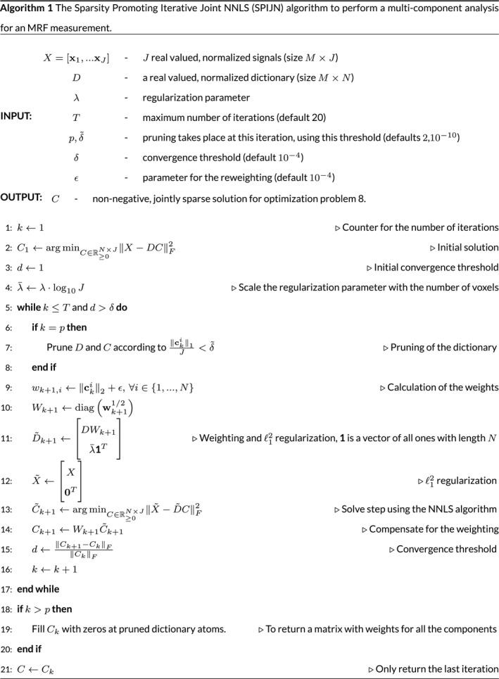
To solve the optimization problem 8, we propose a new iteratively reweighted non‐negative least squares algorithm, called Sparsity Promoting Iterative Joint NNLS (SPIJN), which is summarized in Algorithm 1 to which we will refer in the rest of this section. In the spirit of reproducible research, the source code of the proposed algorithm including the later discussed numerical phantom is available at https://github.com/MNagtegaal/SPIJN. The algorithm uses the NNLS algorithm to solve the joint NNLS problem, with a reweighting in each iteration. The weights promote a jointly sparse solution, finding a small number of atoms that serve as a common basis for all voxels. Both the measured signals X and the dictionary D are normalized such that . The normalization of the dictionary prevents a bias caused by high signal intensity, the normalization of the signals makes sure that all voxels have an equal influence on the joint sparsity.
The core of the algorithm is formed by lines 9‐14. In each iteration, the NNLS algorithm is used to solve the reweighted problem in line 13. The weights
| (9) |
are used, where ε is a small parameter to improve the stability. To make the reweighting more effective, the regularization from Equation (5) is used in lines 11 and 12 of the algorithm. The regularization parameter λ is scaled with , to make the values of the regularization parameter less sensitive to the number of voxels. The scaled regularization parameter determines the sparsity of the solution, similar to μ in Equation (8). The algorithm is stopped after T iterations or when convergence is reached, according to
| (10) |
where δ is the convergence threshold, as calculated in line 15.
Most of the dictionary elements are not used after a small number of iterations and remain unused for the rest of the process. These dictionary elements can therefore be removed from the dictionary (line 7) to speed up the computations. This pruning is performed in iteration p, where rows with an norm smaller than are pruned. In the final solution, the weights corresponding to the pruned dictionary atoms are set to 0.
2.2. Experiments
2.2.1. Simulated data
To test the proposed method, simulations were performed with a fully sampled numerical phantom containing 3 different components. The relaxation times for the simulated components were chosen according to a 3 tissue brain model, where the measured MR signal is a combination of myelin water (MW), intra‐ and extracellular water (IEW) and free water (FW). The first component is in the range of MW with relaxation times ( ms and ) ms,24 the second component in the range IEW ( ms and ms) and the third component in the range of FW ( ms and ms).25 multi‐component compositions were simulated, the first component had a weight of 10% in each composition, the other 2 components vary from 0% to 90%. For each combination, the signal evolution was calculated and Gaussian noise was added, resulting in a total of 10 × 10 simulated voxels with a signal to noise ratio of 50. A gradient‐spoiled MRF sequence26 of 200 time points was used for the simulations. The sequence had a flip angle variation as shown in Figure 1 (Sequence 1) and a constant repetition time of TR = 15 ms.
Figure 1.
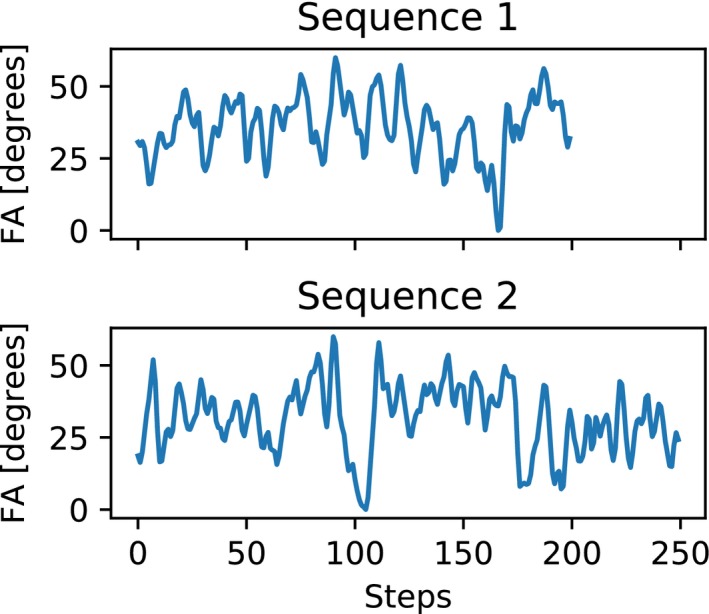
The 2 flip angle (FA) sequences used in this work. Both sequences have a repetition time of 15 ms. Sequence 1 has a TE = 4 ms and repetition delay of 500 ms. Sequence 2 has a TE = 5 ms and repetition delay of 3 s. The maximal flip angle in both sequences is 60
A logarithmically spaced dictionary with 3240 atoms consisting of 80 values from 10 ms to 5 s and 80 values from 10 ms to 5 s with the restriction was computed with the extended phase graph algorithm (EPG).27
2.2.2. In vivo data
To demonstrate the feasibility of the proposed method in vivo, fully sampled MRF brain data were acquired for 11 healthy volunteers with informed consent obtained. The scans were performed with different MRF sequences on 2 different field strengths in order to test the approach in different settings. The measured signals were corrected with a phase term to obtain real‐valued vectors. In a pre‐processing step, the lipid tissue and skin were removed to keep only the region containing the brain.
One volunteer scan was performed on a 1.5 T Philips Achieva scanner with Sequence 1 as given in Figure 1 using an 8 channel head coil and a spiral acquisition pattern, a FOV of 240 × 240 , 1 × 1 in plane resolution and 5 mm slice thickness. Three slices were acquired with an acquisition time of 359 s. A logarithmically spaced dictionary was computed with ranging from 10 ms to 4 s in 100 steps and from 4 ms to 2 s in 80 steps, with the restriction , consisting of 4974 dictionary atoms.
Ten volunteers were scanned on a 3.0 T Philips Ingenia scanner with Sequence 2 as given in Figure 1 with a Cartesian sampling pattern, a FOV of 240 × 240 , in plane resolution of 1.25 × 1.25 and 10 mm slice thickness. The acquisition time for 1 slice was 337 s. For the dictionary the same and combinations were used as in the numerical experiments and included different relative ‐inhomogeneity values, ranging from 0.75 to 1.26 with step size 0.003, leading to a dictionary size of 845580.
2.2.3. Comparison to other algorithms
The proposed SPIJN algorithm was compared in simulations to 3 voxel‐wise algorithms, the NNLS algorithm,4 the MC‐MRF reweighted‐‐norm regularized algorithm8 and the MC‐MRF Bayesian approach.7 The NNLS forms the basis of our algorithm and a comparison is included in order to estimate the effects of the joint sparsity constraint. The 1.5 T measurement was used to compare the SPIJN algorithm to the 3 voxel‐wise algorithms and MC‐MRF analysis using 2 different subdictionaries containing only 3 fixed components. The first set (set A) of components of the subdictionaries is based on literature values from a work applying this approach for MC‐MRF28 and the (, ) values are (127 ms, 21 ms), (1267 ms, 127 ms) and (2056 ms, 485 ms). The second set B is based on components as matched by SPIJN with (, ) relaxation times (10 ms, 10 ms), (781 ms, 58 ms) and (1821 ms, 842 ms). The comparison with the 2 different sets of fixed components was performed to evaluate the sensitivity to the choice of the components. The normalized root mean squared error (NRMSE) is used to evaluate the data consistency between the estimated signal from the multi‐component matching and the measured signal. The NRMSE is calculated as .
For the Bayesian algorithm 3 parameters had to be chosen, for the shape parameters α = 2 and β = 0.1 were used. Regularization parameter μ = 6 was used for the in vivo measurement and μ = 0.01 for the simulations. For the reweighted‐‐norm regularized algorithm λ = 0.01 was used for the in vivo data and λ = 0.001 for the simulations. For the SPIJN algorithm λ = 3.5 was used for the 1.5 T in vivo measurements and λ = 0.03 in the simulations.
All algorithms were implemented in Python. SVD compression16 to a dimension of 25 was used for all the measurements and simulations. The NNLS algorithm uses the FORTRAN implementation as included in the SciPy package. For the subdictionaries the NNLS algorithm was used to find the corresponding weights for the fixed components.
The single‐voxel algorithms require grouping to relate similar components found in different voxels to each other and to known tissue types. Components in the range and are considered to belong to the MW component, in the range and to the IEW and in the range and to the FW. Components outside these ranges are considered as outliers and not grouped to any of the 3 water types. These ranges are based on a combination of the following; relaxation times as expected from literature,29 ranges as used for relaxometry MWF mapping and the visually distinguishable clusters in the MC‐MRF decompositions from the different algorithms.
2.2.4. Repeatability of the SPIJN algorithm
The 10 MRF measurements at 3 T were used to evaluate the repeatability of the multi‐component matching from the SPIJN algorithm on multiple healthy volunteers with the same MRF sequence. Single component matching was first used to obtain the map. Then for each voxel the corresponding subdictionary with fixed , was selected for the MC‐MRF analysis. The SPIJN algorithm was then used to obtain a decomposition for each of the measurements. The regularization parameter was selected in a way that the number of components was as small as possible but without increasing the NRMSE compared to regularized voxel‐wise methods. This resulted in λ values of either 12 or 15 for these measurements. From these decompositions, the components corresponding to white and gray matter were selected for the evaluation.
The relaxation times matched to the white and gray matter are determined as an indication of the repeatability of the SPIJN decomposition over multiple scans. An overview of relaxation times for white and gray matter at 3 T from different studies25, 29 is given in Table 1 as a reference.
Table 1.
| Average (ms) | Std (ms) | Min (ms) | Max (ms) | # Studies | ||
|---|---|---|---|---|---|---|
|
|
||||||
| Gray matter | 1459 | 192.3 | 968 | 1815 | 20 | |
| White matter | 974 | 210 | 728 | 1735 | 26 | |
|
|
||||||
| Gray matter | 92.6 | 16.9 | 65 | 110 | 5 | |
| White matter | 60.8 | 13.1 | 49.5 | 79.6 | 4 |
The tables include the number of studies resulting in the list of literature values used to determine the average values, standard deviations, and minimal and maximal values.
3. RESULTS
3.1. Comparison to other algorithms
3.1.1. Simulated data
The results of the multi‐component analysis for the simulated data are shown in Figures 2 and 3. Figure 2 shows the ground truth of the 3 different components and the component weights obtained by the 4 different algorithms. The root mean squared error (RMSE) is given above each of the grouped components. The results of the NNLS and the reweighted‐‐norm‐regularized algorithm are very similar, while the Bayesian approach results in larger errors than the other 2 voxel‐wise methods. The SPIJN algorithm results in a smaller error and less variance in the solution.
Figure 2.
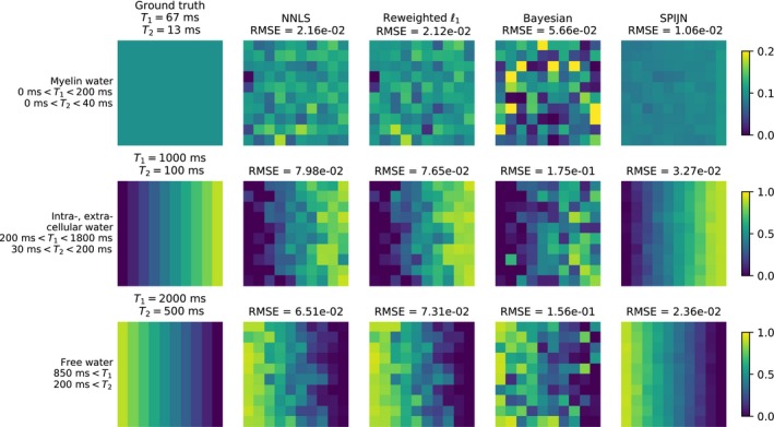
The results of the simulations with 3 components comparing the 4 different MC‐MRF algorithms. Sequence 1 as shown in Figure 1 was used in the simulation. A numerical phantom containing 3 different components was simulated with an SNR of 50. The numerical phantom consists of 100 pixels, the first component is present in each pixel with 10% and the other two components vary in the horizontal direction from 0 to 90% in 10 steps. The first column shows the ground truth for the distribution of the weights for the different components and the other columns show the retrieved component weights with the different algorithms and the corresponding root mean squared error (RMSE) to the ground truth
Figure 3.
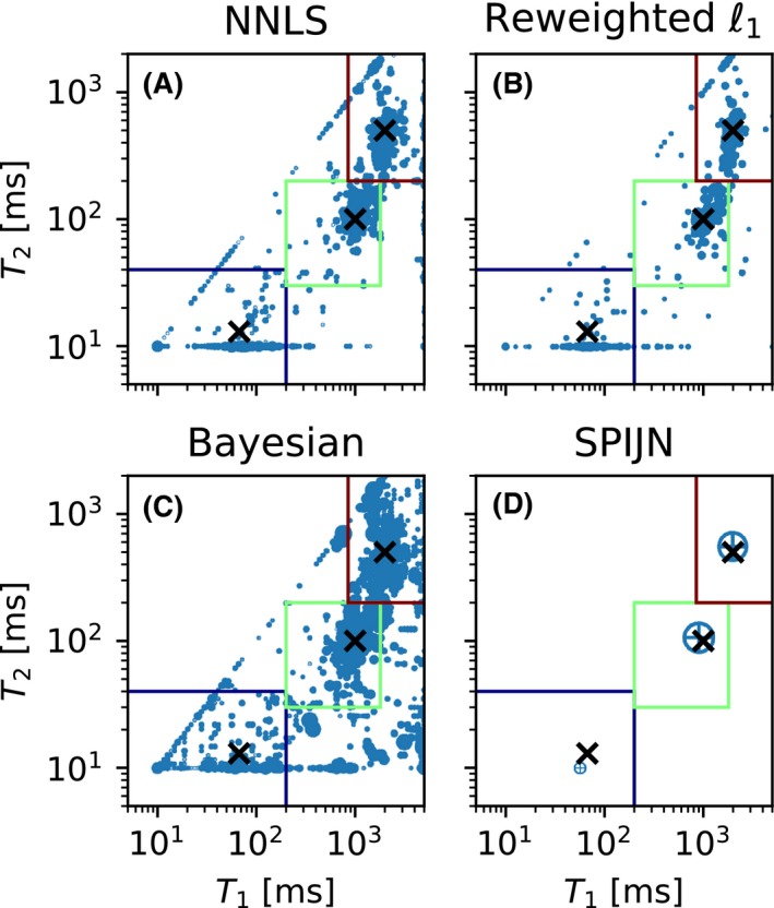
The distribution of the matched components for the numerical phantom with the different algorithms. The boxes indicate how the components are grouped. The blue box is the short component, the green box the middle component and the red box the long component. The size of the circles corresponds to the relative abundance of the components. The 3 crosses give the locations of the true components
Figure 3 shows the distribution of the and values of the matched components for the different algorithms, the grouping boxes and the true relaxation times of the simulated components. The matched components are spread around the true relaxation times and for all the algorithms the component with the shortest and is the most difficult to estimate. Although the and values of the shortest component are biased, the corresponding component weights are still accurate.
The reweighted‐‐norm regularized algorithm shows a smaller spread in the relaxation times of the matched components compared to the other voxel‐wise methods, but the differences with the NNLS algorithm are small. The SPIJN algorithm matches 3 components with relaxation times (52.17 ms, 10.00 ms), (1036.78 ms, 105.91 ms) and (1945.36 ms, 510.75 ms). The computations for 100 voxels took 0.935 s for the NNLS algorithm, 56.49 s for the algorithm, 82.60 s for the Bayesian method and 1.658 s for the SPIJN algorithm. The computations were performed on a standard laptop (IntelCore i5‐6300U CPU @2.40GHz 2 cores, 4 threads).
3.1.2. In vivo data
The 1.5 T measurement was used for in vivo comparison of the SPIJN algorithm to previously proposed MC‐MRF methods. Figure 4 shows the and values of the matched components for the different algorithms and how they are grouped to a MW component, IEW and free water. Figure 5 shows the component weights for the different methods, grouped in the same manner as for the simulated data, including the NRMSE values. The processing time for the NNLS algorithm was 123 s, for the reweighted‐‐norm regularized algorithm 169 min, for the Bayesian algorithm 89 min and for the SPIJN algorithm 171 s. The matrix size was 240 × 240, of which a ROI consisting of 32% of the voxels with signal above the noise threshold was selected, resulting in 18546 voxels.
Figure 4.
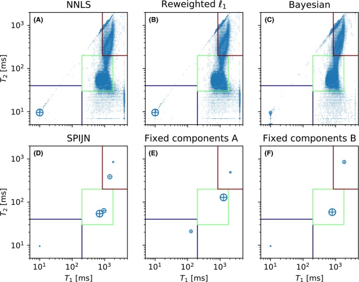
The distribution of the matched components for the 1.5 T in vivo measurement from the 4 different algorithms and an approach with 2 different subdictionaries. The blue box is the short component (myelin water), the green box the middle component (white and gray matter) and the red box the long component (CSF). The size of the circles corresponds to the relative abundance of the components. The subdictionaries contain pre‐fixed components, set A is based on,28 set B on results from the SPIJN algorithm
Figure 5.
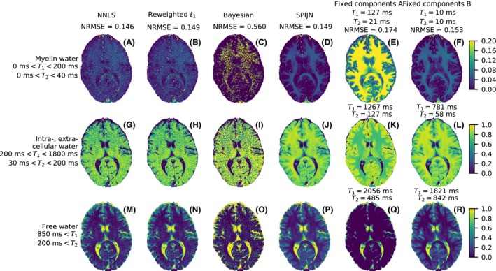
The results of different MC‐MRF algorithms for a brain MRF measurement at 1.5 T. The rows correspond to the different grouped components and the columns to the different algorithms. The last 2 columns contain the results using dictionaries using only 3 components. The color indicates the relative weight of the (grouped) component in each voxel. The first row has a different color scale than the lower 2 rows
The results of the NNLS and the reweighted‐‐norm regularized algorithm are very similar just as for the simulations, but visibly differ from the results of the Bayesian approach. The SPIJN algorithm shows similar structures for the IEW and FW components, but the estimated weights are less noisy compared to the voxel‐wise methods. Although the NRMSE of the NNLS, reweighted‐‐norm regularized and SPIJN algorithm are similar, the introduction of the joint sparsity constraint results in less noise and more clear anatomical structures in the estimated weights.
The results of the 2 MC‐MRF decompositions with 3 fixed components are very different, depending on the chosen combination of relaxation times. Just as the SPIJN algorithm, they show less noise in the estimated weights compared to the voxel‐wise methods. The results of the first set are consistent with the results from,28 but the higher NRMSE indicates a lower consistency with the measured data. The second set of fixed components was based on the results from the SPIJN algorithm and the resulting weights are very similar to the results from the SPIJN algorithm.
The SPIJN algorithm resulted in 5 components, which are shown in Figure 6. These components were grouped to 3 components in Figure 5, which was necessary in order to compare the results of SPIJN to the voxel‐wise algorithms.
Figure 6.
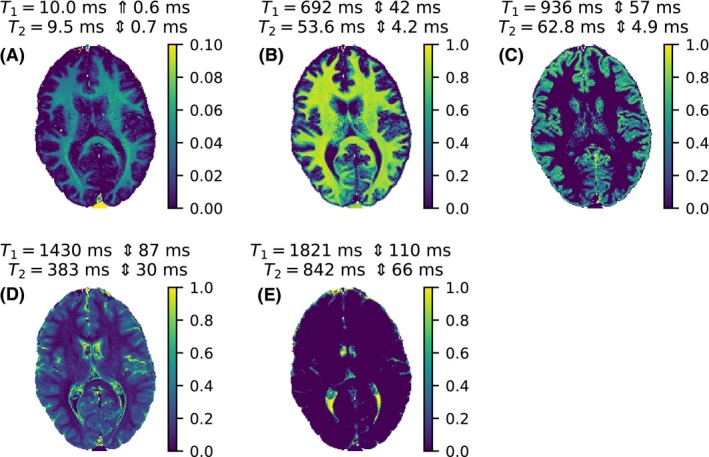
The 5 components matched by the SPIJN algorithm for a measurement at 1.5 T. The color indicates the relative weight of the component in each voxel. The relaxation times for the different components are given. To indicate the grid spacing at a certain point the symbol ⇕ is used, indicating the average distance to the next lower and next higher relaxation time for the matched combination. The relaxation times of component a are related to myelin water, the relaxation times of component b to white mater, the relaxation times of component c to gray matter and the relaxation times of components d and e to CSF
3.2. Repeatability of the SPIJN multi‐component analysis
The 10 3 T measurements are used to test the repeatability over multiple healthy volunteers. The estimated and relaxation times for the components related to white and gray matter are listed in Table 2. The results for the different measurements are similar and in general within 1 or 2 steps of the dictionary resolution away from the mean value. Except for the relaxation time of the gray matter, the matched values are consistent with literature values25 as tabulated in Table 1. While a single component is reconstructed for white matter with our decomposition, the voxels corresponding to gray matter also had a contribution from a component with longer relaxation times.
Table 2.
The matched relaxation times for the white matter and gray matter component for measurements at 10 volunteers at 3T
| White matter (mean 898.1 ms) | Gray matter (mean 1241.0 ms) | ||||||||||
|---|---|---|---|---|---|---|---|---|---|---|---|
| Relaxation time (ms) | 829.26 | 881.00 | 935.96 | 994.35 | 1056.39 | 1192.32 | 1266.70 | 1345.73 | |||
| Grid step size (ms) | 50.22 | 53.35 | 56.68 | 60.21 | 63.97 | 72.20 | 76.71 | 81.49 | |||
| Count | 1 | 6 | 2 | 1 | 2 | 1 | 4 | 3 | |||
|
White matter
|
Gray matter
|
||||||||||
| Relaxation time (ms) | 49.58 | 53.64 | 58.03 | 49.58 | 53.64 | 58.03 | 62.78 | 67.92 | |||
| Grid step size (ms) | 3.90 | 4.22 | 4.57 | 3.90 | 4.22 | 4.57 | 4.94 | 5.35 | |||
| Count | 4 | 4 | 2 | 1 | 1 | 5 | 2 | 1 | |||
Only 4 components were matched by the SPIJN algorithm in the 3 T brain measurements. These estimated component weights are shown for 1 volunteer in Figure 7. Component a and b are assumed to be related to white and gray matter respectively, whereas the other 2 components can be attributed to CSF.
Figure 7.

The 4 components matched by the SPIJN algorithm for a measurement at 3.0 T. The color indicates the relative weight of the component in each voxel. The relaxation times for the different components are given. To indicate the grid spacing at a certain point the symbol ⇕ is used, indicating the average distance to the next lower and next higher relaxation time for the matched combination. The relaxation times of component a are related to white mater, the relaxation times of component b to gray matter and the relaxation times of components c and d to CSF
4. DISCUSSION
A new algorithm with joint sparsity constraint was proposed to perform a MC‐MRF analysis. The SPIJN algorithm was theoretically described and its basic feasibility was demonstrated in simulations and in vivo brain measurements. The proposed algorithm was compared to other recently proposed algorithms for MC‐MRF analysis as well as to the NNLS algorithm, and the repeatability of the results was demonstrated in 10 healthy volunteers.
A first, general observation from the performed experiments is that the NNLS and the reweighted‐‐norm regularized algorithm give very similar results. Both algorithms try to solve the same mathematical problem, but the NNLS algorithm is much faster without the need for regularization. Second, the results from the Bayesian approach were significantly different compared to the other algorithms. This can be explained by the absence of the non‐negativity constraint during the iterations of the algorithm.
To compare the voxel‐wise algorithms to the SPIJN algorithm, the results were grouped based on ranges. Using larger grouping regions enables including all matched components, generally leading to smoother fraction maps, but the grouped relaxation times are less related. When using smaller regions, it is more likely to miss components, leading to noisier tissue fraction maps. Thus, the visualization of voxel‐wise methods is a difficult problem and the provided visualization may not be optimal for each of the individual algorithms, but nevertheless provides some basis of comparison between the results of different algorithms.
The numerical simulations showed that the proposed SPIJN algorithm can separate 3 components with improved accuracy and precision compared to voxel‐by‐voxel MC‐MRF approaches, with a FOV of 100 voxels and 10 voxels per component weight combination. This indicates that the joint sparsity constraint can improve the stability of the ill‐posed inverse problem of MC‐MRF already with a small number of voxels. Therefore, a patch‐based approach, in which the joint sparsity is applied on small local neighborhoods is feasible, and could be an alternative to the global joint sparsity investigated in this work.
The results from the in vivo data in Figure 5 show that the SPIJN algorithm finds a small number of components that form a common basis for the measured MRF signal of the entire ROI, without significantly increasing the representation error compared to voxel‐by‐voxel MC‐MRF approaches. The relaxation times of these components are centered within clusters formed by the relaxation times obtained by the voxel‐by‐voxel algorithms on the (‐) plane. The SPIJN algorithm results in a similar noise level in the component weights as the approach with 3 fixed, a priori chosen components, but it additionally has the freedom to better adapt the chosen components to the data. The components obtained by the SPIJN algorithm can be interpreted as basis tissues that compose the tissue within each voxel and form the mixed signal measured in MRF. These components are recovered merely with the assumption of sparsity and don't necessarily need to correspond to known physical tissues. Depending on the coherence of the dictionary and the selected regularization parameters, it is possible that multiple components would be recovered as a single mixed component or a single component is split into multiple in the decomposition. While the ability of the algorithm to accurately separate multiple components was confirmed in simulations, in‐vivo validation is more difficult since the number of components is unknown.
Nevertheless, in the performed experiments, the resulting MC‐MRF decompositions showed similarities to decompositions presented in previous works9, 10, 11 and can be related to known anatomical structures. With the proposed algorithm, 5 components were observed for the 1.5 T measurement: one component that could be related to a MW component, 2 components related to white matter and gray matter that were grouped to IEW for the comparison, and 2 more components can be interpreted as free water. The weight of the MW component of 5% is lower than the MWF as known from relaxation measurements (typically 10%). Although the results were much noisier, all algorithms were able to recover the MW component in the simulations, and the NNLS and reweighted‐‐norm regularized algorithm also resulted in a MW component of about 5% in the in vivo data. For the 3 T measurements, using a different MRF sequence, 4 components were recovered. These are similar to the last 4 components found in the 1.5 T experiment and can be related to white matter, gray matter and CSF, for which 2 components were found. Similar to,7, 10 no short component that can be attributed to MW was recovered for these data.
These results suggest that the number of components and the corresponding weights depend on the MRF sequence. Different sequences may have different sensitivity to short components. Differences in the estimated MWF were also reported between DESPOT and MESE measurements, supporting the dependence on the acquisition method. By showing these different results for the 2 similar sequences we want to stress the influence of the sequence on the recovered components and the relevance f this as a topic of future research.
In addition, data inconsistencies due to an incomplete model used for the computation of the dictionary may bias the estimation of the component weights. compensation was included for the 3 T data, however, further effects like diffusion or magnetization transfer that were not considered may introduce potential bias. It would be interesting to investigate how more parameters can be efficiently included in the multi‐component analysis and their effect on the component estimation.
The proposed algorithm gives consistent results over repeated measurement in 10 volunteers as shown in Table 2. Direct comparison with literature values is difficult, since these studies do not take in to account the multi‐component effects. Furthermore the literature values from different studies are not very consistent (see Table 1), probably because of differences in the parameter mapping sequences and fitting procedures, different segmentation tools, and potentially certain natural variation between volunteers. However, even a rough comparison can be useful in order to better understand the results from the multi‐component analysis. Performing such a comparison, we see that most relaxation times are in the range of ffkiliterature values, only the of gray matter (mean 58.8 ms) is slightly shorter than the shortest value (65 ms) reported in literature, which was from an Gradient‐spoiled MRF measurement,26 but within the uncertainty range. Most parts of the gray matter are not matched as 1 component, but as a combination of component b and d (see Figure 7), where the latter has long relaxation times, which will lead to longer relaxation times for single component matching.
As already reported in,8, 10 MC‐MRF is more sensitive to noise and the signal perturbations from undersampling can cause significant noise amplification in the estimated weights. One can use very long sequences with few thousand time points in order to gain back the SNR lost by undersampling. In this work, we chose to use a relatively short fully sampled MRF sequence instead, in order to ensure practical processing times for the computationally demanding approaches7, 8 used in the comparisons. It is known that advanced reconstruction methods30, 31, 32, 33 can be applied to reconstruct artifact free image series from the undersampled MRF data, which enables the application of multi‐component analysis on undersampled data with short MRF sequences (see Supporting Information Figure S1). The optimal choice of the MRF sequence and the reconstruction method are out of the scope of this study, but will be interesting topics for future research.
In this study, the regularization parameter was selected such that it minimizes the number of components without increasing the NRMSE compared to regularized voxel‐wise methods, which was used as quality measure of the fit. Alternatively, the regularization parameter can be chosen in a way that specific number of components are recovered, or estimated with methods similar to the misfit used for T2NNLS.3
A requirement from the non‐negativity constraint is that the signal and dictionary are real valued. For the FISP MRF sequence with constant TE it is possible to make this required transformation from a complex to a real signal, since the phase is constant for all time points. When a different MRF acquisition is used, resulting in temporal phase evolution, the phase difference between dictionary and signal may be more challenging to determine. When this phase is determined, the real and imaginary part of the signal can be concatenated to a real signal to perform the MC‐MRF analysis.
This initial technical feasibility study was performed on healthy volunteers only. The ability to capture different tissues or pathology depends on the sensitivity of the used MRF sequence for the tissue of interest. Based on the results from Badve et al34 we think brain tumors would result in 1 or 2 extra components. Investigating the proposed algorithm, the effects of the regularization parameter and influence of the MRF sequence for MC‐MRF in patients would be an important step toward the validation of the approach.
5. CONCLUSION
The sparsity promoting iterative joint NNLS (SPIJN) algorithm was proposed to solve the multi‐component MRF problem through the introduction of a joint sparsity constraint. The introduction of the joint sparsity constraint leads to a higher robustness to noise compared to existing methods and results in a small number of components matched throughout the ROI. This makes the results directly interpretable without further assumptions or complex regrouping strategies. The proposed algorithm finds a small number of components in MRF brain measurements,that can be attributed to known anatomical structures and requires a minimum of further processing of the results. The proposed algorithm is over 10 times faster than previously proposed algorithms for multi‐component MR fingerprinting analysis, which facilitates the potential application of the method in a clinical setting.
Supporting information
FIGURE S1 Results from partial volume estimation based on k‐means clustering as proposed by Deshmane et al6 applied to the 1.5T MC‐MRF measurement as used for Figure 6. MRF‐mapped relaxation times from a single component matching are used for a k‐means clustering method to determine the k = 3 main tissue components. The NNLS algorithm is used to find a multi‐component solution with the subdictionary containing these 3 components. The k‐means clustering method, with a fixed number of components, results in pure tissues in most of the voxels, in contrast to the SPIJN algorithm
FIGURE S2 The effect of undersampling on the MC‐MRF decomposition using the SPIJN algorithm. Fully sampled data from an MRF acquisition using Sequence 1 was retrospectively undersampled with an undersampling factor of 12. This dataset was iteratively reconstructed with matrix‐completion.32 Figure S1A shows the results of the SPIJN algorithm for fully sampled data, Figure S1B shows the results for the iteratively reconstructed undersampled data. The matched components are at most one grid step apart and the resulting fraction maps are almost identical
Nagtegaal M, Koken P, Amthor T, et al. Fast multi‐component analysis using a joint sparsity constraint for MR fingerprinting. Magn Reson Med. 2020;83:521–534. 10.1002/mrm.27947
REFERENCES
- 1. Ma D, Gulani V, Seiberlich N, et al. Magnetic resonance fingerprinting. Nature. 2013;495:187–192. [DOI] [PMC free article] [PubMed] [Google Scholar]
- 2. Tohka J. Partial volume effect modeling for segmentation and tissue classification of brain magnetic resonance images: a review. World J Radiol. 2014;6:855–864. [DOI] [PMC free article] [PubMed] [Google Scholar]
- 3. Whittall KP, MacKay AL. Quantitative interpretation of NMR relaxation data. J Magn Reson (1969). 1989;84:134–152. [Google Scholar]
- 4. Lawson CL, Hanson RJ. Solving Least Squares Problems. SIAM. 1995;15:337. [Google Scholar]
- 5. Whittall KP, Mackay AL, Graeb DA, Nugent RA, Li DKP, Paty DW. In vivo measurement of T2 distributions and water contents in normal human brain. Magn Reson Med. 1997;37:34–43. [DOI] [PubMed] [Google Scholar]
- 6. Deshmane A, McGivney DF, Ma D, et al. Partial volume mapping using magnetic resonance fingerprinting. NMR Biomed. 2019;32:e4082. [DOI] [PubMed] [Google Scholar]
- 7. McGivney D, Deshmane A, Jiang Y, et al. Bayesian estimation of multicomponent relaxation parameters in magnetic resonance fingerprinting: Bayesian MRF. Magn Reson Med. 2018;80:159–170. [DOI] [PMC free article] [PubMed] [Google Scholar]
- 8. Tang S, Fernandez‐Granda C, Lannuzel S, et al. Multicompartment magnetic resonance fingerprinting. Inverse Prob. 2018;34:094005. [DOI] [PMC free article] [PubMed] [Google Scholar]
- 9. McGivney D, Jiang Y, Ma D, Badve C, Gulani V, Griswold M. Segmentation of brain tissues using a Bayesian estimation of multicomponent relaxation values in magnetic resonance fingerprinting. In Proceedings of the 26th Annual Meeting of ISMRM, Paris, France, 2018, p. 1022.
- 10. Duarte R, Repetti A, Gómez PA, Davies M, Wiaux, Y . Greedy approximate projection for magnetic resonance fingerprinting with partial volumes. arXiv:1807.06912 [eess], July 2018.
- 11. Kim D, Wisnowski JL, Nguyen CT, Haldar JP. Relaxation‐relaxation correlation spectroscopic imaging (RR‐CSI): leveraging the blessings of dimensionality to map in vivo microstructure. arXiv:1806.05752 [eess], June 2018. [DOI] [PMC free article] [PubMed]
- 12. Hwang D, Du YP. Improved myelin water quantification using spatially regularized non‐negative least squares algorithm. J Magn Reson Imaging. 2009;30:203–208. [DOI] [PubMed] [Google Scholar]
- 13. Kumar D, Siemonsen S, Heesen C, Fiehler J, Sedlacik J. Noise robust spatially regularized myelin water fraction mapping with the intrinsic B1‐error correction based on the linearized version of the extended phase graph model. J Magn Reson Imaging. 2016;43:800–817. [DOI] [PubMed] [Google Scholar]
- 14. Kumar D, Hariharan H, Faizy TD, et al. Using 3D spatial correlations to improve the noise robustness of multi component analysis of 3D multi echo quantitative T2 relaxometry data. NeuroImage. 2018;178:583–601. [DOI] [PMC free article] [PubMed] [Google Scholar]
- 15. Kim D, Haldar JP. Greedy algorithms for nonnegativity‐constrained simultaneous sparse recovery. Signal Process. 2016;125:274–289. [DOI] [PMC free article] [PubMed] [Google Scholar]
- 16. McGivney DF, Pierre E, Ma D, et al. SVD compression for magnetic resonance fingerprinting in the time domain. IEEE Trans Med Imaging. 2014;33:2311–2322. [DOI] [PMC free article] [PubMed] [Google Scholar]
- 17. Pati YC, Rezaiifar R, Krishnaprasad PS. Orthogonal matching pursuit: Recursive function approximation with applications to wavelet decomposition. In Proceedings of 27th Asilomar Conference on Signals, Systems and Computers, Pacific Grove, CA, USA; vol. 1, November 1993; pp. 40–44. [Google Scholar]
- 18. Foucart S, Koslicki D. Sparse recovery by means of nonnegative least squares. IEEE Signal Process Lett. 2014;21:498–502. [Google Scholar]
- 19. Duarte MF, Sarvotham S, Baron D, Wakin MB, Baraniuk RG. Distributed compressed sensing of jointly sparse signals. In Proceedings of the 2005 Asilomar Conference on Signals, Systems, and Computers, Pacific Grove, CA, USA, IEEE, 2005; p. 1537–1541. ISBN 978‐1‐4244‐0131‐4. [Google Scholar]
- 20. Cotter SF, Rao BD, Engan K, Kreutz‐Delgado K. Sparse solutions to linear inverse problems with multiple measurement vectors. IEEE Trans Signal Process. 2005;53:2477–2488. [Google Scholar]
- 21. Tropp JA, Gilbert AC, Strauss MJ. Algorithms for simultaneous sparse approximation. Part I: greedy pursuit. Signal Process. 2006;86:572–588. [Google Scholar]
- 22. Tropp JA. Algorithms for simultaneous sparse approximation. Part II: convex relaxation. Signal Process. 2006;86:589–602. [Google Scholar]
- 23. Blanchard JD, Cermak M, Hanle D, Jing Y. Greedy algorithms for joint sparse recovery. IEEE Trans Signal Process. 2014;62:1694–1704. [Google Scholar]
- 24. Warntjes M, Engström M, Tisell A, Lundberg P. Modeling the presence of myelin and edema in the brain based on multi‐parametric quantitative MRI. Front Neurol. 2016:7. [DOI] [PMC free article] [PubMed] [Google Scholar]
- 25. Hasgall PA, Di Gennaro F Baumgartner C, et al. It’ is database for thermal and electromagnetic parameters of biological tissues. https://itis.swiss/virtual‐population/tissue‐properties/, Version 4.0, May 15, 2018.
- 26. Jiang Y, Ma D, Seiberlich N, Gulani V, Griswold MA. MR fingerprinting using fast imaging with steady state precession (FISP) with spiral readout. Magn Reson Med. 2015;74:1621–1631. [DOI] [PMC free article] [PubMed] [Google Scholar]
- 27. Hennig J. Multiecho imaging sequences with low refocusing flip angles. J Magn Reson (1969). 1988;78:397–407. [Google Scholar]
- 28. Deshmane A, Badve C, Rogers M, et al. Tissue mapping in brain tumors with partial volume magnetic resonance fingerprinting (PV‐MRF). In Proceedings of the 23rd Annual Meeting of ISMRM, Toronto, Canada, 2015, p. 0071.
- 29. Bojorquez JZ, Bricq S, Acquitter C, Brunotte F, Walker PM, Lalande A. What are normal relaxation times of tissues at 3 T? Magn Reson Imaging. 2017;35:69–80. [DOI] [PubMed] [Google Scholar]
- 30. Davies M, Puy G, Vandergheynst P, Wiaux Y. A compressed sensing framework for magnetic resonance fingerprinting. SIAM J Imaging Sci. 2014;7:2623–2656. [Google Scholar]
- 31. Pierre EY, Ma D, Chen Y, Badve C, Griswold MA. Multiscale reconstruction for MR fingerprinting. Magn Reson Med. 2016;75:2481–2492. [DOI] [PMC free article] [PubMed] [Google Scholar]
- 32. Doneva M, Amthor T, Koken P, Sommer K, Börnert P. Matrix completion‐based reconstruction for undersampled magnetic resonance fingerprinting data. Magn Reson Imaging. 2017;41:41–52. [DOI] [PubMed] [Google Scholar]
- 33. Assländer J, Cloos MA, Knoll F, Sodickson DK, Hennig J, Lattanzi R. Low rank alternating direction method of multipliers reconstruction for MR fingerprinting: low rank ADMM reconstruction. Magn Reson Med. 2018;79:83–96. [DOI] [PMC free article] [PubMed] [Google Scholar]
- 34. Badve C, Yu A, Dastmalchian S, et al. MR fingerprinting of adult brain tumors: initial experience. Am J Neuroradiol. 2017;38:492–499. [DOI] [PMC free article] [PubMed] [Google Scholar]
Associated Data
This section collects any data citations, data availability statements, or supplementary materials included in this article.
Supplementary Materials
FIGURE S1 Results from partial volume estimation based on k‐means clustering as proposed by Deshmane et al6 applied to the 1.5T MC‐MRF measurement as used for Figure 6. MRF‐mapped relaxation times from a single component matching are used for a k‐means clustering method to determine the k = 3 main tissue components. The NNLS algorithm is used to find a multi‐component solution with the subdictionary containing these 3 components. The k‐means clustering method, with a fixed number of components, results in pure tissues in most of the voxels, in contrast to the SPIJN algorithm
FIGURE S2 The effect of undersampling on the MC‐MRF decomposition using the SPIJN algorithm. Fully sampled data from an MRF acquisition using Sequence 1 was retrospectively undersampled with an undersampling factor of 12. This dataset was iteratively reconstructed with matrix‐completion.32 Figure S1A shows the results of the SPIJN algorithm for fully sampled data, Figure S1B shows the results for the iteratively reconstructed undersampled data. The matched components are at most one grid step apart and the resulting fraction maps are almost identical