

Abstract
This paper describes the initial implementation of a new toolbox that seeks to balance accuracy, efficiency, and flexibility in radiation calculations for dynamical models. The toolbox consists of two related code bases: Radiative Transfer for Energetics (RTE), which computes fluxes given a radiative transfer problem defined in terms of optical properties, boundary conditions, and source functions; and RRTM for General circulation model applications—Parallel (RRTMGP), which combines data and algorithms to map a physical description of the gaseous atmosphere into such a radiative transfer problem. The toolbox is an implementation of well‐established ideas, including the use of a k‐distribution to represent the spectral variation of absorption by gases and the use of two‐stream, plane‐parallel methods for solving the radiative transfer equation. The focus is instead on accuracy, by basing the k‐distribution on state‐of‐the‐art spectroscopy and on the sometimes‐conflicting goals of flexibility and efficiency. Flexibility is facilitated by making extensive use of computational objects encompassing code and data, the latter provisioned at runtime and potentially tailored to specific problems. The computational objects provide robust access to a set of high‐efficiency computational kernels that can be adapted to new computational environments. Accuracy is obtained by careful choice of algorithms and through tuning and validation of the k‐distribution against benchmark calculations. Flexibility with respect to the host model implies user responsibility for maps between clouds and aerosols and the radiative transfer problem, although comprehensive examples are provided for clouds.
Keywords: radiation, atmospheric model, parameterization
Key Points
RTE+RRTMGP is a new freely available toolbox for radiation calculations for dynamical models
RTE+RRTMGP seeks to balance accuracy, efficiency, and flexibility, defined expansively
Both code and data continue to evolve to explore different balances among these goals
1. Why Build Another Radiation Parameterization
The ultimate energy source for all atmospheric motions is electromagnetic radiation emitted by the Sun and by the planet and its atmosphere. The flow of radiative energy through the atmosphere depends strongly on the state of the surface and the atmosphere itself. Essentially any model of the atmospheric motions, therefore, has to represent the flow of radiation through the atmosphere. In particular, the vertical gradients of radiative fluxes within the atmosphere and especially at the surface are critical to atmospheric simulation because radiative flux convergence is a major source of atmospheric heating and cooling. Models aimed at understanding climate must also accurately compute the net energy at the top of the atmosphere.
The representation of radiation is one of the most pure exercises in parameterization in atmospheric models because the solution to fully specified problems is known to great accuracy. (This can be contrasted with convection parameterizations, for which sensitive dependence on initial conditions makes fully deterministic prediction essentially impossible, or cloud microphysics, for which some governing equations are not known.) Accuracy across a wide range of clear‐sky conditions can be measured by comparison to benchmark models (Oreopoulos et al., 2012; Pincus et al., 2015), which are themselves known to be in excellent agreement with observations (Alvarado et al., 2013; Mlawer et al., 2000; Turner et al., 2004). Benchmark models also exist for clouds, though observational validation is far more challenging.
The ideas underlying state‐of‐the‐art radiative transfer parameterizations have been established for decades. Radiation is assumed not to propagate in the horizontal (the Independent Column Approximation), reducing the dimensionality of the radiative transfer problem. The complex spectral structure of absorption by gases is treated by grouping optically similar spectral regions using either a correlated k‐distribution (e.g., Fu & Liou, 1992; Lacis & Oinas, 1991) or, less commonly, by modeling transmission using an exponential sum fit of transmissivities (Wiscombe & Evans, 1977). The optical properties of condensed materials, such as clouds and aerosols, are computed in advance, usually as functions of one or more bulk parameters such as effective radius, and fit to tables or functional forms. The resulting problem is solved using versions of the radiative transfer equation in which the angular dependence has been reduced analytically. Though innovations continue, for example in efforts to treat the impact of three‐dimensional transport on radiation fields (Hogan et al., 2016; Schäfer et al., 2016), major conceptual advances in the parameterization of radiation are infrequent.
The maturity of ideas, the near‐universal need for radiation parameterizations, and the substantial effort involved in building an end‐to‐end parameterization mean that radiation codes tend to be developed as complete packages and that these packages, and especially the interfaces to them, have long lifetimes. The codes used by the U.K. Met Office have their roots in the work of Edwards and Slingo (1996). In the United States, many atmospheric models, including both regional and global models developed at the National Center for Atmospheric Research and the National Weather Service's Global Forecast System, use the parameterization RRTM for General circulation model applications (RRTMG; Mlawer et al., 1997). These packages are comprehensive, using information about the physical state of the atmosphere to provide values of spectrally integrated radiative flux.
But conceptual maturity and the black‐box nature of radiation codes can hide important errors. The accuracy of radiation parameterizations can be judged by comparison to reference line‐by‐line models with high angular resolution; every such comparison over the last two‐and‐a‐half decades (e.g., Collins, 2001; Ellingson et al., 1991; Oreopoulos et al., 2012; Pincus et al., 2015) has identified significant parameterization errors in the treatment of gaseous absorption and scattering. These errors partly reflect different efforts to balance computational cost and accuracy, but they also arise because groups may be slow to incorporate new spectroscopic knowledge. Updates to the widely used HITRAN database (Rothman et al., 2013, 2009) over the last decades, for example, have tended to increase the amount of solar radiation absorbed by water vapor. Underestimating this absorption has important consequences for calculations of hydrologic sensitivity (DeAngelis et al., 2015; Fildier & Collins, 2015). The likelihood of errors increases when parameterizations are used to make calculations far outside the range of conditions on which they are trained, for example in calculations on exoplanets (e.g., Yang et al., 2016). Even the highly elevated concentrations of CO2 frequently used to estimate climate sensitivity (Gregory, 2004) represent a challenge for some parameterizations (Pincus et al., 2015).
Complete packages developed for one application may not be easy to adapt to unforeseen uses. Every existing radiation package of which we are aware assumes a particular orientation in the vertical dimension, requiring the reordering of data when the convention in the radiation package differs from that of the host model. Many require separate clear‐ and all‐sky calculations at each invocation where only the latter are needed to advance the host model. None that we are aware of provide the ability to specify an upper boundary condition. As a result, models with shallow domains have to specify an atmospheric profile for use in the radiation scheme alone, complicating implementation and requiring unnecessary computation. In practice, too, most packages tightly couple two conceptually different problems: the mapping of atmospheric state to optical properties and the subsequent calculation of fluxes (i.e., determining the radiative transfer problem and determining the solution to a given problem).
Finally, while every process parameterization seeks to minimize computational cost, efficiency is an acute concern for radiation packages because each calculation is so time‐consuming. The cost is so great that, in many applications, radiation is computed less frequently than other processes by factors of 10–20 (see, e.g., section 2.1 in Hogan & Bozzo, 2018). Computational efficiency is not a static target, however, because computing platforms and approaches (e.g., Balaji et al., 2016) changes rapidly even if the underlying algorithms do not. Even today, an implementation that is efficient on traditional processors is likely to be poorly structured for specialized but highly efficient hardware such as general‐purpose Graphical Processing Units (GPUs).
This paper describes the initial implementation of a new toolbox that seeks to balance accuracy, efficiency, and flexibility in radiation calculations for dynamical models. The toolbox consists of two related code bases: Radiative Transfer for Energetics (RTE), which computes fluxes given a fully specified radiative transfer problem, and RRTMG—Parallel (RRTMGP), which maps a physical description of the aerosol‐ and cloud‐free atmosphere into a radiative transfer problem. Although every line of RTE+RRTMGP is new, the code descends from RRTMG (Clough et al., 2005; Iacono et al., 2000; Mlawer et al., 1997), a parameterization with similar capabilities developed roughly 20 years ago. It also incorporates many of the lessons learned in the development of PSrad (Pincus & Stevens, 2009, 2013), a reimplementation of RRTMG built to explore an idea that required extensive refactoring of the original code. Like its predecessors, RRTMGP uses a k‐distribution for computing the optical properties and source functions of the gaseous atmosphere based on profiles of temperature, pressure, and gas concentrations, while RTE computes fluxes using the Independent Column Approximation in plane‐parallel geometry.
Below, we describe how the design of RTE+RRTMGP balances the sometimes‐conflicting goals of accuracy, efficiency, and flexibility; explain how the k‐distributions are constructed; and assess the accuracy of the current model against more detailed calculations.
2. An Extensible Architecture for Flexibility
The calculation of radiative fluxes for dynamical models presents a particular computational challenge among parameterizations. To treat the enormous spectral variability of absorption by the many optically active gases in the atmosphere, a relatively small amount of state information, that is, profiles of temperature, pressure, and gas concentrations, must be mapped into optical properties (the parameters need to solve the radiative transfer equation) at a number of spectral quadrature points. The optical properties of other constituents such as clouds and aerosols are computed at the same spectral points and added to the values of the gaseous atmosphere. Fluxes are computed independently at each spectral quadrature point. Users, however, normally require only integrals over the spectrum (or portions of it), so spectrally resolved fluxes are summed, greatly reducing the amount of data used by the host model.
As a result of this structure, the radiation problem has an exceptional opportunity to exploit fine‐grained parallelism. Much of the problem is atomic, meaning that calculations are independent in space and the spectral dimension. Transport calculations, while not purely atomic, are independent in the spectral and horizontal dimensions (the latter as a result of the Independent Column Approximation), while spectral reduction is independent in both the horizontal and vertical dimensions. Exploiting this parallelism is key to computational efficiency although the optimal ordering varies across different stages of the computation. RTE and RRTMGP operate on multiple columns at a time to exploit this parallelism. The column dimension is innermost; despite good reasons for having the spectral dimension vary fastest (Hogan & Bozzo, 2018), this choice allows user control over vector length and can be easily adapted to different architectures.
RTE and RRTMGP are agnostic to the ordering of the vertical axis.
2.1. Designing for Robustness
Like the recently developed ecRad package (Hogan & Bozzo, 2018), RTE+RRTMGP cleanly separates conceptually distinct aspects of the radiation problem from one another. Each component, including the gas optics and source function calculations, any implementations of aerosol and cloud optics and methods for computing radiative transfer (transport) can be modified or replaced independently. RTE+RRTMGP is implemented in Fortran 2003. Many components are implemented as Fortran classes that package together code and data. As described below, many of the classes are user extensible to permit greater flexibility. The radiative transfer solvers are straightforward functions.
The Fortran 2003 classes simplify control and information passing, as described below, but basic computational tasks are isolated as kernels, simple procedures with language‐neutral interfaces. The computational kernels are implemented in Fortran 90 with C‐language bindings including the explicit runtime specification of array sizes. Kernels expect sanitized input and do no error checking, so they can be compact and efficient. Separating computational kernels from flow control is also intended to enhance flexibility: It would be possible to build front ends in other languages including Python or C++, using the Fortran class structure or any alternative that suited the problem at hand and still exploit the efficient Fortran kernels. It would also be possible to replace the default kernels with other implementations. We have explored this possibility in prototype kernels optimized for GPUs using OpenACC directives.
The class structure is also aimed at minimizing the amount of data passed to and from the radiation calculation, reducing latency, and increasing efficiency when radiation is implemented on dedicated computational resources (e.g., Balaji et al., 2016) and especially on devices such as GPUs.
Other conventions aim to make RTE+RRTMGP more portable across platforms and environments. The precision of all REAL variables is explicitly set via a Fortran KIND parameter so that a one character change in a single file can produce single‐ or double‐precision versions of the code. RTE+RRTMGP uses few thresholds, but most are expressed relative to working precision. Most procedures are implemented as functions returning character strings; empty strings indicate success, while non‐empty strings contain error messages. RTE+RRTMGP does not read or write to files. Instead, classes that require data such as lookup tables at initialization use load functions with flat array arguments so that users can read and distribute data consistent with their local software environment.
2.2. Specifying and Solving the Radiative Transfer Equation: RTE
The components of RTE+RRTMGP communicate through sets of spectrally dependent optical properties. Optical properties are described by their spectral discretization: the number of bands and the spectral limits of each band in units of wavenumber (inverse centimeters). Each band covers a continuous region of the spectrum, but bands need not be disjoint or contiguous. Anticipating the spectral structure provided by gas optics parameterizations like RRTMGP, each band may be further subdivided into g‐points. Each spectral point is treated as a independent pseudo‐monochromatic calculation.
Optical properties may be specified as sets of numerical values on a column/height/spectral grid. Each of the three possible set of values is represented as a discrete subclass of the general optical properties class. The “scalar” class includes only the absorption optical depth τ a, as is required for computing radiative transfer in the absence of scattering; the “two‐stream” class includes extinction optical depth τ e, single‐scattering albedo ω 0, and asymmetry parameter g; while the “n‐stream” class contains τ e, ω 0, and phase function moments p, as required by four‐stream or other discrete ordinates calculations. (The dependence on two spatial coordinates and a spectral coordinate is left implicit.)
Using a class structure allows user interaction to be greatly simplified. As one example, sets of optical properties on the same grid can be added together in a single call, with the class structure invoking the correct kernel depending on which two sets of optical properties are provided. Single calls allow optical properties to be delta scaled (Joseph et al., 1976; Potter, 1970) or checked for erroneous values.
Solvers compute radiative fluxes given values of optical properties and appropriate boundary conditions and source function values. A shortwave solver requires specifying the (pseudo‐)spectrally dependent collimated beam at the top of the model, albedos for direct and diffuse radiation at the surface, and the values of optical properties within the atmosphere. A longwave solver requires the optical properties, spectrally dependent surface emissivity, and the values of the Planck source functions at the surface and at each layer and level of the atmosphere.
Calculations that account for scattering, the usual standard for shortwave radiation and a more accurate option for longwave calculations that include clouds (Costa & Shine, 2006; Kuo et al., 2017), use the two‐stream formulation of Meador and Weaver (1980) to compute layer transmittance and reflectance and the adding formulation of Shonk and Hogan (2008) to compute transport (i.e., the fluxes that result from interactions among layers). Two‐stream coupling coefficients in the shortwave come from the “practical improved flux method” formulations of Zdunkowski et al. (1980); the longwave follows Fu et al. (1997). The accuracy of longwave calculations that neglect scattering may be increased through the use of first‐order Gaussian quadrature using up to three terms using weights and directions from Clough et al. (1992). Longwave calculations assume that the source function varies linearly with optical depth. At this writing, RTE does not yet include four‐stream or higher‐order methods for radiative transport.
The set of optical properties provided determines the solution method: When the solvers are called with the subclass representing {τ,ω 0,g}, the two‐stream/adding solver is invoked; if only τ is provided, a calculation neglecting scattering is performed. Solutions are computed for each g‐point in the set of optical properties independently, allowing RTE to solve problems for any spectral structure.
All solvers allow for the specification of incoming diffuse radiation at the top of the domain (this flux is otherwise assumed to be 0). We originally imagined that this capability would be most useful in the simulation of very shallow domain by fine‐scale models (e.g., Seifert et al., 2015). Experience implementing RTE+RRTMGP in global models, however, suggests that it may also be a useful alternative to the common practice of adding an extra layer above the model top in radiation calculations.
Because radiative fluxes are computed from optical properties, there is no explicit treatment of clouds and particularly of internal cloud variability or its structure in the vertical. Subgrid variability may be accounted for by random sampling in the spectral dimension using the Monte Carlo Independent Column Approximation (Pincus et al., 2003). Extensions to the plane‐parallel equations that rely on an explicit clear/cloudy partitioning, including the TripleClouds algorithm for treating partial cloudiness (Shonk & Hogan, 2008) or the SPARTACUS extension for treating the subgrid‐scale effects of three‐dimensional radiative transport (Hogan et al., 2016; Schäfer et al., 2016), are not consistent with this framework.
The RTE solvers compute fluxes for each spectral point independently, but the full spatial and spectral detail is unlikely to be useful in most contexts. It is, on the other hand, hard to know precisely what users might need. One approach would be to implement an expansive set of output variables, perhaps allowing user control over which are computed, but this can be cumbersome and requires changes to the radiation code to add a new output.
RTE takes a conceptually more complicated but practically simpler approach: Output from RTE solvers is provided through a user‐extensible Fortran 2003 class. The class must include storage for the desired results and code to compute those results from the full profiles of fluxes at each spectral point. In particular, the class must implement a reduction function (so named because it reduces the amount of output) with arguments specified by RTE. These arguments include the spectral discretization information and the vertical ordering, enabling the computation of very specific quantities (during design we had in mind the calculation of photosynthetically active radiation at the surface). Examples are provided that compute broadband fluxes (spectrally integrated up, down, net, and direct if available) and fluxes within each band. Users provide this class in the call to the solver; the solvers, in turn, call the reduction function after spectrally dependent fluxes are calculated, minimizing the amount of information returned from RTE.
2.3. Computing the Optical Properties of the Gaseous Atmosphere: RRTMGP
RTE provides methods for solving a spectrally detailed radiative transfer problem; its complement, RRTMGP, determines the parameters of such a radiative transfer problem for the gaseous component of the atmosphere given the physical state and composition. RRTMGP encapsulates the calculation of gas optics, that is, the calculation of τ a or {τ e,ω 0,g} and the associated source functions, given pressure, temperature, and gas concentrations within the domain. RRTMGP builds on RTE: The classes representing gas optics and the Planck functions extend the generic representation of optical properties, and the gas optics calculation returns a set of optical property values.
RRTMGP includes a general framework for representing gas optics. One piece of this framework is a class describing the concentrations of gases within the atmosphere. The volume mixing ratio of each gas is provided as a name‐value pair, where the name is normally the chemical formula (e.g., “ch4” or “h2o”). Values may be provided as scalars, if the gas is well‐mixed, as profiles assumed constant in the horizontal, or varying in the horizontal and vertical dimensions.
The second piece of the general framework, an abstract gas optics class, defines a minimal set of interfaces for functions that map atmospheric state to optical properties. Codes written to use this generic interface can seamlessly use any concrete instance of the abstract class. This approach is motivated by the desire to explore hierarchies of detail in the treatment of absorption by gases (Tan et al., 2019; Vallis et al., 2018) without requiring substantial recoding.
RRTMGP gas optics is a concrete instance of the abstract gas optics class that uses a k‐distribution to represent the spectral variation of absorption coefficients. Data and code are entirely distinct in RRTMGP's gas optics: The class is initialized with data provided in a netCDF file (though RRTMGP does not read the file directly, for reasons explained above). The ability to provide data at runtime, available for more than 20 years in the radiation codes used by the U.K. Met Office (Edwards & Slingo, 1996), provides flexibility, including the provisioning of data with accuracy matched to application needs, as well as a way to incorporate new spectroscopic knowledge as it become available, so that models can stay up‐to‐date without code changes. The class representing gas concentrations must also be supplied when initializing RRTMGP gas optics so that the tables of absorption coefficients may be thinned to include only those gases for which concentrations are provided, reducing impacts on memory and computation time.
2.4. Mapping Concepts to Software
Figure 1 illustrates the class structure by which RTE+RRTMGP is organized. The figure highlights the capabilities described in sections 2.2 and 2.3. Not shown are initialization and finalization procedures, procedures for extracting subsets from values defined with a column dimension (available for source functions, optical properties, and gas concentrations), or the procedures by which the spectral discretization can be set and queried.
Figure 1.
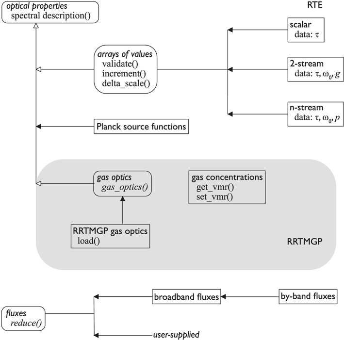
Class organization for RTE+RRTMGP. Class names are in sans serif fonts and data and procedures in serif. Arrows indicate inheritance: Classes inherit the data and procedures and/or interfaces provided by their parents. Ovals, open arrowheads, and italicized class names represent abstract classes providing functionality and/or specifying procedures to be provided by descendent classes. Calculations require concrete classes (unitalicized names, rectangles). Solvers are implemented as procedures using these classes as inputs or to compute outputs. The figure illustrates only the most important functionality within each class; most implement more procedures than are shown. RTE = Radiative Transfer for Energetics; RTTMGP = RRTM for General circulation model applications—Parallel.
Figure 1 emphasizes the distinction between optics, which map atmospheric conditions defined on a spatial grid onto spectrally dependent values of optical properties and source functions, and stored sets of these values defined on a spatial and spectral grid. RRTMGP is a map for the gaseous component of the atmosphere. As we note above, users must provide analogous maps for condensed species. In most applications, users will initialize these maps (e.g., RRTMGP gas optics, user‐provided aerosol, and cloud optics) with data at the beginning of a simulation. Each calculation of radiative fluxes made during the course of a simulation uses those maps to determine the optical properties of each component of the atmosphere, defines a set of problems to be solved (e.g., clear‐sky as the sum of gases and aerosols and all‐sky as the sum of clear‐sky and clouds), and invokes the solvers on each problem, summarizing results to meet (problem‐specific) user requirements.
3. Accuracy and Efficiency
3.1. Developing a New Treatment of Absorption by Gases
RRTMGP treats absorption by gases using a k‐distribution (Ambartsumian, 1936; Fu & Liou, 1992; Goody et al., 1989; Lacis & Oinas, 1991) in which an integral over frequency ν is replaced by an integral over the variable g defined such that absorption coefficient k(g) increases monotonically (and hence much more smoothly). This integral is further approximated by a discrete sum over G quadrature points using an average absorption coefficient at each point. The mapping is normally computed for a set of bands within which absorption is dominated by one or two gases though alternatives are possible (Hogan, 2010). The map varies with the state of the atmosphere, so there is no inherent relationship between g‐points and wavelengths. For RRTMGP, the bands are disjoint, contiguous, and essentially span the set of frequencies of radiation emitted by the Sun or Earth.
As is described in more detail below, the k‐distribution is first generated for a range of atmospheric conditions following an automated procedure and then tuned by adjusting these absorption coefficients and the related source functions by hand so that fluxes and their sensitivity to composition perturbations, computed over a set of training profiles, are in agreement with line‐by‐line reference calculations. Appendix A contains greater detail about the k‐distribution and how it is discretized.
3.1.1. Automated Generation of a k‐Distribution
The version of RRTMGP data described here is based on high‐accuracy calculations with the Line‐By‐Line Radiative Transfer Model (LBLRTM; Clough et al., 2005), which has undergone extensive cycles of evaluation with observations and subsequent improvement (see, e.g., Alvarado et al., 2013; Mlawer et al., 2012) and agrees with well‐calibrated spectrally resolved radiometric measurements. Results below are based on LBLRTM_v12.8, line parameter file aer_v_3.6 (itself based, to a large extent, on the HITRAN 2012 line file described by Rothman et al., 2013), and continuum model MT_CKD_3.2. All are available online (https://rtweb.aer.com). Shortwave calculations are based on the solar source function of Lean and DeLand (2012).
In the automated step, computations of optical depth are made with LBLRTM for a set of pressure and temperature values, spanning the range of present‐day conditions to define the spectral map. Reference volume mixing ratios for water vapor and ozone are based on a large number of profiles from the Modern‐Era Retrospective Analysis for Research and Applications, version 2 reanalysis (MERRA2, see Randles et al., 2017) and vary with temperature, with distinct reference values for pressures greater than or less than 10,000 Pa. Other species use a constant reference value.
RRTMGP follows RRTMG in defining bands so that absorption within each band is dominated by no more than two gases termed that band's “major species.” Some bands have no major species. Dry air is used as the second major species in bands in which absorption is dominated by a single gas, which increases accuracy modestly while simplifying implementation. Computations are made for range of relative abundances 0 ≤ η ≤ 1 of the two major species where and denotes volume mixing ratio χ i normalized by its reference value , with concentrations of all other gases held fixed at their respective reference values. The total optical depth, including contributions from major and all minor species, determines the spectral map .
Given this spectral map, the absorption coefficients for the major species are derived from LBLRTM calculations of absorption optical depth τ a(p,T,η) in single atmospheric layers containing only the major species in question. Optical depth values are mapped from frequency ν to g, averaged across a predetermined number G of g intervals, and converted to absorption coefficients k(g) by dividing by the combined column amount , where W i is defined as the layer‐integrated molecular amount (molecules per cm2) of major species i.
For longwave bands, the same mapping is used to calculate the “Planck fraction,” defined as the fraction of the band‐integrated Planck energy (uniquely determined by T) associated with each g‐point within the band. The solar source function for each g‐point is constant at present; Appendix A describes how these values are obtained.
The contributions of other absorbing species are handled with less detail than are major species. A single representative pressure p 0(T) is chosen for each “minor species.” LBLRTM is used to calculate the spectrally dependent absorption coefficient of this species in isolation as a function of temperature. The coefficients are ordered using and averaged within each of the G intervals. Rayleigh scattering optical depths follow the same approach.
Absorption by both major and minor species is treated separately in the upper and lower atmosphere (pressures above and below 10,000 Pa). Distinct sets of gases are used in each domain. Some gases are considered below 100 hPa but not above, or vice versa, depending on the degree to which they influence fluxes.
The discretization of the k‐distribution available at this writing, including details about the spectral discretization (“bands”), the gases considered within each band, and the density of the tabulated data, are provided in Appendix A. Given this tabulated information, RRTMGP computes absorption coefficients and Planck fractions for arbitrary atmospheric conditions by linearly interpolating the tabulated values in , and η. Optical depths are computed by multiplying the interpolated absorption coefficient by the combined column amount of the layer in question. Interpolation algorithms are as general as possible so that, for example, the same code is used for contributions that depend only on absorber abundance and those that also depend on the abundance of other gases, such as collision‐induced absorption and foreign continua. Planck source functions are determined by multiplying the Planck fractions by band‐integrated Planck source functions tabulated on a fine temperature grid.
3.1.2. Testing and Tuning the Correlated k‐Distribution
We evaluate the accuracy of the initial k‐distribution by computing fluxes for a set of 42 clear‐sky atmospheric profiles (Garand et al., 2001) that span a large range of temperature, moisture, and ozone abundances and include baseline concentrations of other gases. Results from RTE+RRTMGP for these training atmospheres are compared to LBLRTM calculations. We minimize differences due to transport algorithms by using the same set of three quadrature angles in LBLRTM and RTE for longwave problems; in the shortwave, we focus on the direct beam since this depends only on the optical depth. For shortwave assessments, the solar zenith angle is 30°; for longwave calculations, the surface emissivity is 1.
Fluxes computed across the set of atmospheres using the initial k‐distribution are in substantially better agreement with reference calculations than are fluxes computed with RRMTG (Figure 2), primarily because RRTMGP is based on the same underlying spectroscopy as the benchmark.
Figure 2.

Accuracy of RRTMGP's new k‐distribution, assessed as the difference between fluxes computed with RTE+RRTMGP and those from the reference calculations across the set of training atmospheres. LW calculations compare high spectral resolution line‐by‐line and parameterized calculations using identical transport algorithms, while the SW comparison focused only on the direct solar beam at the surface and so requires no multiple‐scattering calculations. RRTMGP = RRTMG for General circulation model applications—Parallel; LW= longwave; SW = shortwave; TOA = top of atmosphere.
We also assess the accuracy of RRTMGP in computing instantaneous radiative forcing, that is, the change in flux for these 42 profiles due to increases, relative to nominal preindustrial concentrations, of factors of 2 and 4 for CO2 and CH4 and the change between present‐day and preindustrial concentrations of N2O and halocarbons. The primary focus is on 4×CO2 and 2×CH4.
Accuracy assessments for both flux and forcing guide a hand tuning of the absorption coefficients and source functions. This tuning is holistic, considering a wide range of radiative quantities but focusing primarily on broadband flux and heating rate profiles and the forcing due to individual gases, especially CO2 and CH4. Attention is also paid to flux and heating rate profiles within each band to minimize compensating errors.
In calculations with RTE, the optical properties and source functions provided by RRTMGP gas optics at each g‐point are treated as a set of pseudo‐monochromatic calculations. This is equivalent to assuming that the spectral mapping (or “correlation” between ν and g) is constant through the atmosphere and is what distinguishes a correlated k‐distributions used in vertically inhomogeneous atmosphere from a k‐distribution developed for a single layer. The assumption is an important source of error in correlated k‐distributions. In many circumstances, the true spectral map varies in the vertical, such that the absorption coefficients for a g‐value correspond to different sets of frequencies at different altitudes. As one example, in shortwave bands in which ozone and water vapor both absorb significantly, absorption in the stratosphere is dominated by ozone with a very different spectral structure than the absorption by water vapor in the troposphere, yet absorption due to these two gases will map to the same g‐values at different altitudes. In such circumstances, the lack of consistency with height of the spectral map (a lack of correlation) degrades model accuracy relative to spectrally resolved calculations.
The hand tuning attempts to correct for errors introduced by the assumption of correlation and any other errors (e.g., the relatively simple treatment of minor species). Major species absorption coefficients are adjusted as functions of p and η; minor species coefficients are tuned as functions of T. Adjustments made to Planck fractions are a function of p, while the solar source terms have no dependence on any variables. All source function tunings conserve energy. The ad hoc and empirical tuning is similar in sprit to, but substantially less formal than, the work reported by Sekiguchi and Nakajima (2008), who used an explicit cost function to determine the spectral discretization and integration rules for their k‐distribution.
Tuning modestly improves the accuracy of the k‐distribution (compare the orange and green boxes in Figure 2), decreasing both the bulk of errors and the most extreme errors in our training atmospheres. Forcing is also improved (see the examples in Figure 3). In interpreting these results, recall that the profiles used here are chosen to explore specific sources of error rather than being strictly representative of the distribution of conditions in the Earth's atmosphere.
Figure 3.
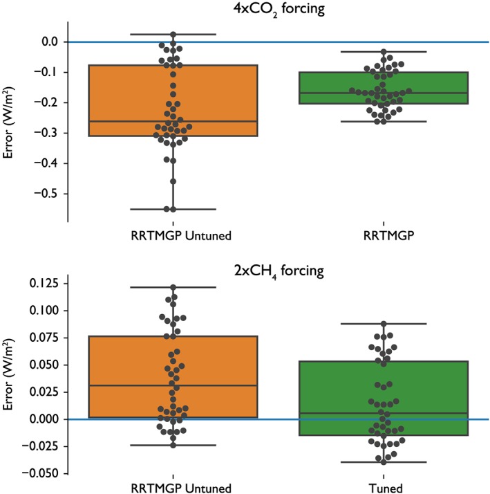
Accuracy of RRTMGP's new k‐distribution for forcing calculations. Shown here are the two primary forcings considered during tuning: impacts on top‐of‐atmosphere longwave fluxes from concentrations of carbon dioxide quadrupled from pre‐industrial concentrations and doubled methane concentrations. As with fluxes, tuning reduces the largest errors and modestly improves the median error across the training data set. RRTMGP = rapid and accurate radiative transfer model for general circulation model applications—Parallel.
3.2. Accuracy: Validation and Verification
Before comparing results from RTE+RRTMGP against reference calculations, we verified RTE against ecRad (Hogan & Bozzo, 2018) by computing broadband fluxes for the training atmospheres with both codes using RRTMGP's representation of gas optics. Differences in fluxes are within 10−8 W/m2 for direct and diffuse shortwave fluxes, reflecting the fact that both packages make the same choices even though they are entirely independent implementations. Differences in longwave fluxes are as large as 10−2 W/m2 due to different formulations of the source function.
The accuracy of fluxes at the atmosphere's boundaries computed by RTE+RRTMGP in its most commonly used configuration is shown in Figure 4; RRTMG is shown for comparison. Here longwave fluxes are computed with a single angle and total fluxes (diffuse plus direct for the shortwave) computed for the training atmospheres are compared against reference line‐by‐line calculations using three angles. Calculations with RRTMG use a diffusivity angle that depends on column‐integrated water vapor in some bands to mimic the three‐angle calculation (e.g., Figure 2). The lack of this correction in RRTMGP increases the error in downwelling longwave flux at the surface, relative to the three‐angle calculations shown in Figure 2, in some atmospheres. (We are currently developing a similar treatment of diffusivity angle for RRTMGP.) Changes in other fluxes are dominated by revisions to spectroscopy so that RRTMGP is substantially more accurate than RRTMG.
Figure 4.
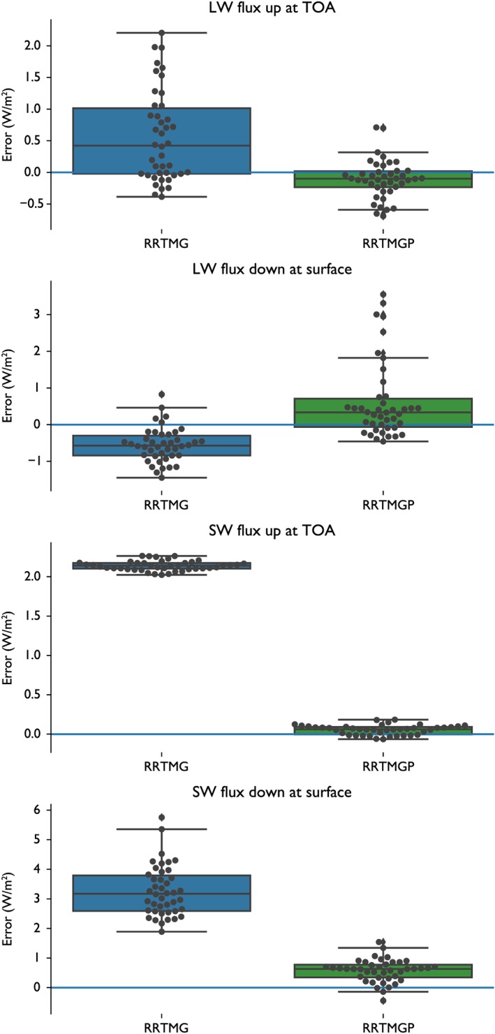
Accuracy of RTE+RRTMGP in producing fluxes at the surface and TOA as judged against line‐by‐line calculations on the set of training atmospheres. RTE uses a single angle calculation (cf. the three‐angle calculation in Figure 2) for the LW calculations in the two upper panels, consistent with normal use. RTE uses a constant diffusivity angle; the increased accuracy from RRTMG's parameterization for this angle as a function of integrated water path is small compared to the differences introduced by updated spectroscopy. SW results show comparisons of total (direct plus diffuse) flux. RTE = Radiative Transfer for Energetics; RRTMGP = RRTMG for General circulation model applications—Parallel; LW = longwave; SW = shortwave; TOA = top of atmosphere.
Figure 5 shows the maximum magnitude of heating rate errors. Pressures greater and less than 10,000 Pa are shown separately because radiative heating rates are much larger in the latter than the former.
Figure 5.
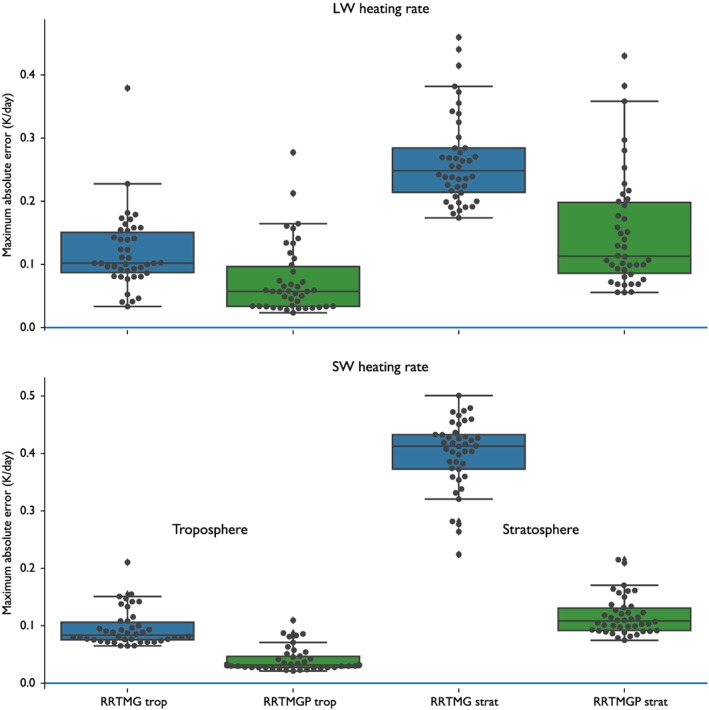
Accuracy of RTE+RRTMGP in producing heating rates. Errors are computed separately for the LW (top panel) and SW (bottom panel) and for the troposphere (left columns) and stratosphere (right columns). Consistent with Figure 4, changes relative to the older spectroscopy of RRTMG are most evident in SW calculations. RRTMGP = RRTM for General circulation model applications—Parallel; LW = longwave; SW = shortwave.
We assess the out‐of‐sample accuracy of RTE+RRTMGP using 100 profiles chosen by the Radiative Forcing Model Intercomparison Project (RFMIP) protocol (Pincus et al., 2016). The profiles were drawn from reanalysis so that the weighted sum of fluxes in the profiles reproduces the change in global‐mean, annual‐mean top‐of‐atmosphere present‐day to preindustrial forcing (the change in flux between atmospheres with present‐day and preindustrial concentrations of greenhouse gases). Relative to high angular‐resolution line‐by‐line calculations with LBLRTM, fluxes computed by RTE+RRTMGP are accurate to within 0.4% at the top of the atmosphere and 0.2% at the surface; absorption by the atmosphere is accurate to about 0.4% for the longwave and 0.8% for the shortwave (see Table 1). Preindustrial to present‐day changes at the atmospheres boundaries are accurate to roughly 5% for longwave change and 12% for the (substantially smaller) shortwave change.
Table 1.
Error (and Reference Value) of Annual‐Mean, Global‐Mean Instantaneous Radiative Forcing (W/m2), for Present‐Day Relative to Preindustrial Conditions, Computed Using 100 Profiles Following the Protocol of the Radiative Forcing Model Intercomparison Project
| Present‐day fluxes | Preindustrial to present‐day change | |||
|---|---|---|---|---|
| Level | Longwave | Shortwave | Longwave | Shortwave |
| Top of atmosphere (up) | 0.033 (263.197) | 0.165 (47.315) | 0.148 (−2.845) | 0.007 (−0.058) |
| Net absorption | −0.749 (−180.696) | −0.610 (72.344) | −0.055 ( 0.803) | −0.051 (0.522) |
| Surface (down) | 0.725 (315.346) | 0.026 (245.553) | −0.095 (2.083) | 0.065 (−0.534) |
Note. Error is computed relative to reference calculations with high angular and spectral resolution. The columns are chosen to characterize the error in forcing; as one consequence average values for fluxes in the present‐day (the first set of columns) is affected by sampling error.
3.3. Efficiency
As one measure of efficiency, we compare the time taken to compute clear‐sky flux profiles for the 1,800 atmospheric conditions (100 profiles for each of 18 perturbations to atmospheric conditions) used in the RFMIP assessment of accuracy. On a dedicated compute node at the National Energy Research Scientific Computing Center, using current Intel compilers and Haswell nodes processing eight columns at a time, RRTMGP is slower than RRTMG by roughly a factor of 2.2 in longwave calculations. RRTMG uses substantially fewer spectral points (140 in the longwave) than does RRTMGP (256); even accounting for this difference, RRTMGP remains about 20% slower than its predecessor. The inefficiency is mostly due to the calculations of gas optics and Planck sources. It arises partly because RRTMGP takes a general approach to the calculation of gas optical depths, where RRTMG's compute paths (e.g., which gases contributed to absorption in each band) were coded by hand and so were more easily optimized. We are working to refactor a few closely related routines to further increase the computational efficiency.
In the shortwave, on the other hand, RRTMGP is about as twice as fast as RRTMG, or almost 4 times faster per g‐point, owing primarily to easily vectorized codes. We have noted substantial variation in these ratios across computing platforms, operating systems, and compilers and caution that real‐life applications may be less efficient than these idealized tests.
4. Tools and Packages
This paper stresses the principles guiding the development and use of RTE+RRTMGP. This is partly because we expect the underlying software to evolve and partly because the principles—designing parameterizations for flexibility and efficiency from the ground up—may be useful in designing other parameterizations. We have stressed our intent to make RTE+RRTMG as flexible as possible with respect to both the computing environment and the context in which radiative calculations are to be made.
One consequence of agnosticism with respect to the host model is that users have substantially more responsibility. This is most obvious in the treatment of clouds and aerosol. The RTE+RRTMGP repository includes examples to compute cloud optics (the map from physical state to optical properties), using a class analogous to the RRTMGP gas optics, and to treat cloud overlap with the Monte Carlo Independent Column Approximation (Pincus et al., 2003), using procedures relying on user‐generated random numbers. The examples are narrow by design and are directly useful only if the assumptions about macrophysics and microphysics are consistent with the host models. The intent of the examples is to be useful as a starting point from which users may build implementations more self‐consistent with the host model's other formulations. The programs used to compute accuracy for RFMIP in section 3.2, also included in the RTE+RRTMGP repository, show how the RRTMGP gas optics is initialized from data and used to compute the inputs needed for RTE, and how output is extracted from RTE, and play a similar role.
Many of the concerns that spurred the development of RTE+RRTMGP have motivated other development efforts. One example is the ecRad code (Hogan & Bozzo, 2018), which was developed contemporaneously. Compared to RTE+RRTMGP, ecRad is more complete (it includes treatments for cloud and aerosol optics and carefully crafted methods for subgrid scale sampling of homogenous clouds) and more capable (it includes alternatives for treating cloud overlap and a parameterization for three‐dimensional transport within each column). The ecRad package represents a complete solution suitable for users who want to make precisely the same choices or are willing to adapt the internals of the package to their own needs. RTE+RRTMGP, in contrast, is intended as an extensible tool or platform on which user‐specific applications can be built by extension rather than modification.
Optics computations—the mapping from model state to a radiative transfer problem—are a form of coupling in which detailed information about both representations is required. From this perspective, the role of RTE is to provide a reasonably flexible representation of the radiative transfer problem and a matched set of methods for solution. The coupling of clouds and aerosols to these problems is left to users because the variety of possible macrophysical and microphysical descriptions is enormous, while the tools required to make the map, such as codes for computing single‐scattering properties using Mie‐Lorenz theory, are widely accessible. Computing the optical properties of the gaseous atmosphere, on the other hand, requires a small and easily enumerable set of inputs but relies on tools and expertise that is less broadly distributed among the community. These considerations explain our choice to link RTE+RRTMGP in both the software sense and in this description.
This paper reports on the initial implementation of RTE+RRTMGP. In particular, the assessments of accuracy in section 3 use a k‐distribution with 16 g‐points per band, for a total of 256 in the longwave and 224 in the shortwave. Experience developing the predecessor RRTMG from its parent model suggests that much of the accuracy of the underlying k‐distribution can be obtained with substantially fewer spectral points (see also Sekiguchi & Nakajima, 2008), making possible substantial increases in efficiency for modest decreases in accuracy. We also anticipate that accuracy in clearly defined applications such as weather forecasting may be able to achieve the same accuracy with less computational cost by reducing the number of spectral points that provide accuracy in instantaneous radiative forcing. We are currently working to provide several sets of absorption coefficients striking different balances between accuracy and efficiency.
Acknowledgments
Code, data, and user documentation for RTE+RRTMGP are available online (https://github.com/RobertPincus/rte-rrtmgp); this manuscript was produced with data and code archived at doi:10.5281/zenodo.3403173. Scripts and data in this paper are available at https://github.com/RobertPincus/rte-rrtmgp-paper-figures (doi:10.5281/zenodo.3362619). The LBLRTM model and associated data used in the accuracy calculations in section 3 are available online (http://rtweb.aer.com). We appreciate design suggestions from Robin J. Hogan of ECMWF and Brian Eaton of NCAR. Benjamin Hillman of Sandia National Lab has identified a number of bugs in prototype implementations. Andre Wehe helped with design and implementation in the early stages of the project. K. Franklin Evans and Rick Pernak provided infrastructure for regression testing, verification, and validation. We are grateful for comments from three anonymous reviewers, which helped sharpen our writing. This work utilized the Janus and RMACC Summit supercomputers, both of which were supported by the National Science Foundation (Janus under Award CNS‐0821794, Summit under awards ACI‐1532235 and ACI‐1532236) and the University of Colorado Boulder. Janus supercomputer was a joint effort of the University of Colorado Boulder, the University of Colorado Denver, and the National Center for Atmospheric Research; Summit a joint effort of the University of Colorado Boulder and Colorado State University. The development of RTE+RRTMPG has been supported to date by the Office of Naval Research under Grants N00014‐13‐1‐0858 and N00014‐17‐1‐2158, by NASA under Grant NNH13CJ92C, and by the Department of Energy's Office of Biological and Environmental Sciences under Grants DE‐SC0012399 and DE‐SC0016593.
Appendix A. RRTMGP's k‐Distribution in Detail
A.1.
Tables A1 and A2 show the band structure adopted in the present version of RRTMGP. The band values in the longwave differ modestly from those in RRTMG. The ordering of shortwave bands is strictly monotonic, abandoning the idiosyncratic ordering of RRTMG. Both changes imply that any fits, for example, for cloud optical properties made for RRTMG will need to be revisited before use in RRTMGP.
Table A1.
Current Rapid and Accurate Radiative Transfer Model for General Circulation Model Applications—Parallel Spectral Structure for the Longwave
| Wavenumber limits | Absorbers (p ≥ 10,000 Pa) | Absorbers (p<10,000 Pa) | |||
|---|---|---|---|---|---|
| Band | (cm−1) | Major | Minor | Major | Minor |
| 1 | 10–250 | H2O | N2 | H2O | N2 |
| 2 | 250–500 | H2O | H2O | ||
| 3 | 500–630 | H2O, CO2 | N2O | H2O, CO2 | N2O |
| 4 | 630–700 | H2O, CO2 | O3, CO2 | ||
| 5 | 700–820 | H2O, CO2 | O3, CCL4, CFC‐22 | O3, CO2 | CCL4, CFC‐22 |
| 6 | 820–980 | H2O | CO2, CFC‐11, CFC‐12, HFC‐143a | — | CFC‐11, CFC‐12, HFC‐143a |
| 7 | 980–1,080 | H2O, O3 | CO2 | O3 | CO2 |
| 8 | 1,080–1,180 | H2O | CO2, O3, N2O, CFC‐12, | O3 | CO2, CO, CFC‐12, |
| CFC‐22, HFC‐23 | CFC‐22, HFC‐23, | ||||
| HFC‐32, HFC‐125, | HFC‐32, HFC‐125, | ||||
| HFC‐134a | HFC‐134a | ||||
| 9 | 1,180–1,390 | H2O, CH4 | N2O, CF4, HFC‐134a, HFC‐143a | CH4 | N2O, CF4,HFC‐134a, HFC‐143a |
| 10 | 1,390–1,480 | H2O | H2O | ||
| 11 | 1,480–1,800 | H2O | O2 | H2O | O2 |
| 12 | 1,800–2,080 | H2O, CO2 | — | ||
| 13 | 2,080–2,250 | H2O, N2O | CO2, CO | — | O3 |
| 14 | 2,250–2,390 | CO2 | CO2 | ||
| 15 | 2,390–2,680 | H2O, CO2 | N2O, N2 | — | |
| 16 | 2,680–3,250 | H2O, CH4 | CH4 | ||
Note. The distinction between major and minor absorbers is explained in section 3.1. Water vapor foreign and self‐continua are also included as minor gases for any bands in which water vapor is a major species.
Table A2.
Current Rapid and Accurate Radiative Transfer Model for General Circulation Model Applications—Parallel Spectral Structure for the Shortwave
| Wavenumber limits | Absorbers (p ≥ 10,000 Pa) | Absorbers (p<10,000 Pa) | |||
|---|---|---|---|---|---|
| Band | (cm−1) | Major | Minor | Major | Minor |
| 1 | 820–2,680 | H2O, CO2 | CH4, N2O, N2 | H2O, CO2 | CH4, N2O, O3 |
| 2 | 2,680–3,250 | H2O, CH4 | CH4 | ||
| 3 | 3,250–4,000 | H2O, CO2 | H2O, CO2 | ||
| 4 | 4,000–4,650 | H2O, CH4 | CH4 | ||
| 5 | 4,650–5,150 | H2O, CO2 | CO2 | ||
| 6 | 5,150–6,150 | H2O | CH4 | H2O | CH4 |
| 7 | 6,150–7,700 | H2O | CO2 | H2O, CO2 | |
| 8 | 7,700–8,050 | H2O, O2 | H2O, O2 | ||
| 9 | 8,050–12,850 | H2O | O2 | H2O | O3 |
| 10 | 12,850–16,000 | H2O, O2 | O3 | H2O, O2 | O3 |
| 11 | 16,000–22,650 | H2O | O3, O2, NO2 | O3 | O2, NO2 |
| 12 | 22,650–29,000 | — | NO2 | — | NO2 |
| 13 | 29,000–38,000 | O3 | O3 | ||
| 14 | 38,000–50,000 | O3, O2 | O3, O2 | ||
Note. The distinction between major and minor absorbers is explained in section 3.1. Water vapor foreign and self‐continua are also included as minor gases for any bands in which water vapor is a major species.
The spectral map is computed at pressures 1 ≤ p ≤ 109,600 Pa in increments of = 0.2, temperatures 160 ≤ T ≤ 355 K in 15‐K increments, and η = 0, 1/8, … 1. When computing η, the mixing ratio of the second major gas v 2 is set to the reference value , and v 1 varies except at η=1, where v 2=0 and .
Band‐integrated values of the Planck function are computed in 1‐K increments.
The g‐point dependence of the solar source function S is determined from the reference line‐by‐line calculations for the 42 atmospheres used for validation (section 3.1.2). For each profile i within this set and within each band b, we identify the pressure at which the direct solar beam has been depleted by 10% and compute the map at the corresponding values of T and η. Although the Garand et al. (2001) atmospheres span a wide range of temperatures and gas abundances, we find relatively little variation among the maps . We therefore compute the average map across the set of profiles and apply this map to the incident solar radiation to determine S(g) for all profiles.
Pincus, R. , Mlawer, E. J. , & Delamere, J. S. (2019). Balancing accuracy, efficiency, and flexibility in radiation calculations for dynamical models. Journal of Advances in Modeling Earth Systems, 11,3074–3089 10.1029/2019MS001621
References
- Alvarado, M. J. , Payne, V. H. , Mlawer, E. J. , Uymin, G. , Shephard, M. W. , Cady‐Pereira, K. E. , Delamere, J. S. , & Moncet, J. L. (2013). Performance of the Line‐By‐Line Radiative Transfer Model (LBLRTM) for temperature, water vapor, and trace gas retrievals: Recent updates evaluated with IASI case studies. Atmospheric Chemistry and Physics, 13(14), 6687–6711. [Google Scholar]
- Ambartsumian, V. (1936). The effect of absorption lines on the radiative equilibrium of the outer layers of stars. Publication of the Astronomical Observatory of Leningrad, 6, 7–18. [Google Scholar]
- Balaji, V. , Benson, R. , Wyman, B. , & Held, I. (2016). Coarse‐grained component concurrency in Earth system modeling: Parallelizing atmospheric radiative transfer in the GFDL AM3 model using the Flexible Modeling System coupling framework. Geoscientific Model Development, 9(10), 3605–3616. [Google Scholar]
- Clough, S. A. , Iacono, M. J. , & Moncet, J.‐L. (1992). Line‐by‐line calculations of atmospheric fluxes and cooling rates: Application to water vapor. Journal of Geophysical Research, 97(D14), 15,761–15,785. [Google Scholar]
- Clough, S. A. , Shephard, M. W. , Mlawer, E. J. , Delamere, J. S. , Iacono, M. J. , Cady‐Pereira, K. , Boukabara, S. , & Brown, P. D. (2005). Atmospheric radiative transfer modeling: A summary of the AER codes. Journal of Quantitative Spectroscopy and Radiation Transfer, 91(2), 233–244. [Google Scholar]
- Collins, W. D. (2001). Parameterization of generalized cloud overlap for radiative calculations in general circulation models. Journal of the Atmospheric Sciences, 58(21), 3224–3242. [Google Scholar]
- Costa, S. M. S. , & Shine, K. P. (2006). An estimate of the global impact of multiple scattering by clouds on outgoing long‐wave radiation. Quarterly Journal of the Royal Meteorological Society, 132(616), 885–895. [Google Scholar]
- DeAngelis, A. M. , Qu, X. , Zelinka, M. D. , & Hall, A. (2015). An observational radiative constraint on hydrologic cycle intensification. Nature, 528(7581), 249–253. [DOI] [PubMed] [Google Scholar]
- Edwards, J. M. , & Slingo, A. (1996). Studies with a flexible new radiation code. I: Choosing a configuration for a large‐scale model. Quarterly Journal of the Royal Meteorological Society, 122(531), 689–719. [Google Scholar]
- Ellingson, R. G. , Ellis, J. , & Fels, S. (1991). The intercomparison of radiation codes used in climate models: Long wave results. Journal of Geophysical Research, 96(D5), 8929–8953. [Google Scholar]
- Fildier, B. , & Collins, W. D. (2015). Origins of climate model discrepancies in atmospheric shortwave absorption and global precipitation changes. Geophysical Research Letters, 42, 8749–8757. 10.1002/2015gl065931 [DOI] [Google Scholar]
- Fu, Q. , & Liou, K. N. (1992). On the correlated k‐distribution method for radiative transfer in nonhomogeneous atmospheres. Journal of the Atmospheric Sciences, 49(22), 2139–2156. [Google Scholar]
- Fu, Q. , Liou, K. N. , Cribb, M. C. , Charlock, T. P. , & Grossman, A. (1997). Multiple scattering parameterization in thermal infrared radiative transfer. Journal of the Atmospheric Sciences, 54(24), 2799–2812. [Google Scholar]
- Garand, L. , Turner, D. S. , Larocque, M. , Bates, J. , Boukabara, S. , Brunel, P. , Chevallier, F. , Deblonde, G. , Engelen, R. , Hollingshead, M. , Jackson, D. , Jedlovec, G. , Joiner, J. , Kleespies, T. , McKague, D. S. , McMillin, L. , Moncet, J. L. , Pardo, J. R. , Rayer, P. J. , Salathe, E. , Saunders, R. , Scott, N. A. , Van Delst, P. , & Woolf, H. (2001). Radiance and Jacobian intercomparison of radiative transfer models applied to HIRS and AMSU channels. Journal of Geophysical Research, 106(D20), 24,017–24,031. [Google Scholar]
- Goody, R. , West, R. , Chen, L. , & Crisp, D. (1989). The correlated‐k method for radiation calculations in nonhomogeneous atmospheres. Journal of Quantitative Spectroscopy and Radiation Transfer, 42(6), 539–550. [Google Scholar]
- Gregory, J. M. (2004). A new method for diagnosing radiative forcing and climate sensitivity. Geophysical Research Letters, 31, L03205 10.1029/2003gl018747 [DOI] [Google Scholar]
- Hogan, R. J. (2010). The full‐spectrum correlated‐k method for longwave atmospheric radiative transfer using an effective Planck function. Journal of the Atmospheric Sciences, 67(6), 2086–2100. [Google Scholar]
- Hogan, R. J. , & Bozzo, A. (2018). A flexible and efficient radiation scheme for the ECMWF model. Journal of Advances in Modeling Earth Systems, 10, 1990–2008. 10.1029/2018MS001364 [DOI] [Google Scholar]
- Hogan, R. J. , Schäfer, S. A. K. , Klinger, C. , Chiu, J. C. , & Mayer, B. (2016). Representing 3‐D cloud radiation effects in two‐stream schemes: 2. Matrix formulation and broadband evaluation. Journal of Geophysical Research: Atmospheres, 121, 8583–8599. 10.1002/2016jd024875 [DOI] [Google Scholar]
- Iacono, M. J. , Mlawer, E. J. , Clough, S. A. , & Morcrette, J.‐J. (2000). Impact of an improved longwave radiation model, RRTM, on the energy budget and thermodynamic properties of the NCAR Community Climate Model, CCM3. Journal of Geophysical Research, 105(D11), 14,873–14,890. [Google Scholar]
- Joseph, J. H. , Wiscombe, W. J. , & Weinman, J. A. (1976). The Delta‐Eddington approximation for radiative flux transfer. Journal of the Atmospheric Sciences, 33(12), 2452–2459. [Google Scholar]
- Kuo, C.‐P. , Yang, P. , Huang, X. , Feldman, D. , Flanner, M. , Kuo, C. , & Mlawer, E. J. (2017). Impact of multiple scattering on longwave radiative transfer involving clouds. Journal of Advances in Modeling Earth Systems, 9, 3082–3098. 10.1002/2017ms001117 [DOI] [Google Scholar]
- Lacis, A. A. , & Oinas, V. (1991). A description of the correlated k‐distribution method for modeling non‐grey gaseous absorption, thermal emission, and multiple scattering in vertically inhomogeneous atmospheres. Journal of Geophysical Research, 96(D5), 9027–9063. [Google Scholar]
- Lean, J. L. , & DeLand, M. T. (2012). How does the Sun's spectrum vary? Journal of Climate, 25(7), 2555–2560. [Google Scholar]
- Meador, W. E. , & Weaver, W. R. (1980). Two‐stream approximations to radiative transfer in planetary atmospheres: A unified description of existing methods and a new improvement. Journal of the Atmospheric Sciences, 37(3), 630–643. [Google Scholar]
- Mlawer, E. J. , Brown, P. D. , Clough, S. A. , Harrison, L. C. , Michalsky, J. J. , Kiedron, P. W. , & Shippert, T. (2000). Comparison of spectral direct and diffuse solar irradiance measurements and calculations for cloud‐free conditions. Geophysical Research Letters, 27(17), 2653–2656. 10.1029/2000gl011498 [DOI] [Google Scholar]
- Mlawer, E. J. , Payne, V. H. , Moncet, J. L. , Delamere, J. S. , Alvarado, M. J. , & Tobin, D. C. (2012). Development and recent evaluation of the MTCKD model of continuum absorption. Philosophical Transactions of the Royal Society A, 370(1968), 2520–2556. [DOI] [PubMed] [Google Scholar]
- Mlawer, E. J. , Taubman, S. J. , Brown, P. D. , Iacono, M. J. , & Clough, S. A. (1997). Radiative transfer for inhomogeneous atmospheres: RRTM, a validated correlated‐k model for the longwave. Journal of Geophysical Research, 102(D14), 16,663–16,682. [Google Scholar]
- Oreopoulos, L. , Mlawer, E. , Delamere, J. , Shippert, T. , Cole, J. , Fomin, B. , Iacono, M. , Jin, Z. , Li, J. , Manners, J. , Räisänen, P. , Rose, F. , Zhang, Y. , Wilson, M. J. , & Rossow, W. B. (2012). The continual intercomparison of radiation codes: Results from phase I. Journal of Geophysical Research, 117, D06118 10.1063/1.3117076 [DOI] [Google Scholar]
- Pincus, R. , Barker, H. W. , & Morcrette, J.‐J. (2003). A fast, flexible, approximate technique for computing radiative transfer in inhomogeneous cloud fields. Journal of Geophysical Research, 108(D13), 4376 10.1029/2002jd003322 [DOI] [Google Scholar]
- Pincus, R. , Forster, P. M. , & Stevens, B. (2016). The Radiative Forcing Model Intercomparison Project (RFMIP): Experimental protocol for CMIP6. Geoscientific Model Development, 9, 3447–3460. [Google Scholar]
- Pincus, R. , Mlawer, E. J. , Oreopoulos, L. , Ackerman, A. S. , Baek, S. , Brath, M. , Buehler, S. A. , Cady‐Pereira, K. E. , Cole, J. N. S. , Dufresne, J.‐L. , Kelley, M. , Li, J. , Manners, J. , Paynter, D. J. , Roehrig, R. , Sekiguchi, M. , & Schwarzkopf, D. M. (2015). Radiative flux and forcing parameterization error in aerosol‐free clear skies. Geophysical Research Letters, 42, 5485–5492. 10.1002/2015gl064291 [DOI] [PMC free article] [PubMed] [Google Scholar]
- Pincus, R. , & Stevens, B. (2009). Monte Carlo spectral integration: A consistent approximation for radiative transfer in large eddy simulations. Journal of Advances in Modeling Earth Systems, 1, 1 10.3894/james.2009.1.1 [DOI] [Google Scholar]
- Pincus, R. , & Stevens, B. (2013). Paths to accuracy for radiation parameterizations in atmospheric models. Journal of Advances in Modeling Earth Systems, 5, 225–233. 10.1002/jame.20027 [DOI] [Google Scholar]
- Potter, J. F. (1970). The delta function approximation in radiative transfer theory. Journal of the Atmospheric Sciences, 27(6), 943–949. [Google Scholar]
- Randles, C. A. , da Silva, A. M. , Buchard, V. , Colarco, P. R. , Darmenov, A. , Govindaraju, R. , Smirnov, A. , Holben, B. , Ferrare, R. , Hair, J. , Shinozuka, Y. , & Flynn, C. J. (2017). The MERRA‐2 Aerosol Reanalysis, 1980 onward. Part I: System description and data assimilation evaluation. Journal of Climate, 30(17), 6823–6850. [DOI] [PMC free article] [PubMed] [Google Scholar]
- Rothman, L. S. , Gordon, I. E. , Babikov, Y. , Barbe, A. , Chris Benner, D. , Bernath, P. F. , Birk, M. , Bizzocchi, L. , Boudon, V. , Brown, L. R. , Campargue, A. , Chance, K. , Cohen, E. A. , Coudert, L. H. , Devi, V. M. , Drouin, B. J. , Fayt, A. , Flaud, J. M. , Gamache, R. R. , Harrison, J. J. , Hartmann, J. M. , Hill, C. , Hodges, J. T. , Jacquemart, D. , Jolly, A. , Lamouroux, J. , Le Roy, R. J. , Li, G. , Long, D. A. , Lyulin, O. M. , Mackie, C. J. , Massie, S. T. , Mikhailenko, S. , M ller, H. S. P. , Naumenko, O. V. , Nikitin, A. V. , Orphal, J. , Perevalov, V. , Perrin, A. , Polovtseva, E. R. , Richard, C. , Smith, M. A. H. , Starikova, E. , Sung, K. , Tashkun, S. , Tennyson, J. , Toon, G. C. , Tyuterev, V. G. , & Wagner, G. (2013). The HITRAN2012 molecular spectroscopic database. Journal of Quantitative Spectroscopy and Radiation Transfer, 130(0), 4–50. [Google Scholar]
- Rothman, L. S. , Gordon, I. E. , Barbe, A. , Benner, D. C. , Bernath, P. F. , Birk, M. , Boudon, V. , Brown, L. R. , Campargue, A. , Champion, J. P. , Chance, K. , Coudert, L. H. , Dana, V. , Devi, V. M. , Fally, S. , Flaud, J. M. , Gamache, R. R. , Goldman, A. , Jacquemart, D. , Kleiner, I. , Lacome, N. , Lafferty, W. J. , Mandin, J. Y. , Massie, S. T. , Mikhailenko, S. N. , Miller, C. E. , Moazzen‐Ahmadi, N. , Naumenko, O. V. , Nikitin, A. V. , Orphal, J. , Perevalov, V. I. , Perrin, A. , Predoi‐Cross, A. , Rinsland, C. P. , Rotger, M. , Simeckova, M. , Smith, M. A. H. , Sung, K. , Tashkun, S. A. , Tennyson, J. , Toth, R. A. , Vandaele, A. C. , & Vander Auwera, J. (2009). The HITRAN 2008 molecular spectroscopic database. Journal of Quantitative Spectroscopy and Radiation Transfer, 110(9–10), 533–572. [Google Scholar]
- Schäfer, S. A. K. , Hogan, R. J. , Klinger, C. , Chiu, J. C. , & Mayer, B. (2016). Representing 3‐D cloud radiation effects in two‐stream schemes: 1. Longwave considerations and effective cloud edge length. Journal of Geophysical Research: Atmospheres, 121, 8567–8582. 10.1002/2016jd024876 [DOI] [Google Scholar]
- Seifert, A. , Heus, T. , Pincus, R. , & Stevens, B. (2015). Large‐eddy simulation of the transient and near‐equilibrium behavior of precipitating shallow convection. Journal of Advances in Modeling Earth Systems, 7, 1918–1937. 10.1002/2015ms000489 [DOI] [Google Scholar]
- Sekiguchi, M. , & Nakajima, T. (2008). A k‐distribution‐based radiation code and its computational optimization for an atmospheric general circulation model. Journal of Quantitative Spectroscopy and Radiation Transfer, 109(17‐18), 2779–2793. [Google Scholar]
- Shonk, J. K. P. , & Hogan, R. J. (2008). Tripleclouds: An efficient method for representing horizontal cloud inhomogeneity in 1D radiation schemes by using three regions at each height. Journal of Climate, 21(11), 2352–2370. [Google Scholar]
- Tan, Z. , Lachmy, O. , & Shaw, T. A. (2019). The sensitivity of the jet stream response to climate change to radiative assumptions. Journal of Advances in Modeling Earth Systems, 11, 934–956. 10.1029/2018ms001492 [DOI] [Google Scholar]
- Turner, D. D. , Tobin, D. C. , Clough, S. A. , Brown, P. D. , Ellingson, R. G. , Mlawer, E. J. , Knuteson, R. O. , Revercomb, H. E. , Shippert, T. R. , Smith, W. L. , & Shephard, M. W. (2004). The QME AERI LBLRTM: A closure experiment for downwelling high spectral resolution infrared radiance. Journal of the Atmospheric Sciences, 61(22), 2657–2675. [Google Scholar]
- Vallis, G. K. , Colyer, G. , Geen, R. , Gerber, E. , Jucker, M. , Maher, P. , Paterson, A. , Pietschnig, M. , Penn, J. , & Thomson, S. I. (2018). Isca, v1.0: A framework for the global modelling of the atmospheres of Earth and other planets at varying levels of complexity. Geoscientific Model Development, 11(3), 843–859. [Google Scholar]
- Wiscombe, W. J. , & Evans, J. W. (1977). Exponential‐sum fitting of radiative transmission functions. Journal of Computational Physics, 24(4), 416–444. [Google Scholar]
- Yang, J. , Leconte, J. , Wolf, E. T. , Goldblatt, C. , Feldl, N. , Merlis, T. , Wang, Y. , Koll, D. D. B. , Ding, F. , Forget, F. , & Abbot, D. S. (2016). Differences in water vapor radiative transfer among 1D models can significantly affect the inner edge of the habitable zone. Astrophysical Journal, 826(2), 222. [Google Scholar]
- Zdunkowski, W. G. , Welch, R. M. , & Korb, G. J. (1980). An investigation of the structure of typical two‐stream methods for the calculation of solar fluxes and heating rates in clouds. Beiträge zur Physik Atmosphëre, 53, 147–166. [Google Scholar]