Propensity‐score matching with competing risks in survival analysis

Abstract

Propensity‐score matching is a popular analytic method to remove the effects of confounding due to measured baseline covariates when using observational data to estimate the effects of treatment. Time‐to‐event outcomes are common in medical research. Competing risks are outcomes whose occurrence precludes the occurrence of the primary time‐to‐event outcome of interest. All non‐fatal outcomes and all cause‐specific mortality outcomes are potentially subject to competing risks. There is a paucity of guidance on the conduct of propensity‐score matching in the presence of competing risks. We describe how both relative and absolute measures of treatment effect can be obtained when using propensity‐score matching with competing risks data. Estimates of the relative effect of treatment can be obtained by using cause‐specific hazard models in the matched sample. Estimates of absolute treatment effects can be obtained by comparing cumulative incidence functions (CIFs) between matched treated and matched control subjects. We conducted a series of Monte Carlo simulations to compare the empirical type I error rate of different statistical methods for testing the equality of CIFs estimated in the matched sample. We also examined the performance of different methods to estimate the marginal subdistribution hazard ratio. We recommend that a marginal subdistribution hazard model that accounts for the within‐pair clustering of outcomes be used to test the equality of CIFs and to estimate subdistribution hazard ratios. We illustrate the described methods by using data on patients discharged from hospital with acute myocardial infarction to estimate the effect of discharge prescribing of statins on cardiovascular death.

1. INTRODUCTION

Investigators are increasingly using observational studies to estimate the effects of treatments, exposures, and interventions. However, a consequence of the lack of random treatment assignment is that treated subjects often differ systematically at baseline from control subjects. Due to the confounding that occurs when the distribution of subject characteristics differ between treated and control subjects, outcomes cannot be compared directly between treated and control subjects. Instead, statistical methods must be used to remove the effects of the observed confounding. Statistical methods based on the propensity score are being used with increasing frequency in observational studies examining the effect of treatments. The propensity score is defined as a subject's probability of receiving the active treatment of interest conditional on measured baseline covariates.1, 2 There are four ways of using the propensity score: matching on the propensity score, inverse probability of treatment weighting (IPTW) using the propensity score, stratification on the propensity score, and covariate adjustment using the propensity score. Of the four methods of using the propensity score, matching on the propensity score is particularly popular in the medical literature.3, 4, 5

Survival or time‐to‐event outcomes occur frequently in biomedical and epidemiological research.6 Several papers have examined the use of propensity score methods with time‐to‐event outcomes.7, 8, 9, 10, 11 The focus of these papers was on the application of propensity score methods in settings with a single cause of failure (eg, all‐cause mortality). Competing risks are events whose occurrence precludes the occurrence of the primary event of interest.12, 13, 14 If the primary event of interest was time to death due to cardiovascular causes, then death due to non‐cardiovascular causes would serve as a competing risk, as subjects who die of non‐cardiovascular causes are no longer at risk of death due to cardiovascular causes. In general, all non‐fatal outcomes and all cause‐specific mortality outcomes are subject to competing risks. Despite the frequency with which competing risks are present in medical and epidemiological research, there is a paucity of research describing how propensity score methods should be used in settings with competing risks.

Historically, conventional regression adjustment has been the most popular method to account for confounding when using observational data to estimate the effects of treatments and interventions. However, there are several limitations to this approach. First, when outcomes are binary or time‐to‐event in nature, regression adjustment limits the investigator to reporting adjusted odds ratios or hazard ratios, which are relative measures of effect. Several different clinical commentators have argued that reporting relative measures of effects provides insufficient information to fully inform clinical decision making.15, 16, 17, 18, 19 Instead, at the very least, relative measures of effect should be complemented by absolute measures of effect (such as risk differences) and measures derived from them, such as the number needed to treat (NNT). When outcomes are time‐to‐event in nature, analyses based on the propensity score can provide the information on both relative and absolute measures of treatment effect that are necessary to inform clinical decision making.9, 10, 20 A second difference between multivariable regression adjustment and propensity score methods is the target estimand. Multivariable regression adjustment has a conditional (or subject‐specific) target estimand, while propensity‐score methods have marginal (or population‐average) target estimand.21 The latter is the estimand that is also the target in randomized controlled trials. Finally, matching on the propensity score permits estimation of the average treatment effect in the treated (ATT). Thus, if the study question centers on the effect of treatment in those who were ultimately treated, matching on the propensity score permits addressing this question. In contrast to this, multivariable regression adjustment does not directly permit estimation of the effect of treatment in those subjects who were treated.

The objective of the current paper is to discuss the application of propensity‐score matching in settings in which competing risks are present. The paper is structured as follows. In Section 2, we describe statistical methods for estimating the effect of treatment in settings with competing risks when using propensity‐score matching. In Section 3, we describe the design of a series of Monte Carlo simulations that were used to compare methods to test equality of cumulative incidence functions (CIFs) between treatment groups in propensity‐score matched samples and to estimate subdistribution hazard ratios. In Section 4, we report the results of the Monte Carlo simulations. In Section 5, we present a brief case study to illustrate the application of these methods when using propensity‐score matching. Finally, in Section 6, we summarize our findings and discuss them in the context of the existing literature.

2. STATISTICAL METHODS FOR PROPENSITY‐SCORE MATCHING IN THE PRESENCE OF COMPETING RISKS

Several studies have examined the application of propensity score methods to settings with time‐to‐event or survival outcomes.7, 9, 10, 11, 20 In this section, we describe how these methods can be modified for use with propensity‐score matching in settings with competing risks.

2.1. Learning from analyses in RCTs

When designing and analyzing a retrospective study, Dorn22 asked the question “How would the study be conducted if it were possible to do it by controlled experimentation?” Rubin suggests that this question is of key importance, as it defines the objective of an observational study.23 These sentiments suggest that the analyses conducted in a study that uses propensity‐score matching should reflect, to the greatest degree possible, the analyses that would be conducted in an RCT with a similar treatment and outcome.

Several sets of authors have suggested that absolute measures of treatment effect are superior to relative measures of treatment effect for making treated‐related decisions for patients.15, 16, 17 Other authors have suggested that, at the very least, the reporting of relative measures of effect should be supplemented by the reporting of absolute measures of effect.18, 19 In its instructions to authors, the BMJ (British Medical Journal) requires that, for any RCT with a dichotomous outcome, absolute risk reductions and the associated number needed to treat (NNT) be reported.24 These commentaries suggest that, in RCTs with survival outcomes, authors report both the absolute and relative effects of treatment. Absolute effects of treatment can be estimated by comparing survival curves between treatment groups. From these, the NNT can be computed at any duration of follow‐up.25 The relative effect of treatment can be determined from a Cox proportional hazards model in which the hazard of the event is regressed on treatment status. The resultant measure of effect is the hazard ratio which quantifies the relative change in the hazard of the event due to treatment.

As we move to consider the corresponding analyses when using propensity‐score matching in the presence of competing risks, we suggest that estimating the relative effect of treatment is comparable to estimating the relative effect of treatment on the cause‐specific hazard function, while estimating the absolute effect of treatment is comparable to estimating the effect of treatment on the CIF. These analyses are described in the following two sub‐sections.

2.2. Estimating the relative effect of treatment on the cause‐specific hazard function when using propensity‐score matching

In the setting with time‐to‐event outcomes and competing risks, the cause‐specific hazard function for the kth event type is a function of time (t) that is defined as ${\lambda }_k^{cs}\left(t\right)=\underset{\mathrm{\Delta }t\to 0}{\lim }\frac{\text{Prob}\left(t\le T<t+\mathrm{\Delta }tD=k|T\ge t\right)}{\mathrm{\Delta }t}$, where T is the time at which an event occurred and D is a variable denoting the type of event that occurred (with D = k denoting that the kth event type has occurred). The cause‐specific hazard function for the kth event type can be interpreted as the instantaneous rate of occurrence of the kth event type in subjects who are currently event‐free (eg, subjects for whom no event of any type has occurred).

The cause‐specific hazard model for the kth event type allows one to estimate the association of covariates with the cause‐specific hazard function for the kth event type: ${\lambda }_k^{cs}\left(t\right)={\lambda }_{0k}^{cs}\left(t\right)\exp \left(\beta \mathbf{X}\right)$, where ${\lambda }_{0k}^{cs}\left(t\right)$ denotes the baseline cause‐specific hazard function for the kth event type, and X denotes a vector of covariates. In practice, the cause‐specific hazard model can be fit using standard statistical software for fitting the Cox proportional hazards model. To do so, one censors subjects who experience a competing event at the time that the competing event occurs (eg, a subject who experiences a competing event at time t_ce is treated as though they were censored at time t_ce and were no longer under observation from that time onwards). The estimated regression coefficients can be interpreted as denoting the association of the covariate with the rate at which the event of interest occurs in subjects who are currently event‐free.

When using propensity‐score matching, the relative effect of treatment on the outcome can be estimated using a cause‐specific hazard model, in which the cause‐specific hazard of the outcome of interest is regressed on an indicator variable denoting treatment status. As matching on the propensity score has balanced the distribution of observed covariates between treatment groups, it is not necessary to adjust for other baseline covariates. When using propensity‐score matching, a robust variance estimator can be used to account for the matched nature of the sample.7 Fitting such a model allows investigators to test whether the rate of the occurrence of the outcome in subjects who are currently event‐free is the same between treated and control subjects in the matched sample.

There are two different ways in which one could account for the matched nature of the sample: one can fit a marginal model that uses a robust variance estimator to account the clustering of subjects in matched pairs. Alternatively, one could fit a cause‐specific model that stratified on the matched pairs, thereby allowing the baseline hazard function to vary across matched sets. Previous research has shown that the former results in unbiased estimation of marginal hazard ratios, whereas the latter results in biased estimation of marginal hazard ratios.7 The reason for the bias when stratifying on the matched pairs is that this model is implicitly a conditional model. For this reason, we recommend that a marginal model with a robust variance estimator be used. This issue will be explored in the Monte Carlo simulations described below for the scenario when one is testing the equality of CIFs estimated in matched treated and control subjects.

2.3. Estimating the effect of treatment on the CIF when using propensity‐score matching

In the absence of competing risks, the incidence of events over time is typically estimated using the complement of the Kaplan‐Meier survival function. However, in the presence of competing risks, the Kaplan–Meier estimate will be biased upwards.12, 13, 14 Thus, using estimates of absolute changes in the incidence of the outcome based on differences in Kaplan–Meier survival functions may be biased.

The cumulative cause‐specific hazard function for the kth event type is defined as ${\mathrm{\Lambda }}_k\left(t\right)={\int }_0^t{\lambda }_k^{cs}\left(s\right)\mathrm{d}s$. The overall survival function is defined as $S\left(t\right)=\text{exp}\left(-{\sum }_{k=1}^K{\mathrm{\Lambda }}_k\left(t\right)\right)$, where S(t) denotes the probability of not failing of any cause by time t: S(t) =  Pr (T ≥ t). The CIF for the kth event type is defined as F_k(t) =  Pr (T ≤ t, D = k). It is the probability of experiencing the kth event type prior to time t. It can be expressed in terms of the cause‐specific hazard function as $F_k\left(t\right)={\int }_0^t{\lambda }_k^{cs}\left(s\right)S\left(s\right)\mathrm{d}s$. Note that as this expression involves the overall survival function, which is a function of all K cause‐specific hazard functions, the CIF implicitly involves knowledge of the K cause‐specific hazard functions, and it is insufficient to have information on only the cause‐specific hazard function for the event of interest.

Instead of using the complement of the Kaplan–Meier function, authors should estimate the CIF in each treatment group separately. This can be done by first estimating the CIF in the matched treated subjects and then by estimating the CIF in the matched control subjects. The difference between the estimated CIF function in the treated and control groups provides an estimate of the absolute reduction in the incidence of the outcome at different times. The reciprocal of the difference in CIF functions provides an estimate of the NNT in the presence of competing risks.26

Fine and Gray introduced the subdistribution hazard function for the kth event type: ${\lambda }_k^{sd}\left(t\right)=\underset{\mathrm{\Delta }t\to 0}{\lim }\frac{\text{Prob}\left(t<T\le t+\mathrm{\Delta }tD=k|T>t\cup \left(T<t\cap K\ne k\right)\right)}{\mathrm{\Delta }t}$.27 It denotes the instantaneous rate of failure from the kth event in subjects who have not yet experienced an event of that type. Note that this risk set includes those who are currently event free as well as those who have previously failed from a competing event. The Fine‐Gray subdistribution hazard model is a model for the CIF: it allows one to estimate the effect of covariates on the CIF. The direction of the subdistribution hazard ratio provides information of the direction of treatment on the cumulative incidence of the outcome. However, similarly to survival data without competing risks, the magnitude of this hazard ratio does not provide direct information on the magnitude of the relative effect of the treatment on the cumulative incidence function.28

Gray's test can be used to test the equality of CIFs between independent samples.29 It is unclear how best to test the equality of CIFs between treated and control subjects in a propensity‐score matched sample. Some would argue that a test for use with independent samples could be used,30 in which case the use of Gray's test would be appropriate. Others would argue that the analyst must account for any within‐pair correlation in outcomes that has been induced by matching on the propensity score.4 Zhou et al proposed a model to estimate the marginal effect of covariates on the CIF in settings in which subjects are subject to clustering.31 When using propensity‐score matching, one could regress the subdistribution hazard function of the outcome on an indicator variable denoting treatment status and account for the within‐pair correlation in outcomes. The statistical significance of the treatment indicator can be used to test the difference in CIFs between treatment groups which correctly accounts for correlations within matched pairs. Such a test would be valid under the null hypothesis of no treatment difference without any model assumptions and would yield a quantitative summary of the treatment effect under the alternative that a treatment effect exists. Similarly, Zhou et al. developed a competing risks model for stratified data.32 When using propensity‐score matching, one could regress the subdistribution hazard function of the outcome on an indicator variable denoting treatment status and stratify on the matched pairs. Which of these methods is most appropriate for use with propensity‐score matching has not been previously explored. Both the clustered and the stratified Fine‐Gray model can be fit using functions in the crrSC package for R. In Section 3, we will conduct a series of Monte Carlo simulations to examine the relative performance of these three different methods for testing equality of CIFs between matched treatment groups. Based on previous findings for different types of outcomes (eg, continuous, binary, and time‐to‐event in the absence of competing risks),7, 11, 33, 34 we speculate that using a marginal model that accounts for clustering or stratifying on the matched pairs will have superior performance compared to that of Gray's test or the naïve Fine‐Gray model that does not account for clustering.

In the previous subsection, we have argued that relative measures of effect are best summarized using cause‐specific hazard ratios. We suggest that the use of cause‐specific hazard ratios is preferable to the use of subdistribution hazard ratios as cause‐specific hazard functions are the most commonly used hazard functions in competing risks analysis and cannot be directly linked to the absolute risk quantified by the cumulative incidence function. Furthermore, when viewed in concert with the CIFs, which capture the absolute effects of treatment, they provide a complete understanding of cause‐specific failure patterns.35 That is, one needs to consider both cause‐specific hazards to understand relative effects and subdistribution hazards to understand absolute effects on the CIF. Taken together, this provides a comprehensive examination of both relative and absolute effects.

3. MONTE CARLO SIMULATIONS

In this section, we describe two sets of Monte Carlo simulations that were designed to examine issues around the use of propensity‐score matching with competing risks. The first set of simulations was designed to assess the accuracy of statistical tests for the equality of CIFs estimated in matched treated and control subjects. The second set of simulations was designed to compare the ability of different models to estimate marginal subdistribution hazard ratios. We used plasmode‐type simulations, in which the analysis of empirical data informed the design of the simulations.36 In Section 3.1, we describe the data and statistical analyses that were used to estimate parameters for the data‐generating process. In Section 3.2, we describe the data‐generating process that was used to simulate survival data from a specified subdistribution hazard model under the null hypothesis of no difference in CIFs between treatment groups. In Section 3.3, we describe the data‐generating process used to examine estimation of subdistribution hazard ratios. In Section 3.4, we describe the statistical analyses that were conducted in the simulated data. In Section 3.5, we describe the factors that were allowed to vary in the Monte Carlo simulations. These simulations are similar in design to previous simulations that we used to examine the effect of the number of events per variable (EPV) on the accuracy of estimation of the regression coefficients of Fine‐Gray subdistribution hazard models.37

3.1. Data sources and empirical statistical analyses

We used data from the first phase of the Enhanced Feedback for Effective Cardiac Treatment (EFFECT) Study, which collected detailed clinical data on patients hospitalized with acute myocardial infarction (AMI) between April 1, 1999 and March 31, 2001 at 103 hospitals in Ontario, Canada.38 Data were obtained on patient demographics, vital signs and physical examination at presentation, medical history, and results of laboratory tests. For the following analyses, we restricted the study sample to 10063 patients who were discharged alive from hospital.

Subjects were linked to the Vital Statistics database maintained by the Ontario Office of the Registrar General. This database contains information on date of death and cause of death (based on ICD‐9 codes) for residents of Ontario. Each subject was followed for five years from the date of hospital discharge for the occurrence of death. For those subjects who died within five years of discharge, the cause of death was noted in the Vital Statistics database. The primary outcome was death due to major cardiovascular disease (hereafter referred to as cardiovascular death),39 while death due to other causes was treated as a competing risk (hereafter referred to as non‐cardiovascular death). 5714 (57%) patients died during the five years of follow‐up. Of these, 3001 (53%) died of cardiovascular causes, while 2713 (47%) died of non‐cardiovascular causes.

The following nine predictor variables were selected for use as baseline covariates: age, heart rate at hospital admission, systolic blood pressure at admission, initial serum creatinine, history of AMI, history of heart failure, ST‐depression myocardial infarction, elevated cardiac enzymes, and in‐hospital percutaneous coronary intervention (PCI). These variables were selected because they are components of the GRACE risk score for predicting mortality in patients with acute coronary syndromes.40 The first four variables are continuous variables, while the last five are dichotomous risk factors. We standardized the four continuous variables so that they had mean zero and unit variance. The prevalences of the five binary variables were: history of AMI (22.5%), history of heart failure (4.1%), ST‐depression myocardial infarction (48.0%), elevated cardiac enzymes (94.1%), and in‐hospital PCI (1.1%).

We used discharge prescribing of a statin lipid‐lower agent as the exposure of interest. Of the patients discharged alive from hospital, 3359 (33.4%) received a prescription for a statin medication at hospital discharge. We used logistic regression to regress statin prescribing at hospital discharge on the nine covariates described above. The estimated regression coefficients will be used in the treatment‐selection model in our subsequent data‐generating process.

We used a subdistribution hazard regression model to regress the subdistribution hazard of cardiovascular death on the nine baseline covariates described above. The vector of regression coefficients for the subdistribution hazard model for the CIF of cardiovascular death is denoted by β ₁. We then fit this model a second time, but added a tenth variable denoting statin treatment. The resultant coefficient is denoted by β ₂. We fit a second subdistribution hazard model to regress the subdistribution hazard of non‐cardiovascular death on the nine baseline covariates described above. This model estimated the association between the nine baseline covariates with the CIF for non‐cardiovascular death. The vector of regression coefficients from this model is denoted by γ. These vectors of regression coefficients will be used in the outcome model in our subsequent data‐generating processes.

3.2. Data generating process for generating data under the null hypothesis of no difference in CIFs

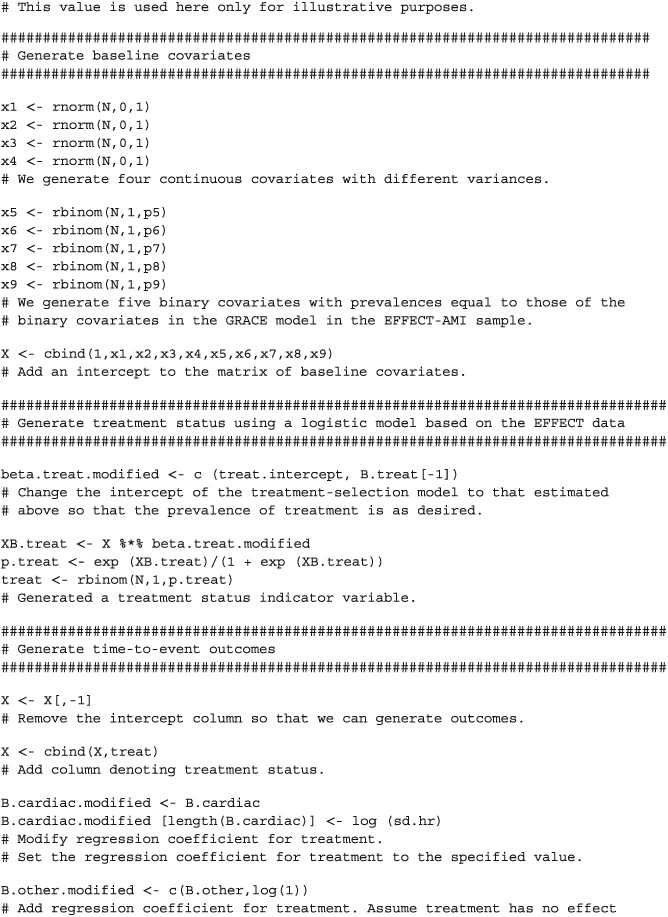
We used the analyses described in the previous subsection to inform the parameters used in the Monte Carlo simulations. When simulating event types and event times we used a method of indirect simulation described by Beyersmann et al.41 (Section 5.3.6), which in turn is based on an approach described by Fine and Gray.27 In doing so, one only needs to specify the underlying subdistribution hazard functions, and not the cause‐specific hazard functions.

3.2.1. Generation of baseline covariates

First, we simulated nine baseline covariates for each subject, such that the distribution of baseline covariates would be similar to that of the nine baseline covariates described above. Four of the simulated covariates were continuous and were drawn from independent standard normal distributions (since the four continuous covariates had been standardized to have mean zero and unit variance in the empirical analyses described above). Five of the simulated covariates were binary and were drawn from Bernoulli distributions with parameters equal to the five prevalences described in Section 3.1. We will let X₁,…, X₉ denote the nine simulated baseline covariates, where the first four are continuous and the last five are binary.

3.2.2. Generation of treatment status

We simulated a treatment status (Z_i) for each subject from a Bernoulli distribution: Z_i ∼ Be( p_treat), where logit( p_treat) =β₀ + β₁X₁ + ⋯ + β₉  X₉. The nine regression coefficients (β₁, …, β₉) for the nine baseline covariates in the treatment‐selection model were equal to the regression coefficients estimated in the empirical analyses described above. The intercept (β₀) was selected so as to induce a desired prevalence of treatment in the sample (see below for the target prevalences of treatment). A bisection approach, using a simulated dataset of size 1000000, was used to determine the intercept for the treatment‐selection model. We thus simulated a treatment status for each subject such that the relationship between the nine baseline covariates and the odds of treatment reflected what was observed in the EFFECT data described above. The only difference was that we modified the prevalence of treatment in the simulated data. This allowed us to examine the effect of prevalence of treatment on the performance of different methods for testing the equality of CIFs.

3.2.3. Generation of the event type that occurred (type 1 vs type 2 event) and the event time

Let the parameter p denote the proportion of subjects with covariates equal to zero who experience the event of interest as t → ∞. We generated event types using a method described in detail previously.37 In generating event types, we used the vector β ₁, obtained in Section 3.1, which is equal to the effect of the nine covariates on the incidence of cardiovascular death that was obtained from an analysis of the EFFECT data. We allowed p to take on a range of plausible values (see section below describing the design of the Monte Carlo simulations).

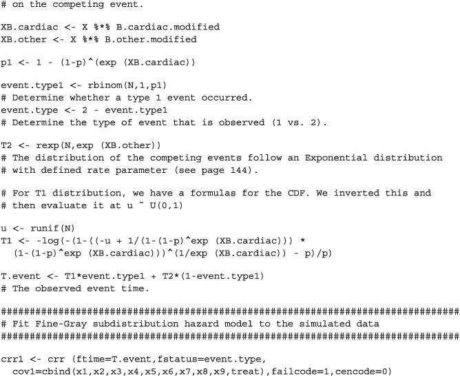
We simulated time‐to‐event outcomes conditional on the simulated failure type using a data‐generating process described in detail elsewhere.37 This data‐generating process is based on a method of indirect simulation described by Beyersmann et al.41 (Section 5.3.6), which in turn is based on an approach described by Fine and Gray.27 In simulating event times, we used the two vectors of regression parameters β ₁ and γ that were estimated above in the empirical analyses of the EFFECT data. In our simulations we did not introduce censoring, as we did not want to introduce another factor that could be varied (in addition to those factors described below).

3.3. Data generating process for generating data when there was a non‐null subdistribution hazard ratio

In our second set of simulations, we simulated data with a known subdistribution hazard ratio relating treatment status to the cumulative incidence of the primary outcome (ie, cardiovascular death). Baseline covariates, treatment status, and observed event types were simulated using methods identical to those described in the first set of simulations. However, when generating event times, the methods described above underwent minor modifications. For each simulated subject, the two potential outcomes were simulated: the potential outcome under control and the potential outcome under treatment42 (this will permit calculation of the true underlying marginal subdistribution hazard ratio; see subsequent section for a description of how this was accomplished). When generating event times, we used both the set of nine baseline covariates and the indicator variable denoting treatment status. Accordingly, we used the vector of regression coefficients β ₂, rather than β ₁ (ie, we used the regression coefficients that was obtained from regressing the subdistribution hazard of the primary outcome on the nine baseline covariates and on treatment status). However, β ₂ was modified so that the estimated regression coefficient for treatment was replaced with the logarithm of the desired conditional subdistribution hazard ratio. Thus, we were simulating data with a specified conditional subdistribution hazard ratio for treatment. As with the first set of simulations, we simulated the competing events so that they were not affected by treatment status. Each subject's observed event time was set to be equal to the potential outcome for the treatment that the subject actually received.

3.4. Statistical analyses in simulated datasets

3.4.1. Analyses in first set of simulations (under the null hypothesis of no difference in CIFs)

In each of the simulated datasets, we estimated the propensity score using logistic regression to regress the binary treatment variable on the nine baseline covariates. We then used propensity score matching to match treated and control subjects. We used two different matching algorithms. First, we used greedy nearest neighbor matching without replacement to match treated subjects to the control subject with the nearest propensity score.43 Second, we used caliper matching to match treated and control subjects on the logit of the propensity score using calipers of width equal to 0.2 of the standard deviation of the logit of the propensity score.44 We subsequently refer to these two matching methods nearest neighbor matching (NNM) and caliper matching, respectively.

Once a matched sample had been formed, we estimated CIFs for the primary outcome within the matched treated and matched control subjects separately. We then used four different methods to test the equality of the CIFs that were estimated in the matched treated and matched controls subjects: (i) Gray's test; (ii) the Wald test for a conventional Fine‐Gray model with a single covariate denoting treatment status (hereafter referred to as the naïve Fine‐Gray test); (iii) the Wald test for a univariate Fine‐Gray model that accounted for clustering within matched pairs (hereafter referred to as the clustered Fine‐Gray test); (iv) the Wald test from a univariate Fine‐Gray model that stratified on the matched pairs (hereafter referred to as the stratified Fine‐Gray test). All four methods were used in the matched sample. The first two methods do not account for the matched nature of the propensity‐score matched sample while the last two methods account for the matched nature of the propensity‐score matched sample. For each of the four methods, we extracted the p‐value for testing the equality of the two CIFs for the primary outcome.

3.4.2. Analyses in second set of simulations (estimation of subdistribution hazard ratios)

In each of the simulated datasets, we estimated the propensity score and created matched samples as in the first set of simulations. In each propensity‐score matched sample we fit three different subdistribution hazard models: (i) a conventional Fine‐Gray model with a single covariate denoting treatment status (hereafter referred to as the naïve Fine‐Gray model); (ii) a univariate Fine‐Gray model that accounted for clustering within matched pairs (hereafter referred to as the clustered Fine‐Gray model); (iii) a univariate Fine‐Gray model that stratified on the matched pairs (hereafter referred to as the stratified Fine‐Gray model). From each fitted model, we extracted the estimated regression coefficient (the log‐subdistribution hazard ratio) and the estimate of its standard error from the given model.

We also conducted a complementary conventional analysis in the full (unmatched sample). Using the full sample, we used a multivariable subdistribution hazard model to regress the subdistribution hazard of the primary outcome on the binary treatment indicator variable and the nine baseline covariates. From the fitted regression model, we extracted the estimated regression coefficient for the treatment effect variable.

3.5. Design of the Monte Carlo simulations

Our first set of Monte Carlo simulations employed a full factorial design in which the following three factors were allowed to vary: (i) the sample size of the simulated datasets; (ii) the prevalence of treatment in the sample; (iii) p (the proportion of subjects with covariates equal to zero who experience the primary event of interest as t → ∞). The sample size of the simulated datasets took five values: 1000, 2000, 3000, 4000, and 5000. The prevalence of treatment took five values: 0.05, 0.10, 0.15, 0.20, and 0.25. The parameter p was allowed to take on three values: from 0.25, 0.50, and 0.75. In doing so, we examined a range of plausible values for p, including a scenario in which the primary event was experienced by a higher proportion of subjects than the competing event and a scenario in which the converse was true. We thus examined 75 (5 × 5 × 3) different scenarios. We simulated 1000 datasets for each of the 75 scenarios.

Our second set of simulations also employed a full factorial design with one additional factor: the true adjusted subdistribution hazard ratio for treatment (adjusted for the effect of the nine baseline covariates). This was allowed to take four values: 1, 2, 3, and 4 (the first assumed no effect of treatment). The size of the simulated datasets was limited to 1000. We thus considered 60 (4 hazard ratios × 5 prevalences of treatment × 3 values of p) different scenarios. We simulated 1000 datasets for each of the 60 scenarios.

3.6. Summarizing the results of the simulations

In the first set of simulations, data were generated under the null hypothesis: treatment had no effect on the incidence of the primary outcome. In a given simulated dataset, we rejected the null hypothesis of no difference in CIFs if the estimated p‐value was less than or equal to 0.05. We estimated the empirical type I error rate as the proportion of the 1000 converged simulated datasets in which we rejected the null hypothesis of no difference in the CIFs between treated and control subjects in the matched sample.

In the second set of simulations, we determined the true underlying marginal subdistribution hazard ratio in each scenario as follows. First, we restricted the simulated sample to those subjects who were treated. In this restricted sample, we used a univariate subdistribution hazard model in which we regressed the two potential outcomes (whose simulation was described above) on an indicator variable denoting treatment status (thus, each subject contributed two records to this analysis, one record under treatment and one record under control) and determined the estimated log‐subdistribution marginal hazard ratio using a conventional Fine‐Gray subdistribution hazard model (as we were interested in only the estimated log‐subdistribution hazard ratio and not its standard error or statistical significance). This was done in each of the 1000 simulated datasets. Second, we determined the mean of the logarithm of the estimated marginal log‐subdistribution hazard ratio across the 1000 simulated datasets. The exponential of this quantity was used as the true underlying marginal subdistribution hazard ratio (when the conditional hazard ratio was equal to one, the true marginal hazard ratio was set equal to one45). We restricted this specific analysis to those subjects who were assigned to treatment as the target estimand when using propensity‐score matching is the average treatment effect in the treated (ATT). A similar approach has been used previously in the absence of competing risks.7, 11 This marginal subdistribution hazard ratio is the target estimand to which we will compare our estimates obtained using propensity‐score matching. Bias will be defined as the extent to which estimated marginal subdistribution hazard ratios deviate from this quantity (we refer to this target estimand as SDHR_marginal in the following formulas). The subsequent analyses used the matched samples constructed using the full simulated datasets. Then, for each of the three modeling approaches in the matched sample (naïve Fine‐Gray, clustered Fine‐Gray, and stratified Fine‐Gray), we computed the mean estimated log‐hazard ratio across the 1000 converged simulated datasets and then took the exponential of this quantity. The relative bias of each of the three estimation methods was defined as: $100\times \frac{{\text{SDHR}}_{\text{estimated}}-{\text{SDHR}}_{\text{marginal}}}{{\text{SDHR}}_{\text{marginal}}}$, where SDHR_estimated and SDHR_marginal denote the estimated and true marginal subdistribution hazard ratios, respectively.

For each of the three methods of estimation based on fitting a Fine‐Gray subdistribution hazard model in the matched sample, we obtained the estimated standard error of the estimated regression coefficient for the treatment indicator variable from the fitted subdistribution hazard model in each of the 1000 matched samples constructed in the simulated datasets. We computed the mean of the estimated standard errors across the 1000 simulated datasets. We then computed the standard deviation of the estimated regression coefficient for the treatment indicator variable across the 1000 simulated datasets. If the ratio of these two quantities is approximately equal to one, then the estimated standard error provides a reasonable approximation of the standard deviation of the sampling distribution of the estimated regression coefficients.

For the complementary conventional analysis that involved fitting a multivariable subdistribution hazard model in the full (unmatched) sample, we computed the relative bias in estimating both the underlying conditional subdistribution hazard ratio that was used in the data‐generating process and the marginal subdistribution hazard ratio that was determined above. When data were simulated under the null hypothesis of no treatment effect, we also determined the proportion of simulated samples in which we rejected the null hypothesis of no treatment effect using the multivariable subdistribution hazard model.

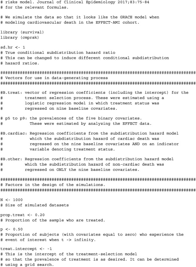
All simulations and statistical analyses were conducted using the R statistical software package46 (version 3.1.2). The subdistribution hazard models were fit using the crr function in the cmprsk package (version 2.2–7). The clustered subdistribution hazard models were fit using the crrc function in the crrSC package (version 1.1). The stratified subdistribution hazard models were fit using the censoring complete approach to fit the data using standard software for fitting a stratified Cox proportional hazards model (using the coxph function in the survival package for R).27 R code for simulating the time‐to‐event outcomes is provided in the Appendix.

4. MONTE CARLO SIMULATIONS: RESULTS

4.1. First set of simulations: Testing equality of CIFs under null hypothesis

The empirical type I error rates are reported in Figures 1 to 6. There is one figure for each of the 6 combinations of matching method (NNM vs caliper) and p (proportion of events that were type 1 events: 0.25, 0.50, and 0.75). Each figure consists of a series of dot charts. There are 25 horizontal lines, one for each combination of sample size (1000 to 5000 in increments of 1000) and prevalence of treatment (0.05 to 0.25 in increments of 0.05). On each horizontal line are four plotting symbols, representing the empirical type I error rates for the four methods of testing for equality of CIFs in the matched samples: (i) Gray's test; (ii) naïve Fine‐Gray test; (iii) clustered Fine‐Gray test; (iv) stratified Fine‐Gray test. Due to our use of 1000 converged simulated datasets for each scenario, any empirical type I error rate that is less than 0.0365 or greater than 0.0635 would be statistically significantly different from the nominal rate of 0.05 using a standard normal‐theory test. We have superimposed on each figure a vertical denoting an empirical type I error rate of 0.0365. Points to the left of this vertical denote scenarios and methods in which the empirical type I error rate was significantly different from the nominal rate of 0.05 (no empirical type I error rates exceeded 0.0635). In examining these figures, one observed that, in general, the use of Gray's test in the matched sample or the naïve Wald test from the conventional Fine‐Gray model fit in the matched sample tended to result in empirical type I error rates that were significantly lower than the advertised nominal rate. When using either Gray's test in the matched sample or the naïve Wald test from the conventional Fine‐Gray model fit in the matched sample, the empirical type I error rate was significantly lower than the advertised rate in either 68 (91%) or 69 (92%) of the 75 scenarios. In contrast, when using the clustered test or the stratified test in the matched samples, the empirical type I error rate was significantly lower than the advertised rate in only 13 (17%) (NNM and clustered Fine‐Gray), 16 (21%) (caliper matching with either the clustered or stratified Fine‐Gray model) or 19 (25%) (NNM and stratified Fine‐Gray) of the 75 scenarios.

Figure 1.

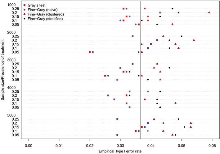
Empirical Type I error rates (Method = nearest neighbor matching & p = 0.25) [Colour figure can be viewed at http://wileyonlinelibrary.com]

Figure 6.

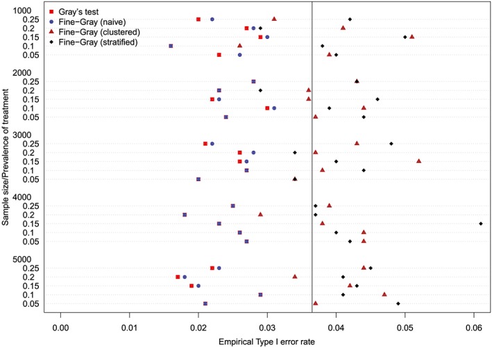
Empirical Type I error rates (Method = Caliper & p = 0.75) [Colour figure can be viewed at http://wileyonlinelibrary.com]

Figure 2.

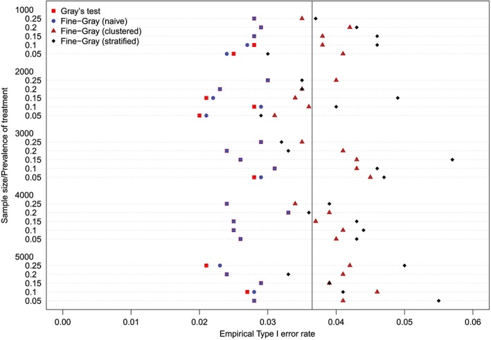
Empirical Type I error rates (Method = nearest neighbor matching & p = 0.5) [Colour figure can be viewed at http://wileyonlinelibrary.com]

Figure 3.

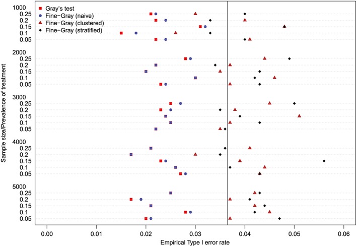
Empirical Type I error rates (Method = nearest neighbor matching & p = 0.75) [Colour figure can be viewed at http://wileyonlinelibrary.com]

Figure 4.

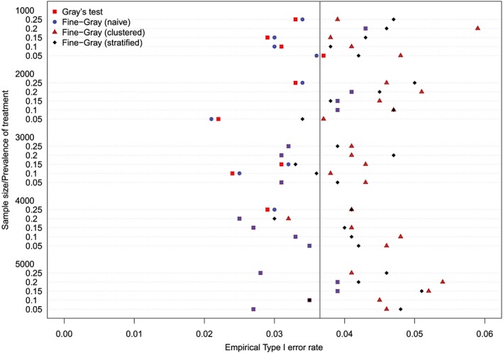
Empirical Type I error rates (Method = Caliper & p = 0.25) [Colour figure can be viewed at http://wileyonlinelibrary.com]

Figure 5.

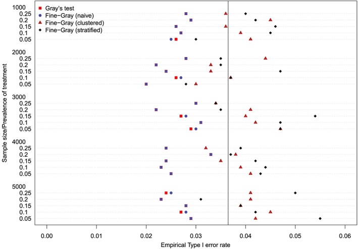
Empirical Type I error rates (Method = Caliper & p = 0.5) [Colour figure can be viewed at http://wileyonlinelibrary.com]

We fit a linear model in which we regressed the empirical type I error rate on the following factors: method of testing (Gray's test vs naïve Fine‐Gray Wald test vs Clustered Fine‐Gray Wald test vs Stratified Fine‐Gray Wald test), sample size, prevalence of treatment, p, and matching method (NNM vs caliper). All factors were treated as categorical variables. The empirical type I error rate differed across the four methods of testing (P < 0.0001), p (P < 0.0001), sample size (P = 0.023), prevalence of treatment (P = 0.027), while it did not differ across matching methods (P = 0.792). The empirical type I error rate for the naïve Fine‐Gray Wald test did not differ from that of Gray's test (P = 0.553), while the empirical type I error rates for the clustered and stratified Fine‐Gray model differed from that of Gray's test (P < 0.0001). The empirical type I error rate did not differ between the clustered and stratified approach (P = 0.281).

For comparative purposes, we also fit a univariate Fine‐Gray model in each simulated dataset and did not incorporate the propensity score (ie, no matching was performed). We then determined the proportion of simulated datasets in which we rejected the null hypothesis of equality of CIFs. The proportion of simulated datasets in which we rejected the null hypothesis ranged from 0.15 to 1 across the 75 scenarios (median: 0.87, 25^th, and 75^th percentiles: 0.63 and 0.982). Similar results were obtained for using Gray's test to test the equality of unadjusted CIFs in the full simulated dataset. Thus, failing to account for confounding resulted in incorrectly rejecting the null hypothesis of equality of CIFs in a large proportion of simulated datasets.

4.2. Second set of simulations: Estimation of subdistribution hazard ratios

The relative bias in the estimated marginal subdistribution hazard ratio is reported in Figures 7 to 10 (with one figure per true conditional subdistribution hazard ratio). The structure of these figures is similar to that of Figures 1 to 6. On each figure we have superimposed a vertical line denoting a relative bias of 0%. Estimation of the marginal subdistribution hazard ratio in the matched sample using the naïve Fine‐Gray model or the clustered Fine‐Gray model resulted in estimates with minimal bias (relative bias ranged from −3.6% to 0.8% across the different scenarios and matching methods). In contrast to this, estimation using the stratified Fine‐Gray model resulted in moderate bias (relative bias ranged from −1.8% to 25.2% across the different scenarios and matching methods). When the true conditional subdistribution hazard ratio was equal to one (which coincides with a marginal subdistribution hazard ratio of one), all methods resulted in essentially unbiased estimation of the underlying marginal subdistribution hazard ratio. The relative bias when using the stratified Fine‐Gray model increased with increasing magnitude of the true conditional subdistribution hazard ratio.

Figure 7.

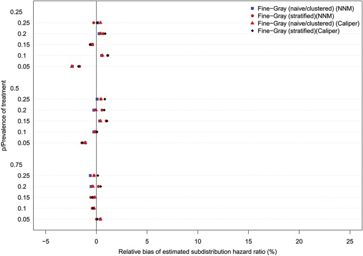
Relative bias (conditional subdistribution hazard ratio = 1). NNM, nearest neighbor matching [Colour figure can be viewed at http://wileyonlinelibrary.com]

Figure 10.

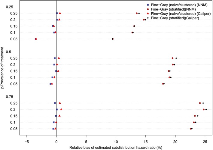
Relative bias (conditional subdistribution hazard ratio = 4). NNM, nearest neighbor matching [Colour figure can be viewed at http://wileyonlinelibrary.com]

Figure 8.

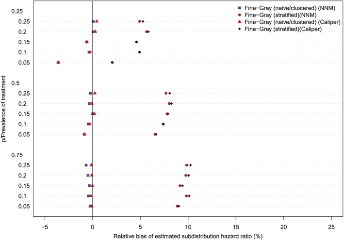
Relative bias (conditional subdistribution hazard ratio = 2). NNM, nearest neighbor matching [Colour figure can be viewed at http://wileyonlinelibrary.com]

Figure 9.

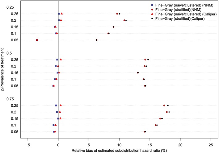
Relative bias (conditional subdistribution hazard ratio = 3). NNM, nearest neighbor matching [Colour figure can be viewed at http://wileyonlinelibrary.com]

Across the 60 scenarios, the mean relative bias in estimating the underlying conditional subdistribution hazard ratio when using a multivariable subdistribution hazard model in the full (unmatched) sample was 0.9% (range: −1.5% to 2.6%). When the true marginal subdistribution hazard ratio was equal to one (and therefore the true conditional subdistribution hazard ratio was also equal to one), the mean relative bias in estimating the marginal subdistribution hazard ratio when using a multivariable subdistribution hazard model in the full sample was −0.2% (range: −2.7% to 0.3%). However, when the true marginal subdistribution hazard ratio was larger than one, the mean relative bias in estimating the true marginal subdistribution hazard ratio when using a multivariable subdistribution hazard model in the full sample was 30.3% (range: 9.6% to 52.7%). In the 15 scenarios in which the true conditional subdistribution hazard ratio was equal to one (and therefore the true marginal subdistribution hazard ratio was also equal to one), the mean empirical type I error rate was 0.059 (range: 0.047 to 0.068). Due to our use of 1000 iterations per scenario, any empirical type I error rate that is less than 0.0365 or greater than 0.0635 would be statistically significantly different from the nominal rate of 0.05 based on a standard normal‐theory test. In four of the 15 scenarios (27%), the empirical type I error rate exceeded 0.0635 (range: 0.064 to 0.068).

The ratios between the mean estimated standard error and the standard deviation of the estimated log‐hazard ratios are reported in Figures 11 to 14 (with one figure per true conditional subdistribution hazard ratio). The structure of these figures is similar to that of Figures 7 to 10. On each figure, we have superimposed a vertical line denoting a ratio of one. Points to the right of this line indicate that in the given scenario, the given method resulted in estimated standard errors that over‐estimated the standard deviation of the sampling distribution of the regression coefficient. In examining these figures, it is apparent that the use of the naïve Fine‐Gray model in the matched sample tended to result in greater over‐estimation of the standard errors compared to when either a clustered or stratified Fine‐Gray model was used. When using the naïve Fine‐Gray model, the median ratio was 1.11 for both NNM and caliper matching across the 60 scenarios. When using the other methods, the median ratio ranged from 1.01 (stratified Fine‐Gray model with NNM or caliper matching) to 1.05 (clustered Fine‐Gray model with either NNM or caliper matching).

Figure 11.

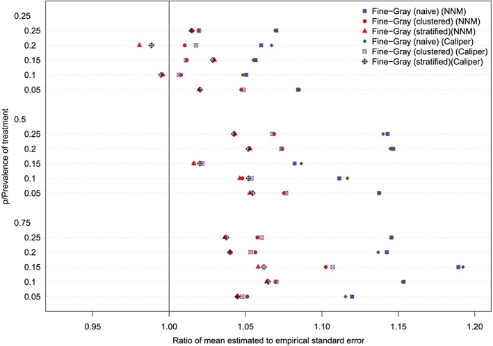
Standard error ratio (conditional subdistribution hazard ratio = 1). NNM, nearest neighbor matching [Colour figure can be viewed at http://wileyonlinelibrary.com]

Figure 14.

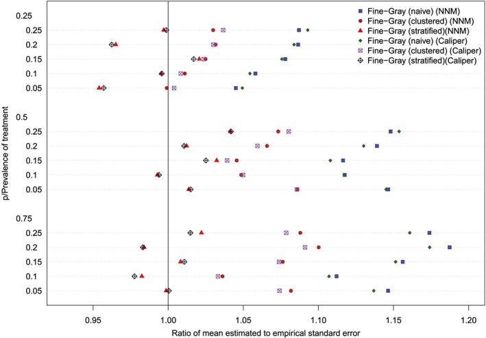
Standard error ratio (conditional subdistribution hazard ratio = 4). NNM, nearest neighbor matching [Colour figure can be viewed at http://wileyonlinelibrary.com]

Figure 12.

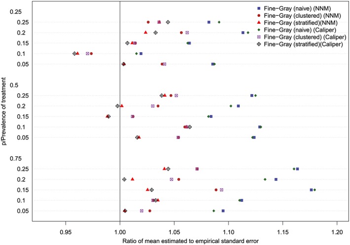
Standard error ratio (conditional subdistribution hazard ratio = 2). NNM, nearest neighbor matching [Colour figure can be viewed at http://wileyonlinelibrary.com]

Figure 13.

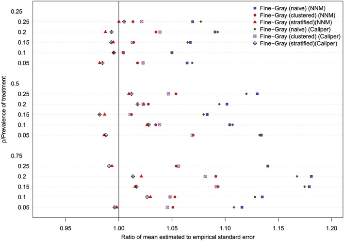
Standard error ratio (conditional subdistribution hazard ratio = 3). NNM, nearest neighbor matching [Colour figure can be viewed at http://wileyonlinelibrary.com]

5. CASE STUDY

We provide a case study to illustrate the application of propensity score matching in the presence of competing risks. We use the EFFECT data described in Section 2.1. The exposure of interest is statin prescribing at hospital discharge while the outcome is death within five years of follow‐up. Death was classified as due to cardiovascular causes or non‐cardiovascular causes.

5.1. Statistical analyses

Our first set of analyses consisted of conventional statistical analyses in which we fit a conditional cause‐specific hazard model and a conditional subdistribution hazard model in the full sample. In each of these models, the appropriate hazard function was regressed on an indicator variable denoting treatment status and the nine baseline covariates.

We then conducted a series of analyses using propensity‐score matching. We regressed the exposure, statin prescribing at hospital discharge, on the nine covariates from the GRACE mortality prediction model. We then created a matched sample using NNM on the propensity score. We created a second matched sample by matching treated and control subjects on the logit of the propensity score using calipers of width equal to 0.2 of the standard deviation of the logit of the propensity score. We used standardized differences to assess the balance in the nine baseline covariates between treated and control subjects in the matched samples.47

We estimated CIFs for cardiovascular death in the matched treated and matched control subjects in each of the two matched samples (the CIFs were estimated using the cuminc function from the cmprsk package for R). Based on the results of our simulations, we fit a clustered Fine‐Gray model to each of the two matched samples in which we regressed the subdistribution hazard for cardiovascular death on an indicator variable denoting treatment status. We also fit a cause‐specific hazard model in each matched sample in which we regressed the cause‐specific hazard of cardiovascular death on an indicator variable denoting treatment status. We fit a marginal model with a robust variance estimator to account for the matched nature of the sample.7

5.2. Results of empirical analyses

The means of the four continuous baseline covariates and the prevalences of the five dichotomous covariates in treated and control subjects in the full sample prior to matching are reported in the left half of Table 1. Standardized differences exceeded 0.10 for four of the baseline covariates (it has been suggested that standardized differences that are less than 0.10 denote negligible imbalance48). Thus, there is evidence of confounding, with the distribution of prognostically important baseline covariates differing between treated and control subjects.

Table 1.

Comparison of baseline characteristics between treated and control subjects in the case study

Variable	Before Matching			After Matching
	Control	Treated	Standardized	Control	Treated	Standardized
	(Mean/Prevalence)	(Mean/Prevalence)	Difference	(Mean/Prevalence)	(Mean/Prevalence)	Difference
Age	68.1	63.3	0.366	63.3	63.3	0.000
Heart Rate	84.6	81.6	0.127	81.4	81.6	0.007
Systolic BP	148.3	149.3	0.033	149.7	149.3	0.013
Creatinine	105.8	99.7	0.105	99.0	99.7	0.015
Previous AMI	20.8%	26%	0.124	25.5%	26%	0.011
Previous heart failure	4.6%	2.9%	0.089	3.0%	2.9%	0.004
Elevated cardiac enzymes	93.6%	95.1%	0.067	95.6%	95.1%	0.023
ST‐depression MI	47.2%	49.7%	0.050	49.0%	49.7%	0.014
In‐hospital PCI	0.8%	1.7%	0.079	1.4%	1.7%	0.024

The variables in the table are components of the GRACE risk score for predicting mortality in patients with acute coronary syndromes40

When we fit an adjusted subdistribution hazard ratio in the full (unmatched) sample, the estimated subdistribution hazard ratio for the treatment variable was 0.80 (95% confidence intervals: (0.71, 0.89)). Based on the direction of the subdistribution hazard ratio, we can infer that the incidence of cardiovascular death is lower in treated subjects than in control subjects. However, we are unable to make inferences about the magnitude of the difference in the cumulative incidence of cardiovascular between treated and control subjects. For the adjusted cause‐specific hazard model fit in the full sample, the estimated cause‐specific hazard ratio for the treatment variable was 0.76 (95% confidence interval: (0.68, 0.85)).

NNM resulted in the matching of all 3,359 treated subject to a control subject. Caliper matching resulted in the matching of 3353 (99.8%) treated subjects to a control subject (ie, only six treated subjects were excluded from the matched sample). Since the subsequent results were almost identical between the two matching methods, we present only the results for NNM. Excellent balance of baseline covariates between matched treated and matched control subjects was observed, with the absolute value of the standardized difference being less than 0.025 for all nine covariates (right half of Table 1).

The estimated CIFs in treated and control subjects are described in Figure 15. Post‐discharge incidence of cardiovascular death was lower in treated subjects than it was in control subjects. There was a statistically significant difference in the CIF curves between treated and control subjects (P = 0.00002 for Gray's test and the naïve Fine‐Gray model; P = 0.00001 for the clustered Fine‐Gray model; P = 0.00012 for the stratified Fine‐Gray model). The absolute decrease in the incidence of cardiovascular death due to discharge prescribing of statins was 0.015, 0.023, 0.028, 0.035, and 0.036 at 1, 2, 3, 4, and 5 years post‐discharge. The numbers needed to treat to avoid one death due to cardiovascular causes at 1, 2, 3, 4, and 5 years post‐discharge were 66, 44, 35, 28, and 28, respectively (the reciprocal of the absolute decrease in incidence).

Figure 15.

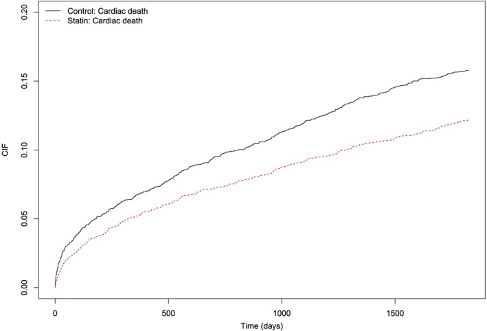
Cumulative incidence functions for cardiovascular death in nearest neighbor matching sample [Colour figure can be viewed at http://wileyonlinelibrary.com]

The estimated subdistribution hazard ratio from the clustered Fine‐Gray model was 0.76 (95% confidence interval: (0.67, 0.86)). Similarly to the hazard ratio from the usual Cox proportional hazard model without competing risks, one cannot provide a simple quantification of the relative change in the absolute risk of cardiovascular death due to statin prescribing.28 However, since the subdistribution hazard ratio is less than one, one can infer that the incidence of cardiovascular death is lower in treated subjects than in matched control subjects. It is for this reason that the NNT has been advocated for quantifying absolute treatment effects for survival data, both with and without competing risks.

The estimated cause‐specific hazard ratio was 0.75 (95% confidence interval: (0.66, 0.84)). Thus, statin prescribing at discharged decreased by 25% the rate of cardiovascular death in subjects who were currently alive.

We highlight that we have reported absolute treatment effects: absolute reductions in the cumulative incidence of cardiovascular death at 1, 2, 3, 4, and 5 years post‐discharge (along with the associated NNT). We have also reported the relative reduction in the rate of cardiovascular death in subjects who are currently event‐free (ie, who are currently alive). Thus, the reported analyses mirror what one would expect to be reported in an RCT with time‐to‐event outcomes. In contrast to this, the regression‐based analyses conducted in the full sample were restricted to reporting hazard ratios, which are relative measures of effect. As noted above, clinical commentators have argued that reporting relative measures of effects provides insufficient information to fully inform clinical decision making.15, 16, 17, 18, 19 Analyses based on the propensity score provide the information on both relative and absolute measures of treatment effect that are necessary to inform clinical decision making.

A further advantage of the use of propensity‐score matching in this context is that the analyst can clearly communicate the degree to which confounding due to measured covariates has been eliminated by matching on the propensity score. For instance, in examining Table 1, one observes that matching has resulted in the construction of a matched sample in which the distribution of baseline covariates is very similar between treated and control subjects. In contrast to this, when fitting a multivariable regression model in the full sample, it is difficult to assess the degree to which confounding has been adequately addressed and whether the outcomes regression model has been adequately specified.

Note that this case study is intended for illustrative purposes. Our intent was to illustrate the application of the methods discussed earlier. The paper is not intended to address the complex question of the efficacy of statins in this population.

6. DISCUSSION

In the current study we found that accounting for the matched nature of the propensity‐score matched sample resulted in empirical type I error rates that more accurately reflected the nominal type I error rates. Fitting a marginal model that accounted for matching or fitting a model that stratified on the matched pairs was preferable to the use of Gray's test or to using the Wald test from a naïve Fine‐Gray model fit in the matched sample. Similar results have been observed for other outcomes and models.7, 11, 33, 34 Thus, the current study contributes to the literature that demonstrates that statistical significance testing in propensity‐score matched samples should account for the matched nature of the sample. The reason that accounting for the matched nature of the sample is preferable to treating the matched treated and control subjects as independent is that subjects who have the same propensity score have observed baseline covariates that arise from the same multivariate distribution.1 Thus, matched treated and control subjects will, on average, have baseline covariates that are more similar than randomly selected treated and control subjects. In the presence of confounding, baseline covariates are associated with the outcome. Thus, matched subjects will, on average, have outcomes that are more similar than randomly selected treated and control subjects.

The results of our simulations showed that the marginal model that accounted for clustering and the model that stratified on the matched pairs tended to have similar empirical type I error rates when testing equality of CIFs in propensity‐score matched samples. This raises the question as to which of these two approaches should be used for testing the equality of CIFs in propensity‐score matched samples. Strictly speaking, the stratified approach uses a conditional model, in which one is conditioning on the matched pairs, while the clustered approach uses a marginal model. Propensity‐score matching permits estimation of the average treatment effect in the treated.2 In doing so, it is comparing outcomes between a population of treated subjects and an identical population of control subjects. Thus, the target estimand of propensity‐score matching is a marginal effect.21 The superior performance of the clustered Fine‐Gray model for estimating marginal subdistribution hazard ratios compared to that of the stratified Fine‐Gray model was observed in the second set of simulations. For this reason, we suggest that the clustered Fine‐Gray model be used for testing the equality of CIFs estimated in propensity‐score matched samples. However, it should be noted that under the null hypothesis, marginal and conditional effects coincide for non‐collapsible measures of effect, such as hazard ratios.45 Thus, when considered strictly for testing equality of CIFs, the two methods that account for matching should produce comparable results under the null hypothesis of equality of the CIFs. However, we recommend that the clustered Fine‐Gray model be used in practice, since it provides valid results under both the null and alternative hypotheses, which cannot be known in advance of analyzing the data.

When outcomes are time‐to‐event in nature, there are two different ways in which one can quantify the effects of treatments and interventions. First, one can estimate the relative effect of treatment on the hazard function. In doing so, one is examining whether the rate or intensity with which events occur differs between the treatment groups. Second, one can estimate the difference in survival functions between exposure groups. In the presence of competing risks, these two approaches correspond to whether the cause‐specific hazard function differs between treatment groups and whether the CIF differs between treatment groups. We would argue that a complete examination of the effect of treatment on time‐to‐event outcomes when using propensity‐score matching entails two sets of analyses: (i) estimation of CIFs within each of the treatment groups in the matched sample; (ii) estimation of the cause‐specific hazard ratio from a cause‐specific hazard regression model. The former can be complemented by estimation of a marginal subdistribution hazard ratio in the matched sample. For the latter, previous research has demonstrated that a robust variance estimator that accounts for the matched nature of the sample should be used.7 Our suggestion to estimate the effect of treatment on both the cause‐specific hazard and the CIF echoes the suggestion by Latouche et al35 that “both hazards and cumulative incidence be analyzed side by side, and that this is generally the most rigorous scientific approach to analyzing competing risks data.”

In the current study, we have focused solely on the use of propensity‐score matching in the presence of competing risks. We have not considered the use of IPTW using the propensity score, stratification on the propensity score, and covariate adjustment using the propensity score. Prior studies have shown that stratification and covariate adjustment using the propensity score induce less balance of baseline covariates than do matching and weighting using the propensity score.49 Furthermore, in the absence of competing risks, stratification and covariate adjustment using the propensity score result in biased estimation of both conditional and marginal hazard ratios.7, 8 Additionally, covariate adjustment using the propensity score requires the assumption that the outcomes model has been specified correctly. We did not examine the use of IPTW using the propensity score as the crr function in the cmprsk package for R does not currently support weights (similarly, the crrc function in the crrSC package does not currently support weights). Furthermore, a robust variance estimator should be used with IPTW to account for within‐subject correlation in outcomes induced by weighting.50, 51 As described by van der Wal,51,p.4‐5 “observations can have weights unequal to each other, which introduces clustering in the weighted dataset. When this is not taken into account, the standard error of the causal effect estimate could be underestimated.” The crr function also does not currently provide the option for a robust variance estimator. For these reasons, we did not consider IPTW using the propensity score, although this merits consideration in subsequent research.

Conventional regression adjustment and propensity score matching should not be seen as different approaches to addressing the same question. As evidenced by our simulations, these two approaches have different target estimands. A multivariable subdistribution hazard model has a conditional (or subject‐specific) target estimand, while matching on the propensity score has the average treatment effect in the treated (ATT), a marginal or population‐average effect, as its target estimand. The choice of analytic method should not be dictated by personal preference but by which method permits estimation of the desired estimand. A further difference between these two approaches is that multivariable regression adjustment limits the analyst to reporting relative measures of effect, whereas matching on the propensity score permits estimation of both relative and absolute measures of treatment effect. Using conventional regression analyses one can compute marginal estimates of treatment effects by averaging over the distributions of the covariates in the treated and untreated arms to obtain estimates of marginal treatment effects which are only conditional on treatment. This could be done by using the multivariable model to estimate a potential outcome for each subject under the treatment that was not received (eg, for treated subjects, an outcome under control could be generated from the fitted multivariable regression model).52 Outcomes under each treatment could then be summarized. For instance, a CIF could be estimated under control using all subjects (using the observed outcome for control subjects and the estimated outcome under control for treated subjects) and a CIF could be estimated under treatment using all subjects (using the estimated outcome under treatment for control subjects and the observed outcome for treated subjects). These indirect marginal treatment effects would not have a simple relationship with the treatment effect parameter in the multivariable regression model, but would still be valid. Of course, the analyses and resulting inferences would be much more complicated than what is done directly with propensity‐score matching when a univariate marginal model is fit to the matched sample. This is particularly true with survival data, where one would need to estimate the baseline hazard function in order to compute the marginal incidence function. Under a proportional hazards regression model, the resulting marginal (unconditional on non‐treatment covariates) incidence functions would not satisfy the proportional hazards assumption, making interpretation challenging. Furthermore, testing the statistical significance of the treatment effect using a multivariable regression model will not necessarily produce valid inferences about the significance of the marginal treatment effect. This occurs because the marginal treatment effect may be null even when the conditional treatment effect is non‐null.

There are certain limitations to the current study. First, our conclusions were based on Monte Carlo simulations. The design of these simulations was based on an analysis of empirical data, so that the simulations would reflect what was observed in a specific clinical setting. However, it is possible that different conclusions would be observed under a different data‐generating process. The current study reflects much of the current research on the propensity score methods, in which simulations, rather than mathematical derivations are employed.7, 8, 9, 11, 33, 34, 43, 44, 53, 54, 55, 56, 57, 58, 59, 60, 61, 62, 63 Second, our simulations did not incorporate censoring. Incorporating censoring would have required the addition of a much larger number of scenarios, as we used a full factorial design with 75 different scenarios in the first set of simulations and 60 different scenarios in the second of simulations. However, this issue merits examination in subsequent research.

In conclusion, when using propensity‐score matching in the presence of competing risks, analysts should estimate both the absolute and relative effects of treatment. Estimation of absolute treatment effects should incorporate estimation of the CIF in matched treated and matched control subjects. A marginal subdistribution hazard model that accounts for the matched nature of the sample can be used to test the equality of the CIFs between treatment groups and estimate the subdistribution hazard ratio for the effect of treatment on the cumulative incidence function. Relative effects of treatment can be estimated using a cause‐specific hazard model to regress the cause‐specific hazard of the primary outcome on an indicator variable denoting treatment status.

APPENDIX 1.

R CODE FOR SIMULATING COMPETING RISKS DATA

Austin PC, Fine JP. Propensity‐score matching with competing risks in survival analysis. Statistics in Medicine. 2019;38:751–777. 10.1002/sim.8008

REFERENCES

- 1. Rosenbaum PR, Rubin DB. The central role of the propensity score in observational studies for causal effects. Biometrika. 1983;70(1):41‐55. [Google Scholar]
- 2. Austin PC. An introduction to propensity‐score methods for reducing the effects of confounding in observational studies. Multivar Behav Res. 2011;46(3):399‐424. 10.1080/00273171.2011.568786 [DOI] [PMC free article] [PubMed] [Google Scholar]
- 3. Austin PC. Propensity‐score matching in the cardiovascular surgery literature from 2004 to 2006: a systematic review and suggestions for improvement. J Thorac Cardiovasc Surg. 2007;134(5):1128‐1135. [DOI] [PubMed] [Google Scholar]
- 4. Austin PC. A critical appraisal of propensity‐score matching in the medical literature between 1996 and 2003. Statist Med. 2008;27(12):2037‐2049. [DOI] [PubMed] [Google Scholar]
- 5. Austin PC. A report card on propensity‐score matching in the cardiology literature from 2004 to 2006: a systematic review and suggestions for improvement. Circ Cardiovasc Qual Outcomes. 2008;1:62‐67. [DOI] [PubMed] [Google Scholar]
- 6. Austin PC, Manca A, Zwarenstein M, Juurlink DN, Stanbrook MB. A substantial and confusing variation exists in handling of baseline covariates in randomized controlled trials: a review of trials published in leading medical journals. J Clin Epidemiol. 2010;63(2):142‐153. 10.1016/j.jclinepi.2009.06.002 [DOI] [PubMed] [Google Scholar]
- 7. Austin PC. The performance of different propensity score methods for estimating marginal hazard ratios. Statist Med. 2013;32(16):2837‐2849. 10.1002/sim.5705 [DOI] [PMC free article] [PubMed] [Google Scholar]
- 8. Austin PC, Grootendorst P, Normand SL, Anderson GM. Conditioning on the propensity score can result in biased estimation of common measures of treatment effect: a Monte Carlo study. Statist Med. 2007;26(4):754‐768. [DOI] [PubMed] [Google Scholar]
- 9. Austin PC, Schuster T. The performance of different propensity score methods for estimating absolute effects of treatments on survival outcomes: a simulation study. Stat Methods Med Res. 2016;25(5):2214‐2237. 10.1177/0962280213519716 [DOI] [PMC free article] [PubMed] [Google Scholar]
- 10. Austin PC. The use of propensity score methods with survival or time‐to‐event outcomes: reporting measures of effect similar to those used in randomized experiments. Statist Med. 2014;33(7):1242‐1258. 10.1002/sim.5984 [DOI] [PMC free article] [PubMed] [Google Scholar]
- 11. Gayat E, Resche‐Rigon M, Mary JY, Porcher R. Propensity score applied to survival data analysis through proportional hazards models: a Monte Carlo study. Pharm Stat. 2012;11(3):222‐229. 10.1002/pst.537 [DOI] [PubMed] [Google Scholar]
- 12. Austin PC, Lee DS, Fine JP. Introduction to the analysis of survival data in the presence of competing risks. Circulation. 2016;133(6):601‐609. 10.1161/CIRCULATIONAHA.115.017719 [DOI] [PMC free article] [PubMed] [Google Scholar]
- 13. Putter H, Fiocco M, Geskus RB. Tutorial in biostatistics: competing risks and multi‐state models. Statist Med. 2007;26(11):2389‐2430. 10.1002/sim.2712 [DOI] [PubMed] [Google Scholar]
- 14. Lau B, Cole SR, Gange SJ. Competing risk regression models for epidemiologic data. Am J Epidemiol. 2009;170(2):244‐256. 10.1093/aje/kwp107 [DOI] [PMC free article] [PubMed] [Google Scholar]
- 15. Cook RJ, Sackett DL. The number needed to treat: a clinically useful measure of treatment effect. Br Med J. 1995;310(6977):452‐454. [DOI] [PMC free article] [PubMed] [Google Scholar]
- 16. Laupacis A, Sackett DL, Roberts RS. An assessment of clinically useful measures of the consequences of treatment. N Engl J Med. 1988;318(26):1728‐1733. [DOI] [PubMed] [Google Scholar]
- 17. Jaeschke R, Guyatt G, Shannon H, Walter S, Cook D, Heddle N. Basic statistics for clinicians: 3. Assessing the effects of treatment: measures of association. Can Med Assoc J. 1995;152(3):351‐357. [PMC free article] [PubMed] [Google Scholar]
- 18. Schechtman E. Odds ratio, relative risk, absolute risk reduction, and the number needed to treat–which of these should we use? Value Health. 2002;5(5):431‐436. [DOI] [PubMed] [Google Scholar]
- 19. Sinclair JC, Bracken MB. Clinically useful measures of effect in binary analyses of randomized trials. J Clin Epidemiol. 1994;47(8):881‐889. [DOI] [PubMed] [Google Scholar]
- 20. Austin PC, Laupacis A. A tutorial on methods to estimating clinically and policy‐meaningful measures of treatment effects in prospective observational studies: a review. Int J Biostat. 2011;7(1):1‐32 10.2202/1557-4679.1285 [DOI] [PMC free article] [PubMed] [Google Scholar]
- 21. Rosenbaum PR. Propensity Score In: Armitage P, Colton T, eds. Encyclopedia of Biostatistics. Boston, MA: Wiley; 2005:4267‐4272. [Google Scholar]
- 22. Dorn HF. Philosophy of inference from retrospective studies. Am J Public Health. 1953;43:677‐683. [DOI] [PMC free article] [PubMed] [Google Scholar]
- 23. Rubin DB. Matched Sampling for Causal Effects. New York, NY: Cambridge University Press; 2006. [Google Scholar]
- 24. BMJ Publishing Group . Article types and preparation. http://www.bmj.com/about-bmj/resources-authors/article-types. Accessed March 5, 2018.
- 25. Altman DG, Andersen PK. Calculating the number needed to treat for trials where the outcome is time to an event. BMJ. 1999;319(7223):1492‐1495. [DOI] [PMC free article] [PubMed] [Google Scholar]
- 26. Gouskova NA, Kundu S, Imrey PB, Fine JP. Number needed to treat for time‐to‐event data with competing risks. Statist Med. 2014;33(2):181‐192. 10.1002/sim.5922 [DOI] [PubMed] [Google Scholar]
- 27. Fine JP, Gray RJ. A proportional hazards model for the subdistribution of a competing risk. J Am Stat Assoc. 1999;94:496‐509. [Google Scholar]
- 28. Austin PC, Fine JP. Practical recommendations for reporting Fine‐Gray model analyses for competing risk data. Stat Med. 2017;36(27):4391‐4400. 10.1002/sim.7501 [DOI] [PMC free article] [PubMed] [Google Scholar]
- 29. Gray RJ. A class of K‐sample tests for comparing the cumulative incidence of a competing risk. Ann Stat. 1988;16:1141‐1154. [Google Scholar]
- 30. Schafer JL, Kang J. Average causal effects from nonrandomized studies: a practical guide and simulated example. Psychol Methods. 2008;13(4):279‐313. [DOI] [PubMed] [Google Scholar]
- 31. Zhou B, Fine J, Latouche A, Labopin M. Competing risks regression for clustered data. Biostatistics. 2012;13(3):371‐383. 10.1093/biostatistics/kxr032 [DOI] [PMC free article] [PubMed] [Google Scholar]
- 32. Zhou B, Latouche A, Rocha V, Fine J. Competing risks regression for stratified data. Biometrics. 2011;67(2):661‐670. 10.1111/j.1541-0420.2010.01493.x [DOI] [PMC free article] [PubMed] [Google Scholar]
- 33. Austin PC. Type I error rates, coverage of confidence intervals, and variance estimation in propensity‐score matched analyses. Int J Biostat. 2009;5(1):1557‐4679. 10.2202/1557-4679.1146 [DOI] [PMC free article] [PubMed] [Google Scholar]
- 34. Austin PC. Comparing paired vs non‐paired statistical methods of analyses when making inferences about absolute risk reductions in propensity‐score matched samples. Statist Med. 2011;30(11):1292‐1301. [DOI] [PMC free article] [PubMed] [Google Scholar]
- 35. Latouche A, Allignol A, Beyersmann J, Labopin M, Fine JP. A competing risks analysis should report results on all cause‐specific hazards and cumulative incidence functions. J Clin Epidemiol. 2013;66(6):648‐653. [DOI] [PubMed] [Google Scholar]
- 36. Franklin JM, Schneeweiss S, Polinski JM, Rassen JA. Plasmode simulation for the evaluation of pharmacoepidemiologic methods in complex healthcare databases. Comput Stat Data Anal. 2014;72:219‐226. 10.1016/j.csda.2013.10.018 [DOI] [PMC free article] [PubMed] [Google Scholar]
- 37. Austin PC, Allignol A, Fine JP. The number of primary events per variable affects estimation of the subdistribution hazard competing risks model. J Clin Epidemiol. 2017;83:75‐84. 10.1016/j.jclinepi.2016.11.017 [DOI] [PubMed] [Google Scholar]
- 38. Tu JV, Donovan LR, Lee DS, et al. Effectiveness of public report cards for improving the quality of cardiac care: the EFFECT study: a randomized trial. JAMA. 2009;302(21):2330‐2337. [DOI] [PubMed] [Google Scholar]
- 39. Tu JV, Chu A, Donovan LR, et al. The cardiovascular health in ambulatory care research team (CANHEART): using big data to measure and improve cardiovascular health and healthcare services. Circ Cardiovasc Qual Outcomes. 2015;8(2):204‐212. 10.1161/CIRCOUTCOMES.114.001416 [DOI] [PubMed] [Google Scholar]
- 40. Eagle KA, Lim MJ, Dabbous OH, et al. A validated prediction model for all forms of acute coronary syndrome: estimating the risk of 6‐month postdischarge death in an international registry. JAMA. 2004;291(22):2727‐2733. [DOI] [PubMed] [Google Scholar]
- 41. Beyersmann J, Allignol A, Schumacher M. Competing Risks and Multistate Models with R. New York, NY: Springer; 2012. [Google Scholar]
- 42. Rubin DB. Estimating causal effects of treatments in randomized and nonrandomized studies. J Educ Psychol. 1974;66(5):688‐701. [Google Scholar]
- 43. Austin PC. A comparison of 12 algorithms for matching on the propensity score. Statist Med. 2014;33(6):1057‐1069. [DOI] [PMC free article] [PubMed] [Google Scholar]
- 44. Austin PC. Optimal caliper widths for propensity‐score matching when estimating differences in means and differences in proportions in observational studies. Pharm Stat. 2011;10(2):150‐161. [DOI] [PMC free article] [PubMed] [Google Scholar]
- 45. Gail MH, Wieand S, Piantadosi S. Biased estimates of treatment effect in randomized experiments with nonlinear regressions and omitted covariates. Biometrika. 1984;71(3):431‐444. 10.1093/biomet/71.3.431 [DOI] [Google Scholar]
- 46. RC Team . R: a language and environment for statistical computing. Vienna, Austria: R Foundation for Statistical Computing; 2005. https://www.r-project.org/ [Google Scholar]
- 47. Austin PC. Balance diagnostics for comparing the distribution of baseline covariates between treatment groups in propensity‐score matched samples. Statist Med. 2009;28(25):3083‐3107. [DOI] [PMC free article] [PubMed] [Google Scholar]
- 48. Mamdani M, Sykora K, Li P, et al. Reader's guide to critical appraisal of cohort studies: 2. Assessing potential for confounding. Br Med J. 2005;330(7497):960‐962. [DOI] [PMC free article] [PubMed] [Google Scholar]
- 49. Austin PC. The relative ability of different propensity score methods to balance measured covariates between treated and untreated subjects in observational studies. Med Decis Making. 2009;29(6):661‐677. [DOI] [PubMed] [Google Scholar]
- 50. Hernan MÁ, Brumback B, Robins JM. Marginal structural models to estimate the causal effect of zidovudine on the survival of HIV‐positive men. Epidemiology. 2000;11(5):561‐570. [DOI] [PubMed] [Google Scholar]
- 51. van der Wal WM, Geskus RB. Ipw: an R package for inverse probability weighting. J Stat Softw. 2011;43(13):1‐23. [Google Scholar]
- 52. Imbens GW. Nonparametric estimation of average treatment effects under exogeneity: a review. Rev Econ Stat. 2004;86(1):4‐29. [Google Scholar]
- 53. Austin PC, Grootendorst P, Anderson GM. A comparison of the ability of different propensity score models to balance measured variables between treated and untreated subjects: a Monte Carlo study. Statist Med. 2007;26(4):734‐753. [DOI] [PubMed] [Google Scholar]
- 54. Austin PC. Some methods of propensity‐score matching had superior performance to others: results of an empirical investigation and Monte Carlo simulations. Biom J J Math Methods Biosci. 2009;51(1):171‐184. [DOI] [PubMed] [Google Scholar]
- 55. Austin PC. The performance of different propensity‐score methods for estimating relative risks. J Clin Epidemiol. 2008;61(6):537‐545. [DOI] [PubMed] [Google Scholar]
- 56. Austin PC. The performance of different propensity score methods for estimating marginal odds ratios. Statist Med. 2007;26(16):3078‐3094. [DOI] [PubMed] [Google Scholar]
- 57. Austin PC. Statistical criteria for selecting the optimal number of untreated subjects matched to each treated subject when using many‐to‐one matching on the propensity score. Am J Epidemiol. 2010;172(9):1092‐1097. [DOI] [PMC free article] [PubMed] [Google Scholar]
- 58. Austin PC. The performance of different propensity‐score methods for estimating differences in proportions (risk differences or absolute risk reductions) in observational studies. Statist Med. 2010;29(20):2137‐2148. [DOI] [PMC free article] [PubMed] [Google Scholar]
- 59. Austin PC, Small DS. The use of bootstrapping when using propensity‐score matching without replacement: a simulation study. Statist Med. 2014;33(24):4306‐4319. 10.1002/sim.6276 [DOI] [PMC free article] [PubMed] [Google Scholar]
- 60. Austin PC. Double propensity‐score adjustment: a solution to design bias or bias due to incomplete matching. Stat Methods Med Res. 2017;26(1):201‐222. 10.1177/0962280214543508 [DOI] [PMC free article] [PubMed] [Google Scholar]
- 61. Austin PC, Stuart EA. The performance of inverse probability of treatment weighting and full matching on the propensity score in the presence of model misspecification when estimating the effect of treatment on survival outcomes. Stat Methods Med Res. 2017;26(4):1654‐1670. 10.1177/0962280215584401 [DOI] [PMC free article] [PubMed] [Google Scholar]
- 62. Austin PC, Stuart EA. Estimating the effect of treatment on binary outcomes using full matching on the propensity score. Stat Methods Med Res. 2017;26(6):2505‐2525. 10.1177/0962280215601134 [DOI] [PMC free article] [PubMed] [Google Scholar]
- 63. Franklin JM, Eddings W, Austin PC, Stuart EA, Schneeweiss S. Comparing the performance of propensity score methods in healthcare database studies with rare outcomes. Statist Med. 2017;36(12):1946‐1963. 10.1002/sim.7250 [DOI] [PubMed] [Google Scholar]