Characterization of Age-Based Trends to Identify Chemical Biomarkers of Higher Levels in Children

Abstract

Background:

Chemical biomarker concentrations are driven by complex interactions between chemical use patterns, exposure pathways, and toxicokinetic parameters such as biological half-lives. Criteria to differentiate legacy from current exposures are helpful for interpreting variation in age-based and time trends of chemical exposure and identifying chemicals to which children are highly exposed. A systematic approach is needed to study temporal trends for a wide range of chemicals in the US population.

Objectives:

Using NHANES data on measured biomarker concentrations for 141 chemicals from 1999–2014, we aim to 1) understand the influence of temporal determinants, in particular time trends, biological half-lives, and restriction dates on age-based trends, 2) systematically define an age-based pattern to identify chemicals with ongoing and high exposure in children, and 3) characterize how age-based trends for six Per- and Polyfluoroalkyl Substances (PFASs) are changing over time.

Methods:

We performed an integrated analysis of biological half-lives and restriction dates, compared distributions of chemical biomarker concentrations by age group, and then applied a series of regression models to evaluate the linear $({\beta }_{age})$ and nonlinear $({\beta }_{ag{e}^2})$ relationships between age and chemical biomarker levels.

Results:

For restricted chemicals, a minimum persistence of 1 year in the human body is needed to observe substantial differences between less exposed young population and historically exposed adults. We define a metric $({\beta }_{ag{e}^2}/{\beta }_{age}>\frac{1}{26.9})$ that identifies several phthalates, brominated flame retardants, pesticides, and metals such as lead and tungsten to reflect elevated and ongoing exposures in children. While a substantial reduction in children’s exposures was reflected in PFOS and PFOA, levels of PFNA and PFHxS in children were higher in 2013–2014 compared to those in 1999–2000.

Conclusions:

Integrating a series of regression models with systemized stratified analyses by age group enabled us to define an age-based pattern to identify chemicals that are of higher level in children.

1. INTRODUCTION

Characterizing an individual’s exposome requires understanding their lifelong chemical exposures, including how chemical exposures change over time and by age. Studies using population-level chemical biomonitoring data have observed a variety of chemical-specific time and age trends. Persistent chemicals such as polychlorinated biphenyls (PCBs) tend to show a strong decline over time and differentiated exposure patterns across life stages, which are linked to chemical persistency and changes in legislation (Quinn and Wania 2012; Xue et al. 2014). Relative to PCB exposures which derive mainly from the diet, characterizing exposures to chemicals in consumer products, such as phthalates, are more complex, since these chemicals are used in a range of products with varying usage patterns. As a result, very different age-based and temporal patterns can be observed even within the same chemical family. For instance, urinary concentrations of mono-ethyl phthalate, mono-n-butyl phthalate, mono-benzyl phthalate, and metabolites of di(2-ethylhexyl) phthalate showed a decline, whereas mono-isobutyl phthalate, mono(3-carboxypropyl) phthalate, mono-carboxyoctyl phthalate, and mono-carboxynonyl phthalate increased from 2001 to 2010, implying that the latter phthalates may be substitutes for the former (Zota et al. 2014). Similar trends can be observed in biomonitoring data for per- and polyfluoroalkyl substances (PFASs), such as perfluorooctane sulfonate (PFOS) and perfluorooctanoate (PFOA), where differences in population concentrations manifested following restrictions in 2000–2002 (Calafat et al. 2007; Kato et al. 2011). The exposure patterns of other PFASs from treated consumer products (Trudel et al. 2008), water (Gyllenhammar et al. 2018; Mondal et al. 2012), and food contamination (Schecter et al. 2010) are not as well understood and evoke the need to study how age-based trends for these substances are changing over time (Gomis et al. 2017). While many studies have used biomonitoring data to identify a variety of chemical-specific time and age trends, expanding these analyses to a broader set of chemicals and chemical classes will enable us to understand the drivers behind these age-based trends.

To better understand the relationship between chemical biomarker levels and age, several mechanistic models have been developed to investigate the potential determinants. These models have studied age relationships for specific chemical classes such as PCBs (Quinn and Wania 2012; Ritter et al. 2011), dioxins (Jolliet et al. 2008), and selected PFASs (Gomis et al. 2017; Wong et al. 2014), with most considering dietary exposure pathways. These models have enabled the identification of key potential determinants such as biological half-lives, restriction dates, and change of intake with age as important factors in understanding age-based trends. However, such models have mostly been applied to dietary exposures for persistent chemicals and require substantial amount of data on age-based exposure patterns, chemical properties, and chemical usage. Such stipulations make a systematic application across a broad set of chemical classes and exposure pathways complex and challenging. Thus, an overarching statistical approach anchored in biomonitoring data would complement mechanistic approaches by allowing us to screen age-based trends and main determinants across a larger number of chemicals, chemical classes and (even unknown) product usage, to identify subpopulations at risk of high exposure.

Compared to adults, children are particularly susceptible to toxicant exposures due to factors such as higher metabolic rate (Shimokata and Kuzuya 1993; Speakman 2005), rapid growth, development of organs and tissues (Services 2012), and behaviors associated with normal development such as crawling (Just et al. 2015), mouthing (Tsou et al. 2015; Xu et al. 2010), and playing (Kumar and Pastore 2007). For example, higher concentrations of polybrominated diphenyl ethers (PBDEs) in younger individuals were attributed to lifestyle and activity differences (Sjödin et al., 2008). Due to their increased susceptibility, it is imperative to identify chemicals to which children are highly exposed. Comparing geometric means of chemical levels across age groups enables the identification of chemicals that are higher in children (Jl et al. 1994; Richter et al. 2009; Silva et al. 2004). Such approaches do not account for confounders, however, nor do they inform the influence of potential determinants on age-based trends. There is a need integrate data on biological half-lives and restriction dates with cross-sectional biomonitoring data to understand age patterns and systematically identify ongoing exposures in children.

While progress has been made to characterize temporal trends for a few chemical classes, an overarching screening approach has yet to be developed to systematically study age-based and temporal trends of biomarker data in context with temporal determinants such as half-lives and restriction dates for a wide range of chemicals in the US population. In this study, we therefore applied a systematic approach through a series of regression models to characterize chemical specific age-based patterns and identify highly exposed subpopulations for a broad set of 141 chemical biomarkers from a 1999–2014 sample of the US population. More specifically, our objectives were to 1) understand the influence of temporal determinants on age-based trends, in particular time trends, biological half-lives, and restriction dates, 2) systematically define an age-based pattern of concern to identify chemicals of ongoing and high exposures in the younger population, and 3) conduct a targeted analysis of six PFASs to characterize how age-based trends of these substances are changing over time.

2. MATERIAL AND METHODS

The approach integrates four types of data: a large dataset of biomarker concentrations for multiple chemicals in a large sample of the US population, the corresponding demographic factors for the studied population, a dataset of human biological half-lives for the observed chemicals, and a dataset describing the year and type of restrictions imposed on the production, emission, sale or use of products containing these substances, if applicable.

2.1. Study Population

Since 1999, the Centers for Disease Control (CDC) has conducted the continuous National Health and Nutrition Examination Survey (NHANES) to collect cross-sectional data on demographic, socioeconomic, dietary, and health-related characteristics in the US population. For this analysis, we combined data from the chemical biomarker and demographic datasets between years 1999–2014 for an initial number of 82,091 participants. We then excluded participants for which corresponding data on chemical biomarkers do not exist (n = 7,149), resulting in a sample size of 74,942 study participants. On a chemical specific basis, we also excluded participants with missing information on any of the following covariates: age, NHANES cycles, sex, race/ethnicity, poverty income ratio, cotinine levels, and urinary creatinine. These exclusion and inclusion criteria are detailed in Figure 1.

Figure 1.

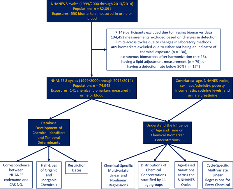
Schematic description of the process to curate chemical biomarker measurements and of the analytical methods used to identify temporal variations in biomarker levels.

2.2. Chemical Biomarker Measurements

We define chemical biomarker as an indicator of environmental exposure that can be measured in blood, serum, or urine. Table S1 presents brief descriptions of the laboratory techniques, while details of the procedure can be assessed through their corresponding references. We replaced all measurements below the limit of detection (LOD) with the LOD divided by the square root of 2, as recommended by the CDC (CDC 2009) to produce reasonably unbiased means and standard deviations (Hornung and Reed 1990). At times, NHANES identified a problem of interference from molybdenum oxide that resulted in corrected concentration of urinary cadmium recorded as 0 ng/mL (NCHS 2005a, b). Log-transforming such data would be undefined, therefore such measurements were replaced with the LOD divided by the square root of 2 if the participant’s urinary cadmium level was under the LOD or otherwise excluded. We calculated detection frequencies for each chemical biomarker (SI, Table S2) and excluded biomarkers with detection frequencies of 50% or less (n = 173). Across the NHANES cycles, improvements in laboratory technology can change the LOD and thus influence changes in detection frequencies by NHANES cycle. To prevent such influence, we calculated detection frequencies by NHANES cycle (SI, Table S3) for each chemical biomarker and excluded measurements that showed drastic changes in the LOD (Table S4) and detection frequencies over time (Figure 1). For instance, percentages of participants with PCB 196 measurements above LOD for Cycle 2 and Cycle 3 are 37.8% and 86.7%, respectively, and the LOD for Cycle 2 and Cycle 3 were 10.50 ng/g and 0.40 ng/g, respectively. As such, measurements from Cycle 2 for PCB 196 were excluded. Measurements from given cycles for all PCBs, Dioxins, and Furans along with 2-(N-methyl-PFOSA) acetate, 2,4-D, Paranitrophenol, and 1-pyrene (n = 134,453) were therefore also excluded based on this criteria (SI, Table S5). We also excluded biomarkers that are not indicative of exposure (n = 30). We preferred lipid adjusted measurements for biomarkers indicated by 7- or 8-letter NHANES codename ending in “L” or “LA,” respectively, for which NHANES provided both lipid-adjusted and non-lipid adjusted measurements, and excluded non-lipid adjusted chemical biomarkers (n = 79). Finally, transition from the early to recent NHANES cycles resulted in differences in NHANES chemical codenames, which we corrected to reflect a unique codename for each biomarker (n = 22). The final dataset for analysis consisted of 141 chemical biomarkers from 16 different classes.

2.3. Half-Lives of Organic and Inorganic Substances in Humans

The biological half-life of a chemical is an important factor to explain differences in chemical biomarker levels across the life-stages (Quinn and Wania 2012). To determine a set of relevant half-lives, we first developed a table of NHANES codenames and corresponding CAS No. for each chemical biomarker (SI, Table S7). We then matched metabolite biomarkers to their corresponding parent compounds. For biomarkers that are metabolites of several parent compounds, we developed the composite half-life by summing the half-life of the metabolite with the maximum half-life of the corresponding parent substances. This assumes the parent substance or compartment with the highest persistence drives the persistency of the metabolic biomarker. We searched a database of empirically-based whole body elimination half-lives and identified 39 chemicals on the list (Arnot et al. 2014). For an NHANES chemical biomarker that is a mixture of two substances, i.e. m-/p-Xylene, we applied the average of the substance’s half-life. Thirty nine of the 118 organic chemicals in this study have empirically-based whole body elimination half-lives available in the OECD QSAR ToolBox (https://www.qsartoolbox.org/). Since estimated persistency of PFASs showed high variability with estimates up to 220 years, empirically based half-lives were selected from literature for this chemical class (SI, Text S1 and Table S8). For organic chemicals that are not in the empirical database, the total elimination (intrinsic) half-life was predicted using a screening-level Quantitative Structure-Activity Relationship (QSAR) (Arnot et al. 2014). The model is a fragment-based QSAR that was developed and validated following OECD QSAR guidance (OECD 2004, 2014). Since these QSARs are only applicable to organic substances, we identified the half-lives of inorganic substances in humans through a review (SI, Table S9). In selecting literature half-lives, we preferred 1) human half-lives over those from animals, 2) half-lives from animal species that are anatomically similar to humans if human data were not available, and 3) slower elimination kinetics over rapid kinetics. We selected the maximum half-life for 1) inorganic chemicals that have multiple half-lives for a given biological compartment, and for 2) chemicals with half-lives available for multiple biological compartments, e.g. body, bones, blood, or lungs. SI Table S12 tabulates the methods used to find or estimate half-life for each chemical biomarker.

2.4. Restriction Dates

It has been suggested that the time-lapse between a chemical’s restriction date and sample collection date is an important contributor to biomarker concentration time trends and age-based differentiations (Quinn and Wania 2012). To investigate this, we developed a database of restriction dates (years) in US commerce through an extensive review (SI, Table S10). Some chemicals have several reported restriction dates, in particular those that were restricted from different products in different years, such as lead. Note that some chemicals were restricted in certain applications but not in others. For instance, the use of lead was banned in paint (Fowler 2008) and gasoline (Newell and Rogers 2003), but it is still used in cosmetic products (FDA 2018) and plumbing (US EPA 2011, 2017). Also, some chemicals have been gradually phased out over several years, such as PFASs. For chemicals with dates recorded as a range, and for which we were unable to determine the relative importance of a given year, we applied the mean year. When there are several dates associated with a chemical biomarker, we applied the latest date to represent the most recent period that the substance was banned or phased out.

2.5. Statistical Analysis

We performed all analyses using R version 3.5.1. We first defined 11 different age groups to compare chemical biomarker differences by age (SI, Table 1), and then partitioned the distribution of each chemical biomarker by age group and NHANES cycle. To aid data visualization, such as in Figure 5, we adjusted concentrations of urinary chemical biomarkers by urinary creatinine levels (NCHS 2010). For a given biomarker, we used ANOVA to test for differences among geometric means of chemical concentration across age groups.

Table 1.

Characteristics of the study population of 74,942 participants.

CATEGORICAL
Age Groups	N (%)	Cycle	N (%)	Sex	N (%)
1–2	4714 (6.29)	1999–2000 (Cycle 1)	8832 (11.79)	Male	36941 (49.29)
3–4	3307 (4.41)	2001–2002 (Cycle 2)	9929 (13.25)	Female	38001 (50.71)
5–12	12741 (17.01)	2003–2004 (Cycle 3)	9179 (12.25)	Race/Etdnicity
13–18	10793 (14.40)	2005–2006 (Cycle 4)	9440 (12.60)	Mexican Americans	17199 (23.95)
19–28	8391 (11.20)	2007–2008 (Cycle 5)	9307 (12.42)	Otder Hispanics	5580 (7.45)
29–38	7129 (9.51)	2009–2010 (Cycle 6)	9835 (13.12)	Non-Hispanic Whites	28555 (38.10)
39–48	7168 (9.56)	2011–2012 (Cycle 7)	8956 (11.95)	Non-Hispanic Blacks	18055 (24.09)
49–58	6209 (8.29)	2013–2014 (Cycle 8)	9464 (12.62)	Otder Races	5553 (7.41)
58–68	6528 (8.71)
69–78	4676 (6.24)
79–85	3286 (4.38)
CONTINUOUS
	N (%)	5th	Median	Mean (SD)	95th
Age (years)		2	25	31.88 (24.28)	77
PIR (−)	68192 (90.99)	0.30	1.82	2.301 (1.59)	5.00
Cotinine (ng/mL)	54513 (72.74)	0.011	0.066	38.39 (103.80)	282.00
Creatinine (mg/dL)	63457 (84.67)	26	116	130.3 (81.98)	284

Figure 5.

Violin plots of chemical biomarker concentrations partitioned by age group to display the 5^th, 25^th, 50^th, 75^th, and 95^th percentiles, indicated by the superimposed boxplot. The frequency of chemical biomarker levels are represented by the width of the violins for (A) PCB 49, (B) PCB 194, (C) PFNA, (D) PFOS, (E) Tungsten, (F) Lead, (G) Mono-(3-carboxypropyl) phthalate, (H) Mono-benzyl phthalate, (I) Mono-ethyl phthalate, and (J) Methyl paraben. (●) geometric mean of measured data. (▲) geometric mean of predicted chemical biomarker levels. Colors differentiate age groups. Models were adjusted for age centered at $\overline{X_{age}}$, age centered at $\overline{X_{age}}$ squared, survey cycle, sex, race/ethnicity, poverty income ratio, blood cotinine concentrations, and urinary creatinine concentrations.

In NHANES, deliberate oversampling was commonly employed to detect susceptible subpopulations at risk for exposures and/or disease (Stevens et al. 1988). As such, generalizing the results to the US population requires the application of survey weights to account for the sampling design, but this decreases statistical power in identifying associations within the susceptible and oversampled subpopulations (Korn and Graubard 1991). We applied the survey weights in our statistical models for a few chemical biomarkers and identified minor differences between the weighted and unweighted regression coefficients for age (SI, Table S11). Due to this minimal influence, survey weights were not included in our statistical analyses.

We used multivariate regression models to evaluate the influence of age and time on the chemical biomarker concentrations in blood and urine after log-transformation of these data. We included log-transformed levels of cotinine as a covariate to represent smoking (Benowitz 1999), and creatinine levels to adjust for urine dilution and flow differences (Barr et al. 2005). We modeled poverty income ratio (PIR), i.e., the ratio of household income and poverty threshold adjusted for family size and inflation, as a surrogate variable for socioeconomic status. First, we examined the influence of age and time on chemical biomarker concentrations by performing a series of chemical-specific regression models with the main predictors of age centered at $\overline{X_{age}}$ (continuous), survey cycle (continuous), sex (categorical), race/ethnicity (categorical), PIR (continuous), and cotinine (continuous) as described in Equation 1 without the term for age squared:

$$\begin{gathered} log10\left(X_{Chemical\hspace{0.17em}Concentrations}\right)={\beta }_{age}(X_{age}-\overline{X_{age}})+ \\ {\beta }_{ag{e}^2}{(X_{age}-\overline{X_{age}})}^2+ \\ {\beta }_{cycle}{X}_{cycle}+ \\ {\beta }_{sex}{X}_{sex}+ \\ {\beta }_{race/ethnicity}{X}_{race/ethnicity}+ \\ {\beta }_{PIR}{X}_{PIR}+ \\ {\beta }_{cotinine}{X}_{cotinine}+ \\ {\beta }_{creatinine}{X}_{creatinine}+ \\ \alpha , \end{gathered}$$ [1]

where $X_{Chemical\hspace{0.17em}Concentrations}$ is the log-transformed, unadjusted chemical biomarker concentration for all participants, X_i, where i ϵ {age, age², cycle, sex, race/ethnicity, PIR, cotinine, creatinine}, is the i covariate for all participants, β_i is the linear regression coefficient for the i covariate, and α is the intercept. For urinary chemical biomarkers, we further corrected the regression models by adjusting for urinary creatinine levels (continuous). For cotinine, the regression models were not corrected for cotinine. Age coefficient $({\beta }_{age}^{linear})$ and cycle coefficient $({\beta }_{cycle})$ are interpreted as the change in log-transformed chemical biomarker concentration due to a one-year increase in age or a one-survey-cycle increase in time, respectively. To account for multiple comparisons, we used a False Detection Rate (FDR) method on the p-values of the linear regression age coefficients (Benjamini and Hochberg 1995).

To evaluate nonlinear relationships between chemical biomarker levels and age, and systematically identify chemicals that are of higher concentrations in children, we included age centered at $\overline{X_{age}}$ squared as another main predictor as shown in Equation 1. Age was centered at $\overline{X_{age}}$ to reduce the collinearity between the linear and quadratic age predictors to assess the separate contribution of these terms. We denote the age coefficient of the nonlinear regression models as ${\beta }_{age}$ to differentiate it from that of the linear models, ${\beta }_{age}^{linear}$. It is interpreted as the change in log-transformed chemical biomarker concentration due to a one-year increase in age. ${\beta }_{ag{e}^2}$ is interpreted as the change in the slope relationship between chemical concentrations and age for a one-year increase in age. Using ${\beta }_{age}$ and ${\beta }_{ag{e}^2}$, we defined a metric $\left(s_{children}\right)$ to rank the chemicals from most concerning to least concerning for children as described in Equation 2:

$$s_{children}={\beta }_{age}(X_{age}-\overline{X_{age}})+{\beta }_{ag{e}^2}{(X_{age}-\overline{X_{age}})}^2$$ [2]

where X_age is designated to 5 years old for this analysis (SI, Table S6). A more positive s_children is indicative of higher chemical biomarker levels in children followed by a downward, convex trend across the older age groups. ${10}^{s_{children}}$ is interpreted as the fold difference in chemical biomarker levels between a child of 5 years and adult of 31.88 years. Using the regression coefficients, we predicted the log-transformed chemical biomarker levels for all participants with complete data on age, cycle, sex, race/ethnicity, PIR, and cotinine. Predictions are not available for children between one to two years of age, since measurements for blood cotinine in this age group were missing.

To understand how differences in chemical biomarker concentrations between young and older individuals change over time, i.e., how age-based trends are changing over time, we conducted stratified analyses by NHANES cycle. We first partitioned life-stage changes in chemical biomarker concentrations by NHANES cycles and fitted these cycle-specific concentrations with smooth curves through LOESS (locally weighted scatterplot smoothing) (Royston 1992). Then for each cycle with measurements, we performed a chemical-specific linear regression with age (continuous) as the main predictor while adjusting for sex (categorical), race/ethnicity (categorical), PIR (continuous), and smoking (continuous) described in Equation 3:

$$\begin{gathered} log10(X_{Chemical\hspace{0.17em}Concentrations}[Cycle=k])={\beta }_{age,k}{X}_{age}[Cycle=k]+ \\ {\beta }_{sex,k}{X}_{sex}[Cycle=k]+ \\ {\beta }_{race/ethnicity,k}{X}_{race/ethnicity}[Cycle=k]+ \\ {\beta }_{PIR,k}{X}_{PIR}[Cycle=k]+ \\ {\beta }_{cotinine,k}{X}_{creatinine}[Cycle=k]+ \\ {\beta }_{creatinine,k}{X}_{creatinine}[Cycle=k]+ \\ {\alpha }_k, \end{gathered}$$ [3]

where k is the available cycle number that can range from 1 to 8, $X_{Chemical\hspace{0.17em}Concentrations}[Cycle=k]$ is the log-transformed, unadjusted chemical biomarker concentrations of participants in the kth cycle, $X_m[Cycle=k]$, where m ϵ {age, sex, race/ethnicity, PIR, cotinine, creatinine} is the m covariate for all participants in the kth cycle, ${\beta }_{m,k}$ is the linear regression coefficient for the m covariate in the kth cycle, and ${\alpha }_k$ is the intercept for the kth cycle. The linear regression age coefficient $({\beta }_{age,k})$ is interpreted as the change in log-transformed chemical biomarker concentration due to a one-year increase in age for a given kth cycle.

3. RESULTS

3.1. Study population

Table 1 presents population characteristics for the 74,942 NHANES participants from 1999–2014. The mean age $(\overline{X_{age}})$ is 31.88 (SD 24.28) with approximately 42.1% of the population being 18 years old or younger. This indicates children are oversampled, since according to the US Census, 26% of the US civilian noninstitutionalized population are below 19 years of age (US Census Bureau 2014). The number of participants across the cycles does not vary drastically. The population is evenly distributed by sex with approximately 51% of the population being female. All race/ethnicity were oversampled, except for Non-Hispanic Whites, since according to the US Census, the proportions of Hispanics, Non-Hispanic Blacks, and Other Race are 17.8%, 13.3%, and 9.8%, respectively (US Census Bureau 2016). The mean of PIR is 2.301 (SD 1.59). The means of cotinine and creatinine levels were 38.39 (SD 103.80) ng/mL and 130.3 (SD 81.98) mg/dL, respectively.

3.2. Age-Based Trends, Half-Lives, and Restriction Dates

Figure 2A shows the number of biomarkers for each chemical class, and Figure 2B shows the range of log-transformed half-lives for each chemical class with a dashed line representing one year (Table S12). Chemical classes with half-lives in the range of 1 to 100 hours include Phthalates, Acrylamide, Other, Smoking Related Compounds (SRCs), Phytoestrogens, Polycyclic Aromatic Hydrocarbons (PAHs), Personal Care and Consumer Product Compounds (PCCPCs), Volatile Organic Compounds (VOCs), and Melamine, while classes with more persistent chemicals include Brominated Flame Retardants (BFRs), PFASs, PCBs, Dioxins, and Furans. Chemicals from the Metals and Pesticides classes demonstrate a wide range of persistency in the human body.

Figure 2.

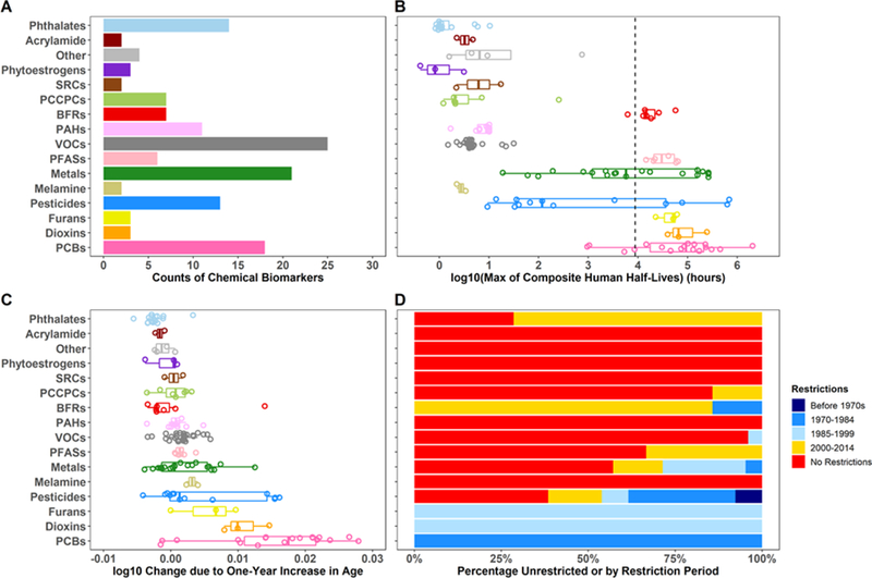
Characteristics of the 141 NHANES chemical biomarkers for 16 classes, including (A) the number of chemical biomarkers for each colored-specific chemical class, (B) ranges of log-transformed composite half-lives in hours, (C) ranges of linear age coefficients $({\beta }_{age}^{linear}{}^{\prime }s)$, defined as the log change in chemical concentration due to a one-year increase in age, and (D) percentage of unrestricted or restricted chemicals per class. Colors of the restriction types only applied to (D) and are also used in Figure 3. BFRs, Brominated Flame Retardants; SRCs, Smoking Related Compounds; PAHs, Polycyclic Aromatic Hydrocarbons; PCCPCs, Personal Care and Consumer Product Compounds; VOCs, Volatile Organic Compounds; PFASs, Per- and Polyfluoroalkyl substances; PCBs, Polychlorinated Biphenyls. Models were adjusted for age centered at $\overline{X_{age}}$ survey cycle, sex, race/ethnicity, poverty income ratio, blood cotinine concentrations, and urinary creatinine concentrations.

Figure 2C shows ranges of ${\beta }_{age}^{linear}{}^{\prime }s$ for each chemical class with numerical values in SI Table S13. These values are interpreted as the log change in chemical concentration for a one-year increase in age. The majority of chemicals from PCBs, Furans, Dioxins, Melamine, Metals, and Pesticides along with a single BFR (2,2',4,4',5,5'-hexabromobiphenyl) have high positive ranges of ${\beta }_{age}^{linear}{}^{\prime }s$, indicating higher concentrations in the older population. In contrast, most of the phthalates, SRCs, and BFRs along with a few VOCs, PCCPCs, PAHs, and phytoestrogens have negative ${\beta }_{age}^{linear}{}^{\prime }s$, reflecting higher concentrations in younger individuals. The majority of chemical biomarkers have ${\beta }_{age}^{linear}{}^{\prime }s$ between −0.01 and 0.01, suggesting small or no differences in chemical biomarker levels across the life-stages.

Figure 2D shows the proportions of unrestricted or restricted chemicals for each class, and SI Table S14 tabulates the restriction dates. Since the latest data were from 2013–2014, chemicals with restriction dates after 2014 are categorized as having no restriction. Chemical classes with higher proportions of unrestricted chemicals include Acrylamide, Other, SRCs, VOCs, and Melamine, and these have limited ${\beta }_{age}^{linear}{}^{\prime }s$ In contrast, PCBs, Dioxins, and Furans show higher proportions of historically restricted chemicals and have the highest ${\beta }_{age}^{linear}{}^{\prime }s$ and high half-lives. The majority of BFRs, PCCPCs, and PFASs have been restricted more recently and have limited ${\beta }_{age}^{linear}{}^{\prime }s$ despite PFASs having high half-lives. The Metal and Pesticides classes demonstrate a wide variety of restriction types, with most of the persistent chemicals in these classes having been restricted before the turn of the century.

SI Figure S1, Text S2, and Table S15 further analyze changes in biomarker levels over the NHANES cycles, demonstrating a decrease in chemical biomarker levels over time for the majority of pesticides and PFASs show, while a few pesticides, phthalates, and PAHs have increasing time trends.

3.3. Influence of Temporal Determinants on Linear Age-Based Trends

To understand the influence of chemical persistence in the body, time trends, and restriction dates on differences in chemical biomarker concentrations across the life-stages, we examined the association between the ${\beta }_{age}^{linear}{}^{\prime }s$ and human whole body elimination half-lives for all chemical biomarkers, color-coded by 1) restriction dates (Figure 3) and by 2) time trend trajectories (Figure S2). Chemical biomarkers with half-lives less than one year have ${\beta }_{age}^{linear}{}^{\prime }s$ ranging from −0.01 to 0.01, indicating limited variation across life-stages. For these chemicals, cross-sectional biomonitoring data is primarily reflective of present exposures in different age groups or populations (Quinn and Wania 2012). In contrast, chemical biomarkers with half-lives greater than one year demonstrate more variation across life-stages and show a positive association between the ${\beta }_{age}^{linear}{}^{\prime }s$ and half-lives. The majority of these persistent chemicals were banned or phased out between the 1970s and 1999 (blue markers in Figure 3). This implies exposures of the younger population have been strongly reduced, and that higher concentrations observed in the older population are likely due to historical exposures and long biological half-lives. Despite the long half-lives of BFRs and PFASs, ${\beta }_{age}^{linear}{}^{\prime }s$ of these chemical classes are substantially lower than those of other persistent substances with similar half-lives. The lower ${\beta }_{age}^{linear}{}^{\prime }s$ with age may be explained by the fact that these chemicals have been recently restricted or are still in use (red and yellow markers in Figure 3) and that current exposures remain higher than exposures to legacy pollutants that were banned earlier. Of special concern are chemicals with negative ${\beta }_{age}^{linear}{}^{\prime }s$ since these chemicals are of higher levels in the younger population compared to the aged population. Most of these chemicals are unrestricted (red markers in Figure 3) and demonstrate an increasing or stable time trend (red and orange markers in Figure S2).

Figure 3.

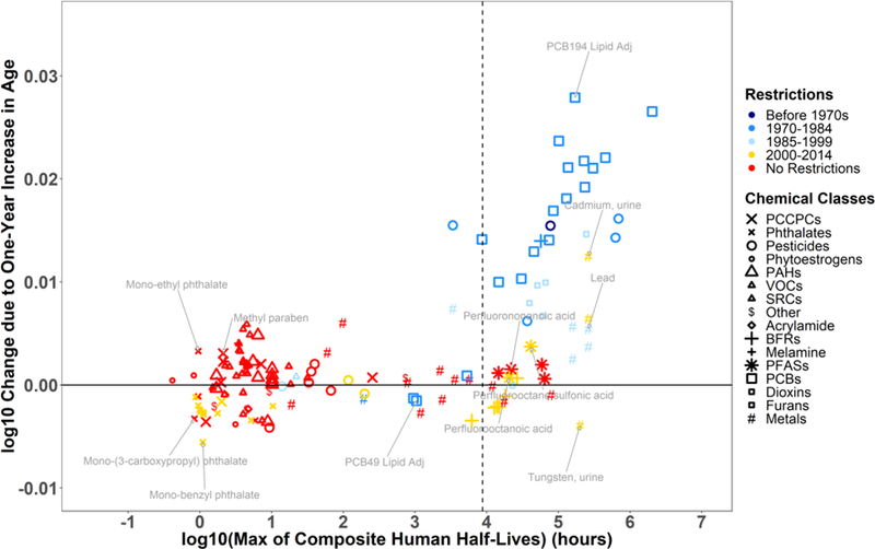
Association between linear age coefficients $({\beta }_{age}^{linear}{}^{\prime }s)$ and chemical persistency in the human body for 141 substances with symbols indicating the different chemical classes. The colors indicate the time period during which the compound was restricted (same as Figure 2D). Models are adjusted for age centered at $\overline{X_{age}}$, survey cycle, sex, race/ethnicity, poverty income ratio, blood cotinine concentrations, and urinary creatinine concentrations. See Figure 2 for abbreviations.

3.4. Nonlinear Age-Based Pattern of Higher Levels in Children

Since a linear relationship between age and log-transformed biomarker levels may not be representative for chemicals that display a nonlinear relationship with age, we refined the chemical-specific regression models to have age squared centered at $X_{age}$ as another main predictor to better characterize this relationship. Figure 4 summarizes the results for age from the quadratic regression model by presenting the association between ${\beta }_{ag{e}^2}$ and ${\beta }_{age}$ for all chemical biomarkers. The chemical classes are indicated by difference shapes, while the colors show the different categories of fold difference in chemical biomarker levels between a child of 5 years and adult of 31.88 years. For instance, mono-benzyl phthalate levels in 5-years-old children are on average 2.598 times higher compared to those for 31.88-years-old adults. A positive ${\beta }_{ag{e}^2}$ indicates a convex (or u-shaped) relationship between log-transformed chemical biomarker levels and age, while a negative ${\beta }_{ag{e}^2}$ indicates a concave or (n-shaped) relationship.

Figure 4.

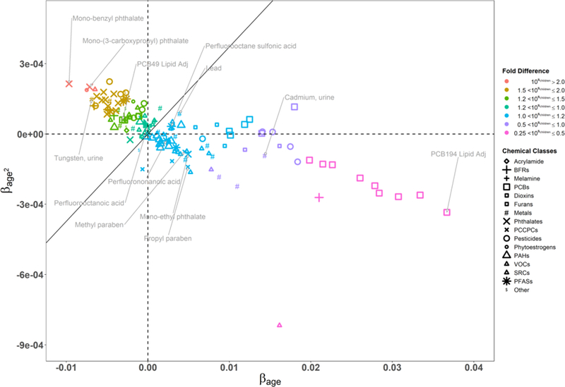
Association between ${\beta }_{ag{e}^2}$ and ${\beta }_{age}$ for 141 substances with symbols indicating chemical classes and colors indicating categories of fold difference in biomarker levels between a child of 5 years and adult of 31.88 years. The boundary line ${\beta }_{ag{e}^2}/{\beta }_{age}>1/26.9$ differentiates chemicals of higher levels in children from those of higher levels in the older population. Models were adjusted for age centered at $\overline{X_{age}}$, age centered at $\overline{X_{age}}$ squared, survey cycle, sex, race/ethnicity, poverty income ratio, blood cotinine concentrations, and urinary creatinine concentrations. See Figure 2 for abbreviations.

Chemicals in the upper left quadrant are of interest, since these are higher in 5-years-old children compared to 31.88-years-old adults by more than a factor of 2. Most of these chemicals are metals, pesticides, and phthalates used in building materials and articles. Based on Equation 2, the boundary line corresponds to equal biomarker levels for a child of 5 years and an adult of 31.88 years. Chemicals above and to the left of the boundary line $({\beta }_{ag{e}^2}/{\beta }_{age}>\frac{1}{\overline{X_{age}}-X_{age}}=\frac{1}{26.9})$ have a downward and convex trend across age groups, implying the highest biomarker levels for the youngest participants. The highest levels in children compared to adults of average age are observed for mono-benzyl phthalate, O-Desmethylangolensin (O-DMA), mono-(3-carboxypropyl) phthalate, 2-amnothiazolne-4-carbxylic acid and tungsten. SI Table S7 provides a detailed list of chemicals ranked from highest to lowest relative value between children and adults of average age.

To further compare chemical biomarker distributions across the different life-stages and identify linear and nonlinear age-based trends, we stratified these distributions into 11 age groups (Figure 5) and selected example chemicals to represent the specific age-group trends within a chemical class. The geometric mean of the measured chemical biomarker levels for each age group is represented by a gray circle, while the geometric mean of the predicted chemical biomarker levels is indicated by a brown triangle. Outliers are represented by dash marks outside of the distributions of chemical biomarker concentration. A residual standard error (RSE) of 0 implies the model perfectly predicts the log-transformed biomarker levels. Geometric mean of predicted chemical biomarker levels for the 1–2 age group is unavailable, since cotinine was not measured in these participants.

Overall, the nonlinear regression models predicted the measured geometric means fairly well, particularly for children, middle-aged adults, and the elderly. The models, however, overestimated biomarker levels for tungsten, phthalates, and parabens in the adolescent age group, and underestimated lead in the toddler age group, indicating the need for a higher order polynomial model rather than a parabolic regression model for these specific cases.

The following section analyzes in further detail these age trends by chemical class and type of usage.

3.5. Age-Based Trends by Chemical Class

3.5.1. PCBs, Dioxins, and Furans

For PCBs, there are three main age patterns: a slight downward and convex trend, a steep upward and concave trend, and no trend across the life stage (Figure 4). The PCBs with half-lives less than one year (Figure 3) showed little or no variation in chemical biomarker concentrations by age. PCB 49 (Figure 5A) and PCB 44 are the only two PCBs for which the youngest participants have the highest biomarker levels, with their negative ${\beta }_{age}$ and positive ${\beta }_{ag{e}^2}$ characterizing a slight downward and convex trend across the age groups. This might indicate children are exposed through a pathway specific to these two congeners. In contrast, the more persistent PCBs, dioxins and furans have higher concentrations in the older population, except for 1,2,3,4,6,7,8-Heptachlorodibenzofuran (half-life of 3.58 years), which has a ${\beta }_{age}$ of −0.0021. This may indicate ongoing exposure despite this chemical having been banned much earlier. With the highest ${\beta }_{age}$ of 0.037 and a ${\beta }_{ag{e}^2}$ of −0.00033, PCB 194 illustrated well (Figure 5B) a steep upward and concave trend across the age groups with the oldest participants having at most a 100-fold difference in biomarker levels compared to the youngest age group. This tendency is confirmed in the pooled serum concentrations observed for four age groups (12–19, 20–39, 40–59, 60+) in 2005–2008 by different race-sex combinations (details in Text S3, Section 4). Age is a good predictor of biomarker levels for the more persistent PCBs, with an adjusted correlation coefficient (R²) ranging between 0.37 and 0.72 for most PCBs, with the exception of PCB 28 (R² = 0.035), PCB 44 (R² = 0.036), and PCB 49 (R² = 0.041).

3.5.2. PFASs

PFASs are also highly persistent, but their ${\beta }_{age}{}^{\prime }s$ do not vary as substantially as those of PCBs. Most of the PFASs have ${\beta }_{age}{}^{\prime }s$ close to 0, indicating there is little to no difference by age and implying ongoing exposures. PFNA shows little to no variation across age groups (Figure 5C). On the other hand, PFOA and PFOS show a slight upward and convex trend across the age groups (Figure S5 and 5D). This is confirmed by a ${\beta }_{age}$ of 0.0029 and a ${\beta }_{ag{e}^2}$ of 3.27E-05 for PFOS, and by a ${\beta }_{age}$ of −5.80E-05 and a ${\beta }_{ag{e}^2}$ of 2.97E-05 for PFOA. Since PFOS and PFOA were phased out in 2002 (3M Company 2000; US EPA 2003, 2007), differences across the age groups are substantially smaller than those observed in PCB 194, which was banned in 1979. Such differences across the life-course, however, are expected to increase in the future as articles and materials containing PFASs will reach the end of their usable life. A specific trend analysis is presented in the next section for these PFASs to illustrate how the age-based trends vary across the different cycles.

3.5.3. Metals

Another class of highly persistent chemicals is the Metals. Although many of the metals demonstrate a stable trajectory over time (yellow markers in Figure S2), there are high variations in chemical biomarker levels across the life-stages, with three different types of age group patterns evident (Figure 3 and 4). Cadmium demonstrates higher urinary concentrations in the older population with a ${\beta }_{age}$ of 0.014 and a ${\beta }_{ag{e}^2}$ of −9.22E-05, denoting a slight upward and concave trend across the age groups (Figure S6). Lead is one of the few chemicals with measurements in children 1 to 4 years old. Although the ${\beta }_{age}$ of lead (0.0039) is not as high as that of cadmium, the convex trend of lead $({\beta }_{ag{e}^2}=8.72\text{E-05})$ across the age groups indicates the youngest and oldest age groups have the highest biomarker concentrations compared to the other age groups (Figure 5F). Although tungsten has similar persistency to cadmium and lead, it has a ${\beta }_{age}$ of −0.0069 and a ${\beta }_{ag{e}^2}$ of 0.00015, indicating a downward, convex trend across the age groups (Figure 5E). This is also indicative of high and ongoing exposures in the younger population.

3.5.4. Phthalate and Parabens

Most phthalates are used as plasticizers. These phthalates show a similar age group pattern to that of mono-(3-carboxypropyl) phthalate - a metabolite of mono-n-butyl phthalate, di-n-butyl phthalate, mono-n-octyl phthalate, and di-n-octyl phthalate (Figure 5G), and mono-benzyl phthalate (Figure 5H), with the highest concentration apparent in the youngest age group, a decrease during adolescence and young adulthood, and then stabilization for older age groups. In contrast, mono-ethyl phthalate is mostly used in cosmetics and demonstrates a very different age group pattern from those in its chemical family (Figure 5I). It has a similar age group pattern to chemicals used in cosmetics such as methyl paraben (Figure 5J). Methyl paraben has a slight upward and concave trend across the 5–12, to 13–18, and 19–28 years-old participants. Its levels peak for the mature adults and show a slight decrease in older age groups.

3.6. Change in Age-Based Trends of PFASs over Time

To determine how the age-based trends are changing over time, we fitted smooth curves to the life-stage changes in chemical biomarker concentration for each available NHANES cycles and conducted a series of linear regression models stratified by cycle to extract the ${\beta }_{age,k}$’s The ${\beta }_{age,k}$’s shows the overall difference in chemical biomarker concentration between the young and aged populations for a given NHANES kth cycle. Understanding how these ${\beta }_{age,k}$’s change over time provides insight on how the difference between the youth and elderly changes across the cycles. In addition, these ${\beta }_{age,k}$’s will help determine how long a time lapse must occur between the restriction date and sample collection date in order to observe these life-stage differences.

PFASs were further analyzed, since some have been recently phased out and have measurements spanning over six or more cycles. PFOS, Perfluorohexane sulfonic acid (PFHxS), PFOA, Perfluorodecanoic acid (PFDA), PFNA, and 2-(N-methyl-PFOSA) acetate were selected due to their high detection frequencies for each available cycle. Figure 6 presents how the age-based trends are changing over time. Each curve represents the variation in chemical biomarker concentration by age for a given NHANES cycle. A vertical shift in an ith cycle curve indicates how the chemical biomarker concentrations have increased or decreased compared to those in the (i-1)th cycle. The steepness of the curve shows the rate at which the log-transformed chemical concentration is changing with each one-year increase in age for a given cycle, providing insight on how the differences in chemical biomarker levels between the youth and elderly are changing over time. An increase in the ${\beta }_{age,k}$’s indicates the difference between the young and aged populations are expanding over time.

Figure 6.

Chemical biomarker concentrations across the life-stages stratified by NHANES cycles for (A) PFOS, (B) PFHxS, (C) PFOA, (D) PFDA, (E) PFNA, and (F) 2-(N-methyl-PFOSA) acetate. (G) 95% confidence intervals for the cycle-specific age coefficients for PFOS, PFHxS, PFOA, PFDA, PFNA, and 2-(N-methyl-PFOSA) acetate. The cycle-specific age coefficients (${\beta }_{age,k}$ ‘s) with age shows the adjusted rate at which the chemical concentration is changing for a one-year increase in age for a particular cycle. Models were adjusted for age, sex, race/ethnicity, poverty income ratio, blood cotinine concentrations, and urinary creatinine concentrations.

Between 1999–2000, the ${\beta }_{age,1}$ for PFOS is 6.51E-4 (p-value = 0.025). If we assume chemical biomarker concentrations change linearly with age, then this value implies a 1.13-fold difference (10^80×6.51E-4 = 1.13) in chemical concentration between an 80-year old participant and a newborn (aged 0). Between 2013–2014, the ${\beta }_{age,8}$ is 6.49E-3 (p-value = 2.63E-59) with a 3.3 fold difference. This suggests that a decade after the phase-out of PFOS, the aged population has approximately a 3-fold difference in PFOS levels compared to the youth (Figure 6A and 6G). As the biomarker levels of PFOS and 2-(N-methyl-PFOSA) acetate decrease across the cycles, illustrated by the downward shifts in the concentration-age curves, the difference between the youth and elderly increases. This is evidenced by the increasing steepness of these curves (Figure 6A and 6F) and the upward trend in ${\beta }_{age,k}$’s (Figure 6G). These patterns imply the use of PFOSA stopped around the time of the restrictions on PFOS and PFOA in 2002 (US EPA 2003, 2007). A similar pattern can be observed with PFHxS and PFOA concentrations, but the differences between the young and aged populations for these chemicals do not change as drastically they do for PFOS and PFOSA (Figure 6B, 6C, and 6G). These patterns suggest that as the time increases between the restriction and sample collection dates, the differences by age will become more prominent.

On the other hand, PFHxS, PFDA, and PFNA display different trends over time. For instance, biomarker levels for PFHxS initially decrease during 1999–2006, increase in 2007–2008, and then decrease again for the more recent NHANES cycles. For PFDA, biomarker levels increase from 1999 to 2006 and then decrease afterward. Biomarker levels of PFNA increase during the early NHANES cycles and then decrease after 2009–2010, but the PFNA levels for 2013–2014 are on average higher than those between 1999–2000 especially for children. The cycle-specific age coefficients for PFNA fluctuate during the early NHANES cycles but then show a strictly increasing trend after 2007–2008 (Figure 6E and 6G). These fluctuations in biomarker levels suggest PFHxS, PFDA, and PFNA may have been used as substitutes for PFOS and PFOA and reflect ongoing exposure throughout the population.

4. DISCUSSION

In this article, we present a comprehensive analysis of age-based and time trends in chemical biomarker concentrations in the US population. We have accounted for biological half-lives of chemicals, type of usage, and historical events, i.e., dates of chemical bans and phase-outs, which are expected to influence population-level exposures. These results provide insight on population exposure trajectories. They are also informative for differentiating legacy exposures from current exposures and for identifying chemicals of higher levels in the younger population.

For restricted chemicals, our data confirm that a minimum persistence of 1 year in the human body is necessary to observe substantial differences between the young population and historically exposed adults. Biological half-life is not the only determinant of high chemical biomarker levels in the aged population, however. Studies on age-based and time trends of biomonitoring data have suggested the potential influences of bans, phase-outs, bioaccumulation, metabolic rates, and consumer product usage on such trends (Calafat et al. 2007; Kato et al. 2011; Sjödin et al. 2008; Xue et al. 2014; Zota et al. 2014), with the most influential determinant for simulated longitudinal data being the time lapse between the peak of emission and the sample collection (Quinn and Wania 2012). Thus, elevated concentrations in the elderly population are primarily due to a combination of past exposure and slow elimination. Using measured biomonitoring data for a wide range of chemicals, we confirm that chemicals with high age coefficients primarily have a biological half-life longer than 1 year and have been banned or phased out for longer than the chemical’s half-life (Quinn and Wania 2012). This evidences the efficacy of public health interventions, such as the International Stockholm Convention on Persistent Organic Pollutant, to reduce or prevent high exposures and associated health outcomes for the younger population (Prüss-Ustün et al. 2011; WHO 2016).

PFASs are also persistent, with half-lives ranging from 1.6 years to 7.3 years, yet show minimal differences in biomarker concentrations across the life-stages. These substances demonstrate contrasting age-based patterns even within the same family. For instance, we observed a substantial reduction in PFOA and PFOS levels in children, but levels of PFNA and PFHxS in children during 2013–2014 are still higher or equal than those in the earlier NHANES cycles. This indicates ongoing and higher exposures for the younger population. Such exposures to PFASs may occur through breastfeeding (Kärrman et al. 2007; Mogensen et al. 2015; Thomsen et al. 2010) or drinking contaminated water (Gyllenhammar et al. 2018; Mondal et al. 2012). In addition, this pattern could be due to the fact that some of these chemicals were recently phased-out, or due to the short time lapse between the emission peak and the sample collection. The time lapse of a decade for PFASs is shorter than the time lapse of almost 30 years for PCBs. Thus, it can be inferred that as this time lapse increases, especially if it exceeds the half-life of the substance, the difference in PFASs concentrations by age will continue to increase (Quinn and Wania 2012, Gomis et al. 2017).

While cadmium levels are lower in the younger population, this is not the case for lead and especially tungsten for which the younger population has surprisingly higher biomarker levels. Higher lead levels have been attributed to consumer products usage, such as toys and children jewelry (Guney and Zagury 2013; Kumar and Pastore 2007), exposures to dust and soil (Dixon et al. 2009; Lanphear et al. 1998), and exposures via maternal transfer in utero or during breastfeeding (Bhattacharyya 1983; Silbergeld 1991). For the older participants, high lead levels may be due to leaded gasoline combustion before tetraethyl lead in gasoline was banned (Newell and Rogers 2003). High tungsten levels in children may be due to exposures to contaminated soil, articles from parents’ workspace, and electrical devices (ATSDR 2005; Kampmann et al. 2002). The overall trend of higher levels in the 5–12 years old followed by a downward, convex trend across the older age groups suggests exposures in children may be driven by factors specific to this susceptible population. Hence, further research is necessary to elucidate potential reasons for higher exposures in children.

For several less-persistent chemicals, such as phthalates that are widely used in consumer products, younger individuals seem to have been highly exposed, in addition to some persistent chemicals such as the BFRs, PFASs and lead. Our results suggest age-based trends in biomarker levels reflect product usage trends. Most phthalates show a plasticizer age pattern with higher concentrations in the 5–12 years old age group followed by a downward, convex trend across older age groups, which is quantified by a positive ${\beta }_{ag{e}^2}$ and negative ${\beta }_{age}$. Children may be highly exposed to these chemicals through frequent contact with flooring materials (Healthy Building Network 2017; Just et al. 2015; Xu et al. 2010) and toys (Hileman 2007), which are products that typically have high levels of plasticizers. Also, children may more readily absorb these compounds (Royce and Needleman 1992). Metabolic rate is known to vary across age with a peak occurring during childhood and then stabilizing or decreasing during the senior years (Shimokata and Kuzuya 1993; Speakman 2005). In contrast, mono-ethyl phthalate is used in personal care products (Api 2001) and shows a different concave pattern similar to other personal care products such as parabens and triclosan. The increase in exposure from children to teenagers may be explained by a greater use of cosmetic and/or skin care products during the teenage years (Calafat et al. 2010; Freedman 1984; Gentina et al. 2012). Comparing chemical levels by age group and quantifying trends across the age groups with ${\beta }_{ag{e}^2}$ and ${\beta }_{age}$ enables us to identify two interesting clusters: 1) a cluster of phthalates used as plasticizers and 2) a cluster of chemicals used in personal care products. Mono-ethyl phthalate was shown to cluster with PCCPCs instead of with those in its chemical family. These age-based clusters of chemicals with similar product usage suggest a possibility to develop product-specific archetypes of intake pattern with e.g. a concave age curve for personal care products versus a convex age curve for plasticizers in articles and building materials. These archetypes could then be used to help extend mechanistic modelling approaches to predict direct exposures to chemicals used in consumer products.

The present study has a number of limitations. By comparing chemical biomarker levels by age group, we have identified several chemicals, such as lead, tungsten, and phthalates, to be of higher concentrations in the younger population than in the older population. Although we have identified a number of potential reasons for higher exposures in children, we have not accounted for differences in metabolic rate within our models. Future extensions could determine surrogate variables to develop a scoring system to quantitatively represent metabolic rate and understand how it could confound age and chemical biomarker concentrations. Finally, while we demonstrated an overarching, statistical approach to identify chemicals that are of higher concentrations in children, there is a need to understand toxicological effects of these chemicals along with identifying sources and pathways of exposures to prevent elevated chemical levels and the onset of adverse health effects (Prüss-Ustün et al. 2011; WHO 2016; Zota et al. 2017).

Though we defined an age pattern of concern for children, quantifying exposure for young children, especially those below the age of 4, was limited to a few chemical biomarkers such as lead, manganese, cadmium, methyl mercury, cotinine, acrylamide, and glycideamide. As shown with lead, predictions were unavailable for children below the age of 2, since cotinine was not measured for these participants. Thus when more measurements for children become available, future extensions could incorporate such data to better quantify and predict exposure for this susceptible population.

Geographical location has been identified as a confounder of chemical exposure disparities, particularly for heavy metals (Hough et al. 2004; Voutsa and Samara 2002), but we did not consider this as a covariate in this study. Future studies could consider geospatial variations in chemical biomarker concentrations to systematically address geographical location as a confounder.

For lipophilic chemicals, we preferred the lipid-adjusted measurements, since these measurements were normalized to the blood lipid content of the participants. In addition, adipose content tends to increase as a person age, which can potentially lead to higher concentrations of more lipophilic compounds in the aged population. Even though BMI could modulate the concentration-age associations, we did not consider it as a covariate, since we wanted to study the BMI mediated effect of age on chemical biomarker levels. Future extensions could further explore the confounding nature of BMI on age-based and time trends of chemical biomarker levels.

5. CONCLUSIONS

This study presents a framework for systematically analyzing and interpreting biomonitoring data, to better understand chemical biomarker differences across the life-stages. We suggest different criteria for determining which chemicals are reflective of legacy exposures vs. current exposures and identify an age pattern of concern when longitudinal data are unavailable or incomplete. We confirm the criteria indicative of legacy exposure as follows: 1) biological half-life of at least one year, 2) decreasing average biomarker concentration over time due to the chemical being banned or phased out, and 3) the time lapse between emission peak and the sample collection exceeding the human elimination half-life. For chemicals below the one-year half-life mark, cross-sectional biomonitoring data mostly reflect recent intake rates. In addition to confirming the criteria for legacy versus relevant exposures, the complementary analysis combining a series of regression models with systemized stratified analyses by age group helped us define an age-based pattern for identifying chemicals of higher and ongoing exposures in children. This is especially evident when a chemical biomarker has an increasing or stable time trajectory, demonstrates a convex relationship with age, and is of higher concentration in the younger population. The presented framework can be used to help facilitate risk stratification and guide targeted interventions.

Highlights.

• We characterized linear and nonlinear age-based trends for 141 chemical biomarkers

• Minimum 1 year persistence in humans to have adults with historically high exposure

• We defined a metric to identify chemicals of high and ongoing exposure in children

• Several phthalates, pesticides, and metals reflect ongoing exposure in children

• Determined temporal changes in age trends for 6 Per- and Polyfluoroalkyl Substances

References

- 3M Company. 2000. Voluntary use and exposure information profile for perfluorooctanoic acid and salts. USEPA Administrative Record AR226–0595.
- Arnot JA, Brown TN, Wania F. 2014. Estimating screening-level organic chemical half-lives in humans. Environmental Science & Technology 48:723–730. [DOI] [PubMed] [Google Scholar]
- ATSDR. 2005. Toxicological profile for tungsten Available: https://www.atsdr.cdc.gov/toxprofiles/tp186.pdf. [PubMed]
- Barr DB, Wilder LC, Caudill SP, Gonzalez AJ, Needham LL, Pirkle JL. 2005. Urinary creatinine concentrations in the u.S. Population: Implications for urinary biologic monitoring measurements. Environmental health perspectives 113:192–200. [DOI] [PMC free article] [PubMed] [Google Scholar]
- Benjamini Y, Hochberg Y. 1995. Controlling the false discovery rate: A practical and powerful approach to multiple testing. Journal of the Royal Statistical Society Statistical Methodology Series B 57:289–300. [Google Scholar]
- Benowitz NL. 1999. Biomarkers of environmental tobacco smoke exposure. Environmental Health Perspectives 107:349–355. [DOI] [PMC free article] [PubMed] [Google Scholar]
- Bhattacharyya MH. 1983. Bioavailability of orally administered cadmium and lead to the mother, fetus, and neonate during pregnancy and lactation: An overview. Science of The Total Environment 28:327–342. [DOI] [PubMed] [Google Scholar]
- Bornschein RL, Succop PA, Krafft KM, Clark CS, Peace B, Hammond PB. 1986. Exterior surface dust lead, interior house dust lead and childhood lead exposure in an urban environment United States. [Google Scholar]
- Calafat AM, Wong L-Y, Kuklenyik Z, Reidy JA, Needham LL. 2007. Polyfluoroalkyl chemicals in the u.S. Population: Data from the national health and nutrition examination survey (nhanes) 2003–2004 and comparisons with nhanes 1999–2000. Environmental Health Perspectives 115:1596–1602. [DOI] [PMC free article] [PubMed] [Google Scholar]
- Calafat AM, Ye X, Wong L-Y, Bishop AM, Needham LL. 2010. Urinary concentrations of four parabens in the us population: Nhanes 2005–2006. Environmental Health Perspectives 118:679–685. [DOI] [PMC free article] [PubMed] [Google Scholar]
- CDC. 2009. Fourth national report on human exposure to environmental chemicals Available: https://www.cdc.gov/exposurereport/pdf/fourthreport.pdf. [PubMed]
- Dixon SL, Gaitens JM, Jacobs DE, Strauss W, Nagaraja J, Pivetz T, et al. 2009. Exposure of u.S. Children to residential dust lead, 1999–2004: Ii. The contribution of lead-contaminated dust to children’s blood lead levels. Environ Health Perspect 117:468–474. [DOI] [PMC free article] [PubMed] [Google Scholar]
- FDA. 2018. Limiting lead in lipstick and other cosmetics Available: https://www.fda.gov/Cosmetics/ProductsIngredients/Products/ucm137224.htm#initial_survey.
- Fowler T. A brief history of lead regulation. Science Progress where science, technology, and policy meet. 2008.
- Freedman RJ. 1984. Reflections on beauty as it relates to health in adolescent females. Women & Health 9:29–45. [DOI] [PubMed] [Google Scholar]
- Gentina E, Palan KM, Fosse-Gomez M-H. 2012. The practice of using makeup: A consumption ritual of adolescent girls. Journal of Consumer Behaviour 11:115–123. [Google Scholar]
- Gomis MI, Vestergren R, MacLeod M, Mueller JF, Cousins IT. 2017. Historical human exposure to perfluoroalkyl acids in the united states and australia reconstructed from biomonitoring data using population-based pharmacokinetic modelling. Environ Int 108:92–102. [DOI] [PubMed] [Google Scholar]
- Guney M, Zagury GJ. 2013. Contamination by ten harmful elements in toys and children’s jewelry bought on the north american market. Environmental Science & Technology 47:5921–5930. [DOI] [PubMed] [Google Scholar]
- Gyllenhammar I, Benskin JP, Sandblom O, Berger U, Ahrens L, Lignell S, et al. 2018. Perfluoroalkyl acids (pfaas) in serum from 2–4-month-old infants: Influence of maternal serum concentration, gestational age, breast-feeding, and contaminated drinking water. Environ Sci Technol 52:7101–7110. [DOI] [PubMed] [Google Scholar]
- Healthy Building Network. 2017. Pharos project
- Hileman B 2007. California bans phthalates in toys for children. Chemical & Engineering News 85:12. [Google Scholar]
- Hornung RW, Reed LD. 1990. Estimation of average concentration in the presence of nondetectable values. Applied Occupational and Environmental Hygiene 5:46–51. [Google Scholar]
- Hough RL, Breward N, Young SD, Crout NMJ, Tye AM, Moir AM, et al. 2004. Assessing potential risk of heavy metal exposure from consumption of home-produced vegetables by urban populations. Environmental Health Perspectives 112:215–221. [DOI] [PMC free article] [PubMed] [Google Scholar]
- Jl P, Dj B, Ew G, al e. 1994. The decline in blood lead levels in the united states: The national health and nutrition examination surveys (nhanes). JAMA 272:284–291. [PubMed] [Google Scholar]
- Jolliet O, Wenger Y, Adriaens P, Chang CW, Chen Q, Franzblau A, et al. Influence of age on serum dioxin concentratins as a function of cogender half-life and historical peak food contamination. In: Proceedings of the Dioxin 2008 Conference, 2008. Birmingham, England. [Google Scholar]
- Just AC, Miller RL, Perzanowski MS, Rundle AG, Chen Q, Jung KH, et al. 2015. Vinyl flooring in the home is associated with children’s airborne butylbenzyl phthalate and urinary metabolite concentrations. Journal of Exposure Science & Environmental Epidemiology 25:574–579. [DOI] [PMC free article] [PubMed] [Google Scholar]
- Kampmann C, Brzezinska R, Abidini M, Wenzel A, Wippermann C-F, Habermehl P, et al. 2002. Biodegradation of tungsten embolisation coils used in children. Pediatric Radiology 32:839–843. [DOI] [PubMed] [Google Scholar]
- Kärrman A, Ericson I, van Bavel B, Darnerud PO, Aune M, Glynn A, et al. 2007. Exposure of perfluorinated chemicals through lactation: Levels of matched human milk and serum and a temporal trend, 1996–2004, in sweden. Environmental Health Perspectives 115:226–230. [DOI] [PMC free article] [PubMed] [Google Scholar]
- Kato K, Wong L-Y, Jia LT, Kuklenyik Z, Calafat AM. 2011. Trends in exposure to polyfluoroalkyl chemicals in the u.S. Population: 1999−2008. Environmental Science & Technology 45:8037–8045. [DOI] [PubMed] [Google Scholar]
- Korn EL, Graubard BI. 1991. Epidemiologic studies utilizing surveys: Accounting for the sampling design. American Journal of Public Health 81:1166–1173. [DOI] [PMC free article] [PubMed] [Google Scholar]
- Kumar A, Pastore P. 2007. Lead and cadmium in soft plastic toys. Current Science 93:818–822. [Google Scholar]
- Lanphear BP, Matte TD, Rogers J, Clickner RP, Dietz B, Bornschein RL, et al. 1998. The contribution of lead-contaminated house dust and residential soil to children’s blood lead levels. A pooled analysis of 12 epidemiologic studies. Environ Res 79:51–68. [DOI] [PubMed] [Google Scholar]
- Levallois P, St-Laurent J, Gauvin D, Courteau M, Prévost M, Campagna C, et al. 2014. The impact of drinking water, indoor dust and paint on blood lead levels of children aged 1–5 years in montréal (québec, canada). Journal of Exposure Science & Environmental Epidemiology 24:185–191. [DOI] [PMC free article] [PubMed] [Google Scholar]
- Mathee A, Röllin H, Levin J, Naik I. 2007. Lead in paint: Three decades later and still a hazard for african children? Environmental Health Perspectives 115:321–322. [DOI] [PMC free article] [PubMed] [Google Scholar]
- Mogensen UB, Grandjean P, Nielsen F, Weihe P, Budtz-Jorgensen E. 2015. Breastfeeding as an exposure pathway for perfluorinated alkylates. Environ Sci Technol 49:10466–10473. [DOI] [PMC free article] [PubMed] [Google Scholar]
- Mondal D, Lopez-Espinosa M-J, Armstrong B, Stein CR, Fletcher T. 2012. Relationships of perfluorooctanoate and perfluorooctane sulfonate serum concentrations between mother–child pairs in a population with perfluorooctanoate exposure from drinking water. Environmental Health Perspectives 120:752–757. [DOI] [PMC free article] [PubMed] [Google Scholar]
- NCHS. 2005a. Metals - urine (l06hm_b) Available: https://wwwn.cdc.gov/Nchs/Nhanes/2001-2002/L06HM_B.htm.
- NCHS. 2005b. Metals - urine (lab06hm) Available: https://wwwn.cdc.gov/Nchs/Nhanes/1999-2000/LAB06HM.htm.
- NCHS. 2010. Continuous nhanes web tutorial sample design
- Newell R, Rogers K. 2003. The u.S. Experience with the phasedown of lead in gasoline. Resources for the Future
- OECD. 2004. The report from the expert group on (quantitative) structure-activity relationships [(q) sars] on the principles for the validation of (q) sars
- OECD. 2014. Guidance document on the validation of (quantitative) structure-activity relationship [(q)sar] models
- Prüss-Ustün A, Vickers C, Haefliger P, Bertollini R. 2011. Knowns and unknowns on burden of disease due to chemicals: A systematic review. Environmental Health 10:9. [DOI] [PMC free article] [PubMed] [Google Scholar]
- Quinn CL, Wania F. 2012. Understanding differences in the body burden–age relationships of bioaccumulating contaminants based on population cross sections versus individuals. Environmental Health Perspectives 120:554–559. [DOI] [PMC free article] [PubMed] [Google Scholar]
- Richter AP, Bishop EE, Wang J, Swahn HM. 2009. Tobacco smoke exposure and levels of urinary metals in the u.S. Youth and adult population: The national health and nutrition examination survey (nhanes) 1999–2004. International Journal of Environmental Research and Public Health 6. [DOI] [PMC free article] [PubMed] [Google Scholar]
- Ritter R, Scheringer M, MacLeod M, Moeckel C, Jones KC, Hungerbühler K. 2011. Intrinsic human elimination half-lives of polychlorinated biphenyls derived from the temporal evolution of cross-sectional biomonitoring data from the united kingdom. Environmental Health Perspectives 119:225–231. [DOI] [PMC free article] [PubMed] [Google Scholar]
- Royce S, Needleman H. 1992. Case studies in environmental medicine: Lead toxicity Atlanta: Agency for Toxic Substances and Disease Registry. [Google Scholar]
- Royston P 1992. Lowess smoothing. Stata Technical Bulletin 1. [Google Scholar]
- Schecter A, Colacino J, Haffner D, Patel K, Opel M, Päpke O, et al. 2010. Perfluorinated compounds, polychlorinated biphenyls, and organochlorine pesticide contamination in composite food samples from dallas, texas, USA. Environmental Health Perspectives 118:796–802. [DOI] [PMC free article] [PubMed] [Google Scholar]
- Services UDoHaH. 2012. Principles of pediatric environmental health why are children often especially susceptible to the adverse effects of environmental toxicants? Available: https://www.atsdr.cdc.gov/csem/ped_env_health/docs/ped_env_health.pdf.
- Shimokata H, Kuzuya F. 1993. Aging, basal metabolic rate, and nutrition. Nihon Ronen Igakkai zasshi Japanese Journal of Geriatrics 30:572–576. [DOI] [PubMed] [Google Scholar]
- Silbergeld EK. 1991. Lead in bone: Implications for toxicology during pregnancy and lactation. Environmental Health Perspectives 91:63–70. [DOI] [PMC free article] [PubMed] [Google Scholar]
- Silva MJ, Barr DB, Reidy JA, Malek NA, Hodge CC, Caudill SP, et al. 2004. Urinary levels of seven phthalate metabolites in the u.S. Population from the national health and nutrition examination survey (nhanes) 1999–2000. Environmental Health Perspectives 112:331–338. [DOI] [PMC free article] [PubMed] [Google Scholar]
- Speakman JR. 2005. Body size, energy metabolism and lifespan. The Journal of Experimental Biology 208:1717–1730. [DOI] [PubMed] [Google Scholar]
- Stevens RG, Jones DY, Micozzi MS, Taylor PR. 1988. Body iron stores and the risk of cancer. New England Journal of Medicine 319:1047–1052. [DOI] [PubMed] [Google Scholar]
- Thomsen C, Haug LS, Stigum H, Froshaug M, Broadwell SL, Becher G. 2010. Changes in concentrations of perfluorinated compounds, polybrominated diphenyl ethers, and polychlorinated biphenyls in norwegian breast-milk during twelve months of lactation. Environ Sci Technol 44:9550–9556. [DOI] [PubMed] [Google Scholar]
- Trudel D, Horowitz L, Wormuth M, Scheringer M, Cousins IT, Hungerbühler K. 2008. Estimating consumer exposure to pfos and pfoa. Risk Analysis: An International Journal 28:251–269. [DOI] [PubMed] [Google Scholar]
- Tsou M-C, Özkaynak H, Beamer P, Dang W, Hsi H-C, Jiang C-B, et al. 2015. Mouthing activity data for children aged 7 to 35 months old in taiwan. Journal of Exposure Science & Environmental Epidemiology 25:388–398. [DOI] [PMC free article] [PubMed] [Google Scholar]
- US Census Bureau. 2014. Age and sex composition in the united states: 2014 Available: https://www.census.gov/data/tables/2014/demo/age-and-sex/2014-age-sex-composition.html.
- US Census Bureau. 2016. Quickfacts united states Available: https://www.census.gov/quickfacts/fact/table/US/PST045217.
- US EPA. 2003. Perfluoroalkyl sulfonates; significant new use rule
- US EPA. 2007. Standards of performance for new stationary sources and emission guidelines for existing sources, municipal waste combustors [PubMed]
- US EPA. 2011. Basic questions and answers for the drinking water strategy contaminant groups effort
- US EPA. 2017. Drinking water contaminants – standards and regulations Available: https://www.epa.gov/dwstandardsregulations/use-lead-free-pipes-fittings-fixtures-solder-and-flux-drinking-water.
- Voutsa D, Samara C. 2002. Labile and bioaccessible fractions of heavy metals in the airborne particulate matter from urban and industrial areas. Atmospheric Environment 36:3583–3590. [Google Scholar]
- WHO. 2016. Public health impact of chemicals: Knowns and unknowns
- Wong F, MacLeod M, Mueller JF, Cousins IT. 2014. Enhanced elimination of perfluorooctane sulfonic acid by menstruating women: Evidence from population-based pharmacokinetic modeling. Environmental Science & Technology 48:8807–8814. [DOI] [PubMed] [Google Scholar]
- Xu Y, Cohen Hubal EA, Little JC. 2010. Predicting residential exposure to phthalate plasticizer emitted from vinyl flooring: Sensitivity, uncertainty, and implications for biomonitoring. Environmental Health Perspectives 118:253–258. [DOI] [PMC free article] [PubMed] [Google Scholar]
- Xue J, Liu SV, Zartarian VG, Geller AM, Schultz BD. 2014. Analysis of nhanes measured blood pcbs in the general us population and application of sheds model to identify key exposure factors. J Expos Sci Environ Epidemiol 24:615–621. [DOI] [PubMed] [Google Scholar]
- Zota AR, Calafat AM, Woodruff TJ. 2014. Temporal trends in phthalate exposures: Findings from the national health and nutrition examination survey, 2001–2010. Environmental Health Perspectives 122:235–241. [DOI] [PMC free article] [PubMed] [Google Scholar]
Associated Data
This section collects any data citations, data availability statements, or supplementary materials included in this article.