Brain and lesion segmentation in multiple sclerosis using fully-convolutional neural networks: A large-scale study

Abstract

Objective:

To investigate the performance of deep learning (DL) based on fully convolutional neural network (FCNN) in segmenting brain tissues in a large cohort of multiple sclerosis (MS) patients.

Methods:

We developed a FCNN model to segment brain tissues, including T2-hyperintense MS lesions. The training, validation, and testing of FCNN was based on ~1000 MRIs acquired on relapsing remitting MS patients, as a part of a phase 3 randomized clinical trial. Multimodal MRI data (dual echo, FLAIR, and T1-weighted images) served as input to the network. Expert validated segmentation was used as the target for training the FCNN. We cross-validated our results using the leave-one-center-out approach.

Results:

We observed a high average (95% confidence limits) Dice similarity coefficient for all the segmented tissues: 0.95 (0.92–0.98) for white matter, 0.96 (0.93–0.98) for gray matter, 0.99 (0.98–0.99) for cerebrospinal fluid, and 0.82 (0.63–1.0) for T2 lesions. High correlations between the DL segmented tissue volumes and ground truth were observed (R² > 0.92 for all tissue). The cross validation showed consistent results across the centers for all tissue.

Conclusion:

The results from this large-scale study suggest that deep FCNN can automatically segment MS brain tissues, including lesions, with high accuracy.

INTRODUCTION

Multiple sclerosis (MS) is a demyelinating disease of the central nervous system (CNS) that affects over 2 million worldwide [1]. MS has an adverse effect on patients’ sensory, motor, and cognitive functions. A hallmark of MS is the presence of lesions in the CNS. MS lesions are present both in the gray (GM) and white matter (WM), but the WM lesions are most commonly visualized on routinely acquired clinical scans. Both lesion load and tissue atrophy are used as measures of the disease state and for patient management and evaluating therapeutic efficacy. These measures are also used as either secondary or primary end points in multi-center clinical trials [2]. A number of automatic segmentation techniques have been proposed for tissue segmentation in MS [3]. However, majority of these methods focused only on lesion segmentation and/or based on a single center study. These methods have shown only modest accuracy when applied to multi-center data (see for example, [4]–[8] and references there in). Besides lesions, volumes of GM, WM, and cerebrospinal fluid (CSF) are also shown to be affected by the disease state in MS (See the recent review [9]). Robust estimation of tissue volumes requires automatic segmentation since manual and semiautomatic techniques may introduce significant operator bias. Thus there is a need for an automatic segmentation technique that segments all of the brain tissues, is applicable to multi-center data, and provides high accuracy. This is particularly relevant to clinical trials in which large amounts of imaging data are acquired.

Deep learning (DL) is a class of machine learning algorithms that uses neural networks to learn multiple levels of representation of the data [10]. A unique feature of DL is its ability to learn the image features from the input data without manual intervention [11]. A popular DL architecture in medical image analysis is the U-net, which uses a fully convolutional neural network (FCNN) comprising shrinking and expanding stages to perform semantic segmentation [23]. Multiple studies have demonstrated robustness of DL segmentation against data heterogeneity and image artifacts [16],[21],[24] that are typically encountered in multi-center data.

DL is data hungry since the network training involves determination of the large numbers of network parameters and requires a large amount of labelled images. One of the recognized challenges in MS is that segmentation methods are often developed and tested using small data sets, raising concerns about the generalizability of these models [3]. In medical imaging, it is very difficult and expensive to access large amount of labeled data. Fortunately, we have access to large labeled MRI data that was acquired as part of phase 3 multi-center clinical trial [2],[25].

In the current study we investigate the performance of FCNN in the segmentation of all brain tissues from multimodal MRI using a large MS labeled MRI data.

METHODS

Image Dataset

The MRI data used in this study were acquired as part of the CombiRx clinical trial (Clinical trial identifier: NCT00211887), supported by NIH. CombiRx was a multi-center, double-blinded, randomized clinical trial with 1008 patients enrolled at baseline [2],[25]. Sixty-eight centers participated in this trial. The data were acquired on multiple platforms at 1.5 T (85%) and 3 T (15%) field strengths (Philips or GE or Siemens). Rigorous MRI and clinical protocol were implemented on this well characterized cohort. Multimodal MRI that included 3D T1-weighted images (0.94 mm × 0.94 mm × 1.5 mm voxel dimensions), 2D FLAIR and 2D dual echo turbo spin echo (TSE) or fast spin echo (FSE) images (0.94 mm × 0.94 mm × 3 mm voxel dimensions) were collected in this cohort. In addition, pre- and post-contrast T1-weighted images with identical geometry as the FLAIR and FSE images were acquired. The 3D T1w images were acquired for inter- and intra-subject image registration, but were not included in this work. The CombiRx data were acquired only on relapsing remitting MS (RRMS) patients to minimize the confounding effects of the disease phenotype. In this study we focused only on the baseline CombiRx MRI data.

Data Preprocessing

Initially the image quality was assessed for signal-to-noise ratio, aliasing, and ghosting using an automatic pipeline [26]. Only those images which were deemed acceptable by a neuroimaging expert (more than 30 years of experience in neuro MRI) were included in this study. The dual echo FSE (providing proton-density weighted (PDw), and T2-weighted (T2w) images), FLAIR, and pre-contrast T1-weighted images were used for brain segmentation.

All images were pre-processed prior to inputting them to the network. An anisotropic diffusion filter was used for noise reduction [27],[28]. The FLAIR and pre-contrast T1-weighted images were aligned with the T2w images using rigid-body registration. All non-neural tissues were removed. Bias field correction was performed to improve the image homogeneity. Image intensities were normalized [29].

Training

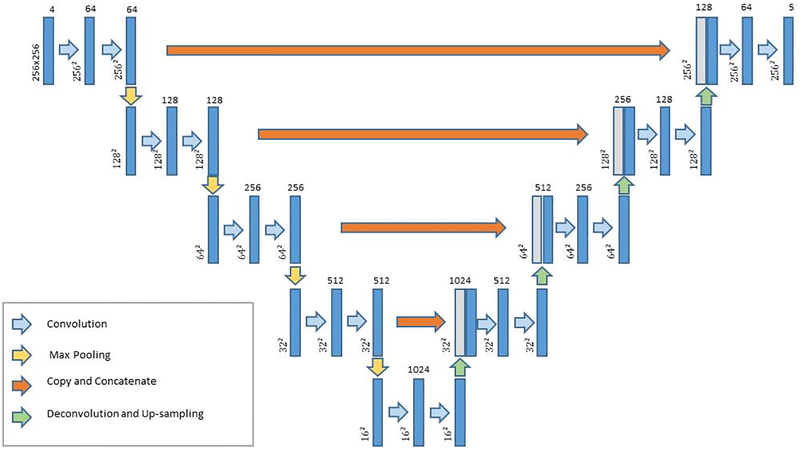
The multi-class U-net FCNN network used for segmentation is shown in Fig. 1. The network segmented the brain tissue into background and four classes: WM, GM, CSF, and T2-hyperintense WM lesions (T2 lesions). Convolution in the contracting path and deconvolution in the expanding path used 3 × 3 kernels with a 2 × 2 stride. The activation function was a rectified linear unit (ReLU). A 2 × 2 max pooling operation (stride 2) was used to reduce image size in the contracting path.

Figure 1.

Architecture of the convolutional neural network used for brain segmentation. The image dimension is denoted next to each layer, and the number of channels (features) is listed at the top.

The preprocessed PDw, T2w, T1w, and FLAIR images served as input to the FCNN. MRI automated processing (MRIAP), a validated software package that combines parametric and nonparametric techniques, [30] was used to segment the images. The MRIAP segmentation of CombiRx images were reviewed and validated/corrected by two experts with more than 15 and 25 years of experience in MS image analysis. This validated segmentation was used as the ground truth.

Five cases were not readily accessible in the database, and the analysis was performed on 1003 image sets acquired at baseline in the CombiRx trial. The data were randomly partitioned into training (60% of the scans), validation (20%), and test (20%) sets. For initializing the network weights, the Xavier algorithm was used [31].

To account for variations in the class sizes, the FCNN was trained using the multiclass Dice loss function [32]. The network training was performed with 500 epochs using the ADAM solver [33] for optimization with an initial learning rate of 10⁻⁴. Data augmentation was used during training, including horizontal and vertical flips, rotation, translation, and zooming. Training was implemented on the Maverick2 cluster at the Texas Advanced Computing Center (TACC) with four NVIDIA GTX 1080 Ti graphics processing unit (GPU) cards using the Python Keras library [34] and TensorFlow [35].

Cross Validation

To assess the model performance on unseen data, we performed cross validation using a leave-one-center-out approach. Data from 68 centers in the CombiRx dataset were randomly split into 17 partitions, each with 64 centers used for training and the remaining four centers used for testing. Network training was performed and performance was evaluated by calculating the mean, standard deviation, and 95% confidence intervals of the segmentation metrics over the different runs. Grouping 4 centers for testing was preferred over a single center because the former provides a more reliable test set size, and is computationally more efficient.

Evaluation

The class-specific accuracy was calculated by computing the Dice similarity coefficient (DSC) using Eq. (1):

$$DS{C}_K=\frac{2\times T{P}_K}{\left(F{P}_K+2\times T{P}_K+ F{N}_K\right)}$$ (1)

where TP_k, FP_k, and FN_k represent the number of true positive, false positive, and false negative classification of tissue class k, respectively. In addition, the volume of each tissue class was compared to the volume in the ground truth segmentation.

Next, the dependence of the lesion segmentation accuracy on the lesion size was assessed. Lesions were categorized, somewhat arbitrarily, into seven sets based on volume: 0–19 mm³; 20–34 mm³; 35–69 mm³; 70–137 mm³; 138–276 mm³; 277–499 mm³; and >500 mm³. The Dice coefficient and the lesion-wise true positive (TPR) and false positive (FPR) rates were calculated for each category.

RESULTS

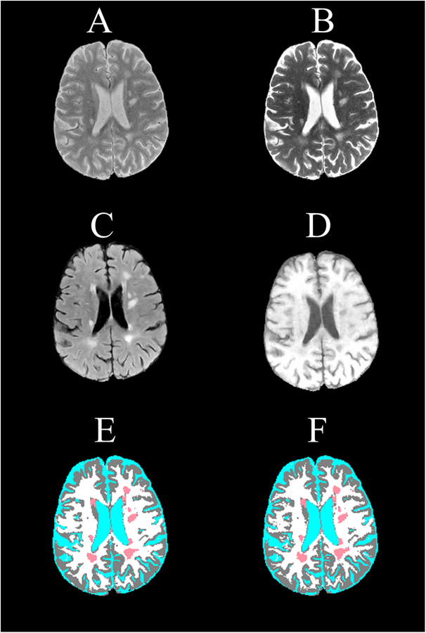
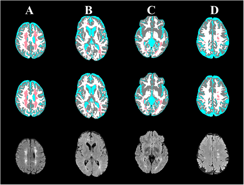
Quantitative assessment, based on DSC, showed high accuracy of FCNN segmentation on the test image set. The mean (95% confidence interval) DSC values were 0.95 (0.92–0.98) for WM, 0.96 (0.93–0.98) for GM, 0.99 (0.98–0.99) for CSF, and 0.82 (0.63–1.0) for T2 lesions. As an example, the input MRI images and the FCNN segmented image of one slice from an MS patient in the test set are shown in Fig. 2. For comparison, the corresponding ground truth segmented image is also shown. The high accuracy of the segmentation can be readily appreciated on this figure, which is also reflected in the measured DSC values of 0.91 (WM), 0.92 (GM), 0.98 (CSF), and 0.90 (T2 lesions). Figure 3 shows slices from another four different subjects showing the excellent correspondence between the FCNN output and the ground truth segmentation.

Figure 2.

Brain MRI images of an MS patient used as input to the segmentation CNN showing (A) proton density-weighted, (B) T2-weighted, (C) FLAIR, and (D) T1-weighted, and the corresponding (E) expert-validated MRIAP segmentation and (F) the CNN-generated segmentation. The tissue classes are color coded as white (WM), gray (GM), cyan (CSF), and light red (T2 lesions). DSC values of 0.90 (WM), 0.93 (GM), 0.99 (CSF), and 0.88 (T2 lesions) indicate high correspondence between the expert-validated and CNN-generated segmentations.

Figure 3:

Representative slices from expert-validated MRIAP segmentation (upper row) and corresponding CNN segmentation (middle row), and corresponding FLAIR images (lower row) of four MS patients. DSC of T2 lesions was 0.93, 0.85, 0.86, and 0.9 for cases A to D, respectively.

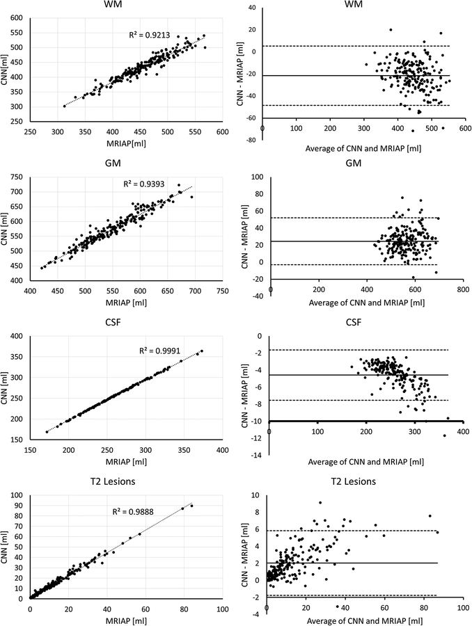
The concordance between the tissue volumes segmented by the FCNN and the ground truth for all patients in the test set along with the Bland-Altman plots is shown in Fig. 4. A high degree of agreement between the two segmentations is evident, with R² values of 0.92 (WM), 0.94 (GM), 1.0 (CSF), and 0.99 (T2 lesions). The Bland-Altman analysis shows only a small bias between the total tissue volumes estimated by the FCNN and the ground truth segmentations.

Figure 4:

(Left) Correlation between tissue volumes segmented by the CNN and the ground truth expert-validated MRIAP, and (right) the Bland-Altman plot. Very high correlation coefficients and small bias are observed.

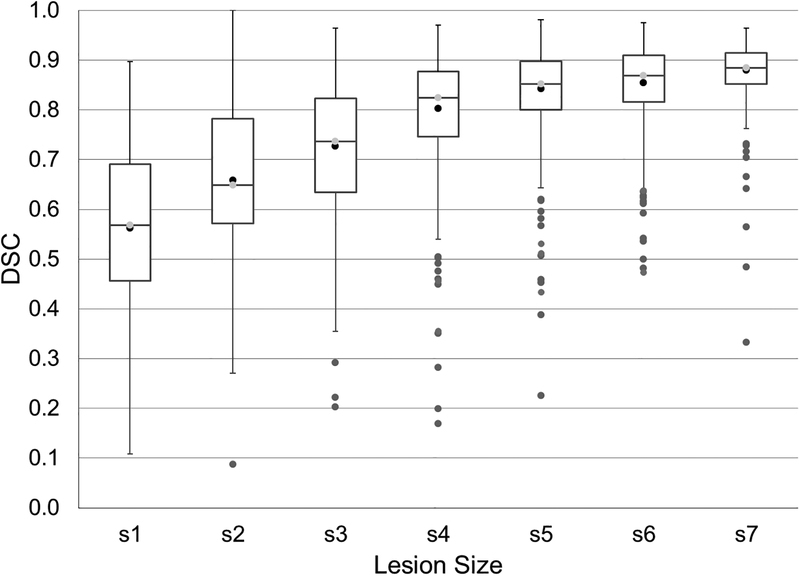
Dependence of the lesion segmentation accuracy on its size, as assessed by the DSC, is shown in Fig. 5, and the lesion-wise TPR and FPR are listed in Table 1. As expected, very small lesions were harder to segment. However, a remarkable TPR ≥ 91% and FPR ≤ 10% were achieved for all lesions larger than 70 mm³ (0.07 ml) in size. The average TPR and FPR over all lesions were 79% and 34%, respectively.

Figure 5:

The Dice similarity coefficient (DSC) stratified by lesion size shows progressive improvement in segmentation with increased lesion size.

Table 1.

Segmentation accuracy for different lesion sizes.

Lesion size (mm3)	Number of lesions (ground truth)	Number of lesions (FCNN)	TPR	FPR
0–19	3366	3673	0.66	0.60
20–34	1233	1118	0.76	0.30
35–69	1232	1089	0.87	0.16
70–137	912	861	0.91	0.10
138–276	654	628	0.95	0.03
277–499	364	333	0.96	0.01
>500	599	606	1.00	0.00
All	8360	8308	0.79	0.34

TPR, true positive rate; FPR, false positive rate.

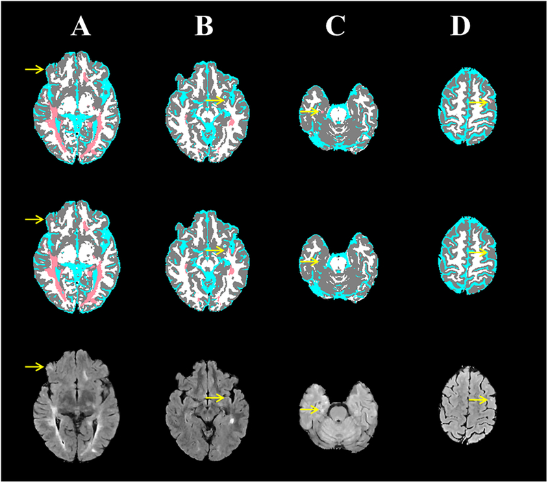
Despite the excellent segmentation, as reflected in the high values of DSC, TPR, and FPR values, DL models are not error-proof. Figure 6 shows examples where the segmentation from FCNN did not show complete agreement with the ground truth. In Case (A), the “ground truth” segmentation missed a small lesion that was successfully detected by the FCNN. However, Case (B) shows slight hyperintensity in subcortical white matter which was mistakenly segmented by the FCNN as a T2 lesion (false positive). Cases (C, D) show two cases in which subtle mediotemporal and subcortical lesions were missed by the FCNN.

Figure 6:

Four MS cases (columns) showing the brain segmentation from the expert-validated ground truth (top row) and the CNN (middle row), and corresponding FLAIR images (bottom row). (A) A small subcortical lesion that was detected by the CNN, but was missed in the “ground truth”. (B) A slight hyperintensity in subcortical white matter was mistakenly segmented by the CNN as a T2 lesion. (C) A mediotemporal lesion that was not detected with CNN. (D) A subcortical lesion that was missed by CNN.

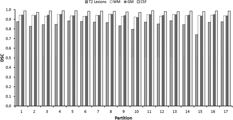
The results from the cross validation study, showing the tissue segmentation are summarized in Fig. 7. The results show relatively low variations in DSC between the center groups. The mean (95% confidence limits) of DSC were: T2 lesions, 0.85 (0.78–0.92); WM, 0.94 (0.92–0.95); GM, 0.94 (0.93–0.96); and CSF, 0.98 (0.97–0.99). Lesion-wise TPR and FPR were 76 (0.62–0.90) and 0.41 (0.33–0.50), respectively.

Figure 7:

Results of the leave-one-group-out cross validation showing performance of tissue segmentation in 17 independent runs. In each run, 64 sites were used for training and 4 sites were used for testing.

DISCUSSION

In this work, we trained and validated a DL model for brain segmentation using a large multi-center annotated MRI data. Through a hierarchy of features, DL can automatically learn both intensity distributions of the different tissues as well as the contextual information present in the data. In addition to lesion segmentation which is a conventional target in the published studies [13],[17], this work classified all the brain tissues. Accurate segmentation was obtained using FCNN as evidenced by the high degree of correspondence (Fig. 5) and high DSC scores of ≥ 0.95 for brain tissue, and 0.82 for T2 lesions. The high accuracy obtained in our results is attributed to the large multi-center image dataset and the use of four-dimensional multi-modal MRI information. Compared to other segmentation approaches, DL learns inherent image features and does not require extensive involvement from developers in selecting image features, nor does it require extensive post-processing to remove false-positive as is common in MS segmentation methods.

In this study training, validation, and testing was based on MRI data acquired from different centers and different scanners, and field strengths. This heterogeneity of the data is expected to provide more robust results as can be seen from the cross validation. However, all the data were acquired using the same MRI protocol. Applying the model developed in this work can be extended to data acquired using different imaging protocols using transfer learning [36], which benefits from the hierarchical features learned by a DL model trained on a large database. Fine tuning the model for protocol-specific factors can then be accomplished. This is currently a work-in-progress in our lab.

One of the challenges in DL-based segmentation is the availability of the annotated “ground truth” labels on large datasets. While manual segmentation can be obtained for small datasets, such segmentation is clearly impractical for large datasets such as those typically needed for a successful DL approach. Semi-automated methods such as that used in CombiRx eases the segmentation task by reducing the burden on the human expert role. However, natural intra- and inter-rater variabilities affect the quality of any segmentation. This, in part, explains the disagreement between the FCNN and the reference segmentation method observed in a few cases in this study. In many of these cases the FCNN appears to produce more plausible segmentation compared to the “ground truth”. This is attributed to misclassification in the initial automated segmentation and the tediousness of manual correction in large datasets. We excluded images of low quality from the dataset. Although quality acceptance procedures reduce the variability in the images, they are commonly implemented in almost all studies as low-quality images are more likely to produce unrealistic segmentation.

It would have been interesting to compare our results with those obtained using different automatic segmentation techniques. As articulated by Danelakis et al, [3], comparing segmentation methods is complicated by many issues such as the use of propriety software and/or image data, and the small number of images used for training. Moreover, segmentation methods vary in the number and type of images used as input. We therefore find the comparison to the ground truth segmentation the most plausible approach in this work. Unfortunately in medical images, the ground truth is seldom known. In our studies, ground truth was based on the validated semi-automatic segmentation which is further validated by an expert. We believe that this approach provided us accurate tissue volumes.

The Dice scores are most appropriate when applied in the same context and may not be the best performance metric. True and false positive rates may be more appropriate from the clinical perspective and were included in our results. However, the Dice coefficient is the most common metric reported in the segmentation literature, which we chose to adhere to in the present work.

The high Dice scores and the high TPR and low FPR indicate excellent overall segmentation accuracy. Yet, there were a small number of cases with relatively inaccurate segmentation. Therefore, in this study we have included examples with suboptimal segmentation to alert the research community that the network models, while powerful, are sometimes error prone.

While our dataset included 3D T1w images which provide excellent GM-WM contrast, we opted to use 2D T1w images because their geometries matched FLAIR and dual-echo FSE data. In addition, 2D acquisitions are more widely used in clinical practice.

We limited this study to the segmentation of brain tissues and WM T2 lesions in RRMS. Unfortunately, we could not include cortical lesions since the MRI protocol used in CombiRx was not designed for visualizing cortical lesions. Visualization of cortical lesions requires special MR pulse sequences such as the double inversion recovery sequence [37]. Future extension of the DL methods described here will address cortical lesions, and WM lesions with severe tissue destruction, known as black holes due to their low signal on T1-weighted MRI. Another application would be identifying active inflammatory lesions that can currently be only identified on post-contrast images. We have made the model used in this work publicly available (https://github.com/uthmri/Deep-Learning-MS-Segmentation).

In conclusion, we have demonstrated that fully convolutional neural networks can provide accurate segmentation of all brain tissues on a large multi-center study in multiple sclerosis. Finally we will deposit the scripts and other information about this model in a public repository for other interested investigators.

REFERENCES

- 1.Reich DS, Lucchinetti CF, Calabresi PA. Multiple Sclerosis. N. Engl. J. Med 2018; 378(2):169–180. Available at: 10.1056/NEJMra1401483. [DOI] [PMC free article] [PubMed] [Google Scholar]
- 2.Lublin FD, Cofield SS, Cutter GR, et al. Randomized study combining interferon and glatiramer acetate in multiple sclerosis. Ann. Neurol 2013; 73(3):327–340. [DOI] [PMC free article] [PubMed] [Google Scholar]
- 3.Danelakis A, Theoharis T, Verganelakis DA. Survey of automated multiple sclerosis lesion segmentation techniques on magnetic resonance imaging. Comput. Med. Imaging Graph 2018; 70:83–100. [DOI] [PubMed] [Google Scholar]
- 4.de Sitter A, Steenwijk MD, Ruet A, et al. Performance of five research-domain automated WM lesion segmentation methods in a multi-center MS study. Neuroimage 2017; 163:106–114. [DOI] [PubMed] [Google Scholar]
- 5.Egger C, Opfer R, Wang C, et al. MRI FLAIR lesion segmentation in multiple sclerosis: Does automated segmentation hold up with manual annotation? NeuroImage Clin 2017; 13:264–270. [DOI] [PMC free article] [PubMed] [Google Scholar]
- 6.Carass A, Roy S, Jog A, et al. Longitudinal multiple sclerosis lesion segmentation: resource and challenge. Neuroimage 2017; 148:77–102. [DOI] [PMC free article] [PubMed] [Google Scholar]
- 7.Ghribi O, Sellami L, Slima M Ben, et al. An Advanced MRI Multi-Modalities Segmentation Methodology Dedicated to Multiple Sclerosis Lesions Exploration and Differentiation. IEEE Trans. Nanobioscience 2017; 16(8):656–665. [DOI] [PubMed] [Google Scholar]
- 8.Valcarcel AM, Linn KA, Vandekar SN, et al. MIMoSA: An Automated Method for Intermodal Segmentation Analysis of Multiple Sclerosis Brain Lesions. J. Neuroimaging 2018. [DOI] [PMC free article] [PubMed] [Google Scholar]
- 9.Rocca MA, Comi G, Filippi M. The role of T1-weighted derived measures of neurodegeneration for assessing disability progression in multiple sclerosis. Front. Neurol 2017; 8:433. [DOI] [PMC free article] [PubMed] [Google Scholar]
- 10.Goodfellow I, Bengio Y, Courville A, Bengio Y. Deep learning MIT press; Cambridge; 2016. [Google Scholar]
- 11.LeCun Y, Bengio Y, Hinton G. Deep learning. Nature 2015; 521(7553):436. [DOI] [PubMed] [Google Scholar]
- 12.Ravi D, Wong C, Deligianni F, et al. Deep learning for health informatics. IEEE J. Biomed. Heal. informatics 2017; 21(1):4–21. [DOI] [PubMed] [Google Scholar]
- 13.Brosch T, Tang LYW, Yoo Y, et al. Deep 3D Convolutional Encoder Networks With Shortcuts for Multiscale Feature Integration Applied to Multiple Sclerosis Lesion Segmentation. IEEE Trans. Med. Imaging 2016; 35(4):1229–1239. [DOI] [PubMed] [Google Scholar]
- 14.Wachinger C, Reuter M, Klein T. DeepNAT: Deep convolutional neural network for segmenting neuroanatomy. Neuroimage 2018; 170:434–445. [DOI] [PMC free article] [PubMed] [Google Scholar]
- 15.Ghafoorian M, Karssemeijer N, Heskes T, et al. Location Sensitive Deep Convolutional Neural Networks for Segmentation of White Matter Hyperintensities. Sci. Rep 2017; 7(1):5110. [DOI] [PMC free article] [PubMed] [Google Scholar]
- 16.Moeskops P, Veta M, Lafarge MW, Eppenhof KAJ, Pluim JPW. Adversarial training and dilated convolutions for brain MRI segmentation In: Deep Learning in Medical Image Analysis and Multimodal Learning for Clinical Decision Support Springer; 2017:56–64. [Google Scholar]
- 17.Valverde S, Cabezas M, Roura E, et al. Improving automated multiple sclerosis lesion segmentation with a cascaded 3D convolutional neural network approach. Neuroimage 2017; 155:159–168. [DOI] [PubMed] [Google Scholar]
- 18.Dolz J, Desrosiers C, Ben Ayed I. 3D fully convolutional networks for subcortical segmentation in MRI: A large-scale study. Neuroimage 2018; 170:456–470. [DOI] [PubMed] [Google Scholar]
- 19.Hoseini F, Shahbahrami A, Bayat P. AdaptAhead Optimization Algorithm for Learning Deep CNN Applied to MRI Segmentation. J. Digit. Imaging 2018:1–11. [DOI] [PMC free article] [PubMed] [Google Scholar]
- 20.Kushibar K, Valverde S, González-Villà S, et al. Automated sub-cortical brain structure segmentation combining spatial and deep convolutional features. Med. Image Anal 2018; 48:177–186. [DOI] [PubMed] [Google Scholar]
- 21.Rachmadi MF, Valdés-Hernández M del C, Agan MLF, et al. Segmentation of white matter hyperintensities using convolutional neural networks with global spatial information in routine clinical brain MRI with none or mild vascular pathology. Comput. Med. Imaging Graph 2018; 66:28–43. [DOI] [PubMed] [Google Scholar]
- 22.Charron O, Lallement A, Jarnet D, et al. Automatic detection and segmentation of brain metastases on multimodal MR images with a deep convolutional neural network. Comput. Biol. Med 2018; 95:43–54. [DOI] [PubMed] [Google Scholar]
- 23.Ronneberger O, Fischer P, Brox T. U-Net: Convolutional Networks for Biomedical Image Segmentation. In: International Conference on Medical image computing and computer-assisted intervention; 2015:234–241. [Google Scholar]
- 24.Laukamp KR, Thiele F, Shakirin G, et al. Fully automated detection and segmentation of meningiomas using deep learning on routine multiparametric MRI. Eur. Radiol 2018:1–9. [DOI] [PMC free article] [PubMed] [Google Scholar]
- 25.Lindsey JW, Scott TF, Lynch SG, et al. The CombiRx trial of combined therapy with interferon and glatiramer cetate in relapsing remitting MS: Design and baseline characteristics. Mult Scler Relat Disord 2012; 1(2):81–86. [DOI] [PMC free article] [PubMed] [Google Scholar]
- 26.Narayana PA, Govindarajan KA, Goel P, et al. Regional cortical thickness in relapsing remitting multiple sclerosis: A multi-center study. NeuroImage Clin 2013; 2(1):120–131. [DOI] [PMC free article] [PubMed] [Google Scholar]
- 27.Perona P, Malik J. Scale-space and edge detection using anisotropic diffusion. IEEE Trans. Pattern Anal. Mach. Intell 1990; 12(7):629–639. [Google Scholar]
- 28.Gerig G, Kbler O, Kikinis R, Jolesz FA. Nonlinear Anisotropic Filtering of MRI Data. IEEE Trans. Med. Imaging 1992; 11(2):221–232. [DOI] [PubMed] [Google Scholar]
- 29.Nyúl LG, Udupa JK, Zhang X. New variants of a method of MRI scale standardization. IEEE Trans. Med. Imaging 2000; 19(2):143–150. [DOI] [PubMed] [Google Scholar]
- 30.Sajja BR, Datta S, He R, et al. Unified approach for multiple sclerosis lesion segmentation on brain MRI. Ann Biomed Eng 2006; 34(1):142–151. [DOI] [PMC free article] [PubMed] [Google Scholar]
- 31.Glorot X, Bengio Y. Understanding the difficulty of training deep feedforward neural networks. In: Proceedings of the thirteenth international conference on artificial intelligence and statistics; 2010:249–256. [Google Scholar]
- 32.Isensee F, Kickingereder P, Wick W, Bendszus M, Maier-Hein KH. Brain Tumor Segmentation and Radiomics Survival Prediction: Contribution to the BRATS 2017 Challenge. In: International MICCAI Brainlesion Workshop; 2017:287–297. [Google Scholar]
- 33.Kingma DP, Ba JL. Adam: A method for stochastic optimization. In: International Conference on Learning Representations (ICLR); 2015. [Google Scholar]
- 34.Keras Chollet F.. 2015. Available at: https://github.com/keras-team/keras.
- 35.Abadi M, Barham P, Chen J, et al. TensorFlow: A System for Large-Scale Machine Learning TensorFlow: A system for large-scale machine learning. In: 12th USENIX Symposium on Operating Systems Design and Implementation (OSDI ‘16); 2016. [Google Scholar]
- 36.Torrey L, Shavlik J. Transfer learning In: Handbook of Research on Machine Learning Applications and Trends: Algorithms, Methods, and Techniques IGI Global; 2010:242–264. [Google Scholar]
- 37.Nelson F, Poonawalla AH, Hou P, et al. Improved identification of intracortical lesions in multiple sclerosis with phase-sensitive inversion recovery in combination with fast double inversion recovery MR imaging. AJNR Am J Neuroradiol 2007; 28(9):1645–1649. [DOI] [PMC free article] [PubMed] [Google Scholar]