Clonal Decomposition and DNA Replication States Defined by Scaled Single-Cell Genome Sequencing

Summary

Accurate measurement of clonal genotypes, mutational processes, and replication states from individual tumor-cell genomes will facilitate improved understanding of tumor evolution. We have developed DLP+, a scalable single-cell whole-genome sequencing platform implemented using commodity instruments, image-based object recognition, and open source computational methods. Using DLP+, we have generated a resource of 51,926 single-cell genomes and matched cell images from diverse cell types including cell lines, xenografts, and diagnostic samples with limited material. From this resource we have defined variation in mitotic mis-segregation rates across tissue types and genotypes. Analysis of matched genomic and image measurements revealed correlations between cellular morphology and genome ploidy states. Aggregation of cells sharing copy number profiles allowed for calculation of single-nucleotide resolution clonal genotypes and inference of clonal phylogenies and avoided the limitations of bulk deconvolution. Finally, joint analysis over the above features defined clone-specific chromosomal aneuploidy in polyclonal populations.

Graphical Abstract

Highlights

• •Scaled method and resource of > 50K single-cell whole genomes from diverse cell types
• •Clonal merging can resolve clone specific mutations to single-nucleotide level
• •Image analysis of single cells permits correlation of morphology and genome features
• •Clonal replication states and rare aneuploidy patterns of single cells measured

A high-throughput method for amplication-free single-cell whole-genome sequencing can be scaled up to analyze tens of thousands of cells from different tissues and clinical sample types and identifies replication states, aneuploidies, and subclonal mutations.

Introduction

Large-scale single-cell whole-genome analysis has the potential to yield new insights into the molecular dynamics of cellular populations, currently a frontier of tumor biology research. However, technological advances in single-cell genomics have lagged those of transcriptomics (Macosko et al., 2015, Ziegenhain et al., 2017), due in part to physical limitations of capturing DNA with even coverage across the genome (Gawad et al., 2016). Measuring single-cell genomes at scale in tissues and cell populations will greatly advance clonal decomposition of malignant tissues, studying properties of negative selection, resolving rare cell population genotypes and identifying DNA replication states of individual cells, all of which are hard to measure when cellular information is destroyed in bulk sequencing. Several amplification-based methods have been described (Navin et al., 2011, Zong et al., 2012, Hou et al., 2012, Ni et al., 2013, Gawad et al., 2014, Lohr et al., 2014, Wang et al., 2014, Baslan et al., 2012), including degenerate oligonucleotide-primed PCR (DOP-PCR), multiple displacement amplification (MDA) and multiple annealing- and looping-based amplification cycles (MALBAC); however, amplification introduces both coverage and polymerase bias into sequences (Gawad et al., 2016), leading to lower fidelity representations of the genome and analytical scenarios where duplicate sequences cannot be easily resolved. The recently introduced single-cell combinatorial indexed sequencing (SCI-seq) aims to increase the throughput of single-cell sequencing but is limited by its high duplication rate and relatively low coverage breadth (Vitak et al., 2017).

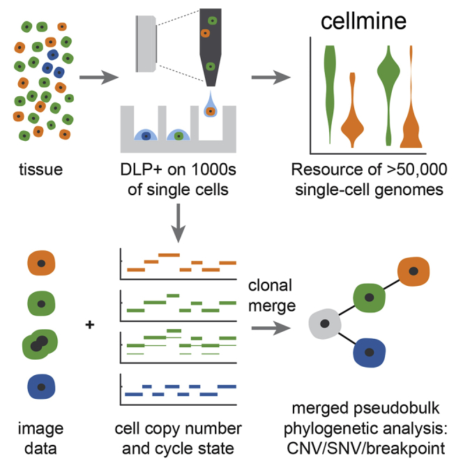
Previously, we showed that direct DNA transposition single-cell library preparation (DLP) performed with microfluidic devices reduced the biases relative to pre-amplification-based approaches (Zahn et al., 2017). Despite the performance of microfluidic-based DLP (M-DLP) analysis, the use of custom microfluidic devices presents an obstacle to adoption in many labs and also places limits on scalability due to fabrication constraints. Microfluidic devices also impose constraints on cell size, with large cells clogging channels and very small cells passing through traps, unless devices are customized for the cell type. Similar limitations on cell size apply to some droplet-based methods. To address these limitations, we have developed and optimized an alternative and much higher-throughput direct transposition single-cell whole-genome sequencing approach, referred to here as DLP+, based on commodity high-density nanowell arrays and picoliter volume piezo-dispensing technology available “off the shelf” (Figure 1). A unique and significant advantage of DLP+ is the ability to capture high-resolution microscopy images of objects prior to dispensation using an integrated camera and transparent dispensing nozzle. The camera and real-time software perform image-based quality control, allowing for active selection of single cells, thereby avoiding the sequencing of doublet cells or debris. We show that optimized DLP+ enables robust and scaled analysis of tens of thousands of cells per experiment across various tissue types. From a resource of 51,926 DLP+ sequenced single cells, we show how DLP+ data can be used to identify clonal populations and their genomic features, properties of individual cells including replication state and chromosomal mis-segregation, and relationships between genomic and morphological properties.

Figure 1.

Concept Schematic of the Experimental and Computational Processes for DLP+

(A) Cell isolation and lysis.

(B) Open-array library construction. DLP+ libraries from unamplified single cells are built by carrying the chip through a series of reagent addition, spin, seal, and heat incubation steps.

(C) Pooled recovery for sequencing.

(D) Computational pipeline workflow for single-cell genome data management, alignment, and post-processing.

Results

A Resource of Diverse, Annotated, Single-Cell Genomes Generated with Scalable Open Array Transposon-Mediated DNA Sequencing

Scalable Single-Cell Library Preparation in Open Nanoliter Wells

To scale amplification-free transposon-based single-cell genome sequencing to thousands of cells per library, we implemented a new platform called DLP+ by using commodity off the shelf components, principally comprised of a contactless piezoelectric dispenser (sciFLEXARRAYER S3 and cellenONE, Scienion) and open nanowell arrays (TakaraBio SmartChip; Figure 1, Figure S1A). Key elements include a large number of freely programmable reagent steps, real-time imaging, and object recognition allowing arrayed dispensing and doublet removal, bypassing limitations of Poisson loading. Details of the platform are fully described in Figure S1. Since imaging occurs before the library preparation reagents are spotted, doublets, empty wells, or cells with contamination are excluded from library preparation at two steps, during nozzle imaging and subsequently in a well-imaging step (Figure 1A, Figure S1E). The final libraries are pooled during recovery (Figure 1C) and sequenced at the desired coverage depth by using standard Illumina protocols and HiSeq instruments, yielding raw, indexed FASTQ data for analysis and interpretation.

Figure S1.

Spotter Setup and Single-Cell Isolation, Related to Figure 1 and STAR Methods, Method Details

(A) Spotting robot setup featuring: (I) nanowell open-array chip located on customized chip-holder, (II) wash-solution reservoir, (III) active fresh-water wash station, (IV) dispensing nozzle, (V) droplet camera, (VI) chilled target holder.

(B) Brightfield image of the dispensing nozzle. Orange arrow highlights ejected droplet which can range from 300- 550 pL in size depending on instrument settings.

(C) Overlay of a brightfield image showing the dispensing nozzle and the mapping density of detected cells. Green dots indicate ejected cells; blue dots indicate cells that were again detected after ejecting a single droplet; dotted blue line shows boundary of cell ejection area/volume; dotted orange line indicates sedimentation boundary.

(D) Automated imaging permits the identification of single cells and target deposition into a nanowell. Cells were deposited if a single cell was detected in the ejection area and no particle was present in the sedimentation area. Orange arrow highlights selected single cell for deposition. e Brightfield image showing contaminating debris (orange arrow).

(F) Montage of 186 fluorescent images of isolated single cells in the bottom of a nanowell using the cellenONE software. Images are aligned according to the array layout.

(G) Left image: Nozzle image of an example doublet cell identified at spotting. Right image: CFSE stained plate image of the nanowell corresponding to the doublet, identified by the image processing SmartChipApp.

To scale analysis and quality control of DLP+ data analysis, we developed and deployed open-source, cloud-compatible software infrastructure. Requirements for the system included automation of per cell quality assessment, interactive visualization for efficient quality control (QC), and managing the storage and analysis of large amounts of data and metadata produced by our sequencing experiments. The system includes two databases: Colossus for tracking per cell metadata and Tantalus for tracking raw and processed sequencing datasets and metadata for associated analyses. Raw sequencing data are processed using the single-cell pipeline, a set of workflows for producing QC and variant data built upon a cloud-capable workflow engine. The pipeline implements workflows for whole-genome alignment, Hidden Markov Model-based copy number inference including ploidy estimation, and calculation of SNVs, breakpoints, and allelic measurements. A key feature of the single-cell pipeline is an 18-feature classifier of library quality trained on 20,000 manually curated libraries producing a quality score (QS) metric for efficient quality assessment of DLP+ libraries (Figures S2C and S2D). Results from the single-cell pipeline are loaded into Montage, a web-based, interactive data-visualization platform for QC and data exploration. Montage allows for the construction of dashboards for interactive exploration of large amounts of multidimensional data served by an Elasticsearch backend. A key feature of Montage is linked charts; selection or filtering of datapoints in one chart propagates to all other charts of the same data, facilitating novel data-exploration-use cases without requiring development of bespoke visualization software. Single-cell data from this report may be visualized in a Montage instance available at https://www.cellmine.org. The details of the quality score classifier derivation, analysis pipeline, and software downloads are in the STAR Methods and Data S1.

Figure S2.

Optimization of DLP+ Single-Cell Whole-Genome Sequencing Library Construction for the Open-Array Format, Related to Figure 2

Examples of (A) high-quality and (B) poor quality single-cell genome libraries from a diploid GM18507 lymphoblastoid (male) cell line. Colors correspond to integer HMM copy number states (Ha et al., 2012); black lines indicate segment medians.

(C) Random forest classifier feature importance, total mapped reads is of highest importance. Definitions of the features are in methods.

(D) OC from 10 ten-fold cross-validation on Random Forest (AUC 0.997)

(E) Quality score distribution over GM18507 cells of (i) the original MF-DLP data (Zahn et al., 2017)), (ii) lysis buffer types, (iii) Tn5 concentrations and increased lysis presoak times (iv) on-chip storage of isolated cells and nuclei that were dispensed into nanowells and stored either overnight or for 63 days prior to lysis and library construction, and (v) cell state (live or dead). Numbers of cells are indicated above each violin plot, where black lines show medians and dots indicate individual cells (green circle = live, orange diamond = dead, gray square = no cell state data). Grey background indicates where cells underwent heat lysis immediately after lysis buffer addition, and blue background indicates cells kept in lysis buffer for 19 h at 4°C before heat lysis.

(F) Effect of cell dispensing method on total mapped reads, with active selection (cellenONE, spotted in a block of wells or a scatter pattern) or passive limiting dilution dispensing. Black lines show median.

(G) Effect of protease concentration on cells. Quality scores of single-cell libraries built with a low, medium, or high concentration of protease in the lysis buffer and lysed for either 2 or 19 h, followed by library construction with a range of protease concentrations.

(H) Distribution of coverage breadth of bootstrap sampling of GM18507 libraries using a 2 h and overnight presoak lysis compared to a microfluidic device (MF-DLP ($n=$ 122, (Zahn et al., 2017)), DLP+ 2 h ($n=$ 148), DLP+ overnight ($n=$ 133).

(I) The effect of lysis time on coverage breadth of merged single-cell genomes. Bootstrap sampling of single-cell GM18507 libraries prepared using a 2 h and overnight cold lysis conditions; DLP+ 2 h ($n=$ 148), DLP+ overnight ($n=$ 133), MF-DLP Zahn et al. (2017) ($n=$ 122). Single-cell libraries were downsampled to a similar median coverage depth. Boxplots show median and quartiles, the whiskers show the remaining distribution, and dots indicate outliers. Lorenz curves shows coverage uniformity for merged single-cell genomes. Curves are median merged genomes. Experimental condition and number of merged cells are indicated in the plot. Dotted black line indicates perfectly uniform genome.

(J) Distribution of fraction duplicate reads for GM18507 cells (2.2 nL Tn5, $n=$ 587 (green); 3.5 nL Tn5, $n=$ 571 (blue)) and on a microfluidic device ($n=$ 141, (Zahn et al., 2017) (yellow)). The top column labels state the numbers of cells per condition.

(K) Fraction duplicate reads versus coverage breadth of deeply sequenced GM18507 libraries (3.5 nL Tn5, $n=$ 571), 10 HiSeqX lanes) with low quality ($<$ 0.75) and high quality ($\ge$ 0.75) indicated.

(L) GC bias of GM18507 libraries as a function of Tn5 concentrations and 8 or 11 PCR amplification cycles.

(M) Lorenz curves showing genome-wide coverage uniformity of merged single-cell libraries over Tn5 concentrations and 8 or 11 PCR amplification cycles (downsampled to 64 cells per experimental condition). Dotted straight black line indicates perfectly uniform genome.

(N) Effect of Tn5 concentration and PCR cycles time on coverage of merged single-cell genomes. Bootstrap sampling of single-cell GM18507 libraries prepared using a range of Tn5 concentrations and PCR indexing cycles on the open-array and compared to the MF-DLP dataset (7); DLP+ 2.2 nL Tn5, 8 PCR ($n=$188), 3.5 nL Tn5, 8 PCR ($n=$ 190), 6.5 nL Tn5, 8 PCR ($n=$ 197), 2.2 nL Tn5, 11 PCR ($n=$ 198), and MF-DLP (7) ($n=$ 122). Single-cell libraries were downsampled to a similar median mean coverage depth. Coverage depth and coverage breadth are shown in boxplots.

Biological and Physical Determinants of High-Quality DLP+ Library Construction

To establish experimental conditions that optimized DLP+, we initially applied the same reaction conditions from M-DLP (Zahn et al., 2017). This resulted in many poor-quality libraries due to: (1) alignments for which interpretable, integer state copy number profiles could not be inferred with low-quality score values and (2) failed libraries where coverage was low or absent (Figures S2A and S2E; 1 nL G2 buffer). We therefore optimized the physical reaction determinants of high-quality libraries by using quality score as a benchmark by systematically varying multiple factors: cell lysis volume and buffer type, transposase (Tn5) concentration, post-indexing PCR cycles, cell lysis/DNA solubilization time, and cell viability state. Each of these proved to have measurable impact on performance (Figure S2), and interactions between each parameter were determined. After optimization, we compared reaction conditions relative to the GM18507 M-DLP dataset (Zahn et al., 2017) by using bootstrapped subsampling of libraries to comparable read depths. We found by using optimized reaction conditions that genome coverage was as good or better with DLP+ (see Data S1 for details) but with a substantial increase in throughput over the MF-DLP method, scaling from hundreds to thousands of cells (Figure S2E, Data S1).

We next applied optimized DLP+ across a range of different tissue and cell types including cell lines, human breast cancer patient-derived xenograft (PDX) samples, a mouse model of synovial sarcoma (SS), patient tumor samples from frozen follicular lymphomas (FL), a diagnostic fine-needle aspirate (FNA) specimen from a breast cancer patient, and nuclei from flash frozen tissues, generating a reference resource of high-quality annotated single-cell genomes (Figure 2, Table S2). Cells from these samples range in size from 5 microns to 80 microns and included cells fresh from culture (cell lines), cells isolated from cryopreserved tissues (breast PDX, FL), and cells from dissociated primary tumor material. The DLP+ process allows for dead cells to be selectively excluded from library construction based on their fluorescent staining. For the purposes of this study, we included dead cells to allow for evaluation of the effect of cell viability on successful library construction in different tissue types and to provide a full reference set of genomes in differing biological states.

Figure 2.

DLP across Different Tissue Types Split by Viability: Live Cells ($n=$ 35,973, Green) and Dead Cells ($n=$ 8,877, Orange)

(A) Violin plots showing the quality score of single-cell libraries across various tissue types, split by cell viability status (live or dead), with number of cells shown above the violin. Black lines show median.

(B) Fraction of successful cells in a sample (quality > 0.75), split by cell viability. The size of the bubble represents the total number of successful cells. Violin and bubble colors indicate cell viability.

(C) Example single-cell copy number profiles from cell lines, breast PDX, follicular lymphoma, and mouse synovial sarcoma. Colors correspond to integer HMM copy number states; black lines indicate segment medians. Arrows highlight regions of complex copy number change.

We applied the quality score classifier to 51,926 DLP+ libraries sequenced from cells and nuclei as described above and defined successful high-quality libraries as those with quality score $\ge$ 0.75. We observed that 65.0% of cells labeled as live ($n=$ 25,270/38,705) produced high-quality single-cell genome sequences. Per sample, the live cell success rates ranged from 30.6% to 96.0% with a median of 73.3%, with 28/33 samples having a live cell success rate over 50% (Figures 2A and 2B). For tissue and cell line samples where both live and dead cells were included ($n=$ 32), dead cells had significantly lower quality scores than live cells, accounting for sample as a covariate (nested ranks test p value < 10^-4). Nevertheless, 36.0% of cells labeled as dead ($n=$ 3,776/10,577) produced high-quality libraries. Low-quality (quality score $\le$ 0.75) dead cells were characterized by low read count (median per cell read count 15,106) but did not exhibit representation bias or non-integer copy states. Finally, the success rate for nuclei was 66.0% ($n=$ 972/1,468), and quality metrics including quality score, total mapped reads, duplicate reads, and integerness were comparable between cells and nuclei prepared in parallel from the same sample (Figures S3A and S3C). Nuclei were intermixed with cells when clustering both cell and nuclei copy number data obtained for the same sample (Figure S3B), providing further evidence that nuclei produce libraries with quality and characteristics similar to cells. Notably, high-quality libraries can identify highly aneuploid genome states, including complex rearrangements (Figure 2C) in a similar manner to DLP. Taken together, the above data illustrate the scalability and versatility of DLP+ single-cell whole-genome sequencing.

Figure S3.

DLP+ Produces High-Quality Libraries from Cells and Nuclei, while Dead Cells Drop Out with Low Read Count, Related to Figure 2

(A) Quality score distribution of optimized single-cell libraries, split by dead cells, live cells, and nuclei shows live cells and nuclei have a similar distribution, while dead cells have lower quality. Total mapped reads distribution (orange is cells with quality score less than 0.75, and green is cells with quality score higher than 0.75), cells with low read counts have low-quality score, vertical line represents 125,000 reads.

(B) Heatmap of copy number profiles from cells and nuclei shows that cells (green in side bar) and nuclei (blue) cluster together using hierarchical clustering.

(C) Sequencing metrics of single-cell and single-nucleus libraries produced from the same samples.

(D) Example copy number profile from a nucleus and a cell derived from the same sample showing the same copy number clone type.

Ascertainment of Clone Specific Single-Nucleotide Resolution Mutations and Phylogenies

Single-cell sequencing techniques promise to provide more accurate measurement of clonal genotypes and clone proportions in cancer samples thereby obviating cumbersome and error-prone bulk tissue computational deconvolution methods. This in turn facilitates accurate phylogenetic reconstruction of major clones in a cancer. An important practical trade-off is the coverage per cell of genome sequenced against the number of cells from a population. We hypothesized that large numbers of DLP+ single-cell genomes sequenced at low coverage, could be leveraged to determine clonal populations and subsequently infer clone-specific nucleotide resolution somatic events including SNVs, allele-specific copy number and rearrangement breakpoints plus phylogenetic trees computed over these events. To address this, we developed an analytic workflow which first predicted somatic SNVs, and breakpoints on a merged dataset where all cells were collapsed into a “pseudo-bulk” genome. We then clustered single cells into cell subsets by their copy number profiles and measured the presence/absence of somatic, and rearrangement breakpoints in each clone. Given measurements of variants per clone, we then calculated allele specific copy number per clone and inferred phylogenetic evolutionary histories given SNVs, breakpoints, and copy number profiles.

To exemplify this approach, we generated 1,966 DLP+ libraries from 3 clonally related high-grade serous (HGS) ovarian cancer cell lines derived from the same patient, sourced from one primary tumor and two relapse specimens. On cells with > 500,000 reads ($n=$ 1,542 cells retained) and quality score > 0.5 ($n=$ 1,345 cells retained) we used dimensionality reduction and clustering (Data S1) to identify 9 cell subsets with shared copy number profiles as a first approximation to clones (subsets with ≥ 50 cells, 891 cells retained). The 9 clones ranged in size from 62 to 145 cells with a median coverage depth of 15x (Figure S5E and S5H).

Figure S5.

Pseudo-bulk Supplementary Analysis Showing Comparison of Pseudo-bulk SNV Detection between 2 and 4 Lanes of Sequencing; Relative Performance of Bulk Deconvolution for In-silico Mixtures, Related to Figure 3

(A) Heatmap of the number of SNVs (values in heatmap) that are detected in the 2 lane dataset (x axis) versus the 4 lane dataset (y axis) for three related ovarian cell lines.

(B) Counts of the total number of reads (sum of reference and alternate allele, x axis) for SNVs detected in the 2 lane dataset for three ovarian cell lines, split by total copy number of the encompassing region (y axis) and the phylogenetic status of each SNV (hue).

(C) Similar to b, for the 4 lane ovarian cell line dataset.

(D) Total clone fraction error (y axis) as boxplots for the 2 and 3 clone mixtures (y axis, n = 6, n = 9) for each method.

(E) Proportion of mixtures for which the number of predicted clones was correct (y axis) for the 2 and 3 clone mixtures (y axis) for each method.

(F) Mean correlation between predicted and clone copy number (y axis) for the 2 and 3 clone mixtures (y axis) for each method.

(G) Coverage in reads reference nucleotide for OV2295 clones.

(H) Cell count for OV2295 clones. i Histogram of the proportion of SNVs with 1 or more covering reads across cells.

(J) Distribution of log read counts per haplotype block as boxplots for OV2295 clones.

(J) Distribution of log read counts per SNV as boxplots for OV2295 clones.

(L) Distribution of log unique read counts per detected breakpoint for OV2295 clones.

For each clone, we computed clone-specific features including total copy number (Figure 3A), allele-specific copy number, SNVs and breakpoints. For allele specific copy number, we inferred haplotype blocks from germline polymorphisms (inferred from matched bulk normal genome) using Shape-IT (Delaneau et al., 2011) and the 1000 Genomes phase 2 reference panel. Across the 9 clones, high-quality allelic measurements were available for 92%–94% of the genomic bins based on a threshold of at least 1 haplotype block per bin and 100 reads per haplotype block per clone. Clone-specific haplotype block allele ratios coincided with fractional values that could easily be matched to genotypes consistent with clone specific copy number calls. For each clone, we thus fit a straightforward HMM to infer minor copy number based on haplotype block read counts and total copy number (Figure 3B). By way of example, total copy number and minor allele fraction for clone E (Figures 3A and 3B, 145 cells) is consistent with a whole-genome duplication (WGD) event. Chromosomes 1, 7, 10, and 11 all harbor 4 copies and a minor allele fraction near 0.5. Furthermore chromosomes 2, 5, and 9 all contain segments with 3 copies and minor allele fraction of 0.33. These events are consistent with single copy loss from a WGD event. By contrast, chromosomes 3, 4, 6, and 12 all harbor segments with 5 copies and minor allele fraction of 0.4 consistent with a single copy gain (e.g., AAABB) after WGD. Additionally, DLP+ allows for the resolution of clone specific focal amplifications such as the 4-copy segment of chromosome 13 specific to the clone 1, 8 branch of the phylogeny, an event that would be difficult to characterize from merged data of OV2295. Finally, we interpreted segments with minor allele fraction of 0 as loss of heterozygosity events. These are evident directly from the data: for example, chromosome 17, known to be homozygous in nearly 100% of HGS ovarian cancers, is unambiguously centered at 0 minor allele fraction.

Figure 3.

Features from Merging of Clones of OV2295, OV2295(R2), and TOV2295(R) Cell Lines Based on Single-Cell CNV ($n=$ 891)

(A) Raw total copy number for clone E (y axis) across the genome (x axis) colored by inferred total copy number.

(B) Minor allele frequency of clone E (y axis) across the genome (x axis) with inferred minor copy number ratio (minor copy number / total copy number) shown as blue lines.

(C) Presence of breakpoints (y axis) in each clone (x axis).

(D) Presence and state of SNVs (y axis) in each clone (x axis) with SNVs with no coverage in a clone shown in red, heterozygous and homozygous SNVs as determined by reference and alternate allele counts shown in dark and light blue respectively.

(E) Cell counts per clone per sample.

(F) Reduced dimensionality representation of n = 1,345 cells passing preliminary filtering, with cells excluded by additional filtering in gray, as calculated using UMAP.

(G) Correlation between counts of breakpoints and SNVs on the branches of the identically structured phylogeny inferred for both variant types. The shaded region represents the 95% confidence interval of the regression line.

(H) Phylogenetic tree with branch lengths calculated as counts of SNVs originating on each branch.

We further explored the inferred clusters using both SNVs and breakpoints. We used mutationSeq (Ding et al., 2012) and Strelka (Saunders et al., 2012) to identify SNVs across the 9 clones, and maximum likelihood to infer a phylogenetic tree relating the inferred clones (Figure 3D and 3H). As expected, each of the 3 samples formed a distinct clade in the phylogeny.

A total of 14,068 SNVs passed thresholding of which 84% fit perfectly with the inferred phylogenetic tree, 28% predicted as ancestral, 9% clone specific and the remaining 63% clade specific. Ancestral mutations with significant impact were found in TP53 (584T > C), FOXP2, and SUGCT. Clade specific mutations with significant impact were found in ZHX1, HTR1D and INSL4. We then used an orthogonal method (hierarchical clustering) to infer a phylogeny from breakpoints inferred using deStruct (McPherson et al., 2017a) (Figure 3C). A total of 538 passed thresholding of which 88% fit perfectly with the inferred phylogeny. By maximum parsimony, 15% breakpoints were predicted as ancestral, 11% as clone specific, and the remaining 73% as clade specific, mimicking the rankings of SNV phylogenetic class proportions. The topology of the breakpoint phylogeny was identical to the SNV phylogeny and counts of breakpoints and SNVs along specific branches were highly correlated (Figure 3, p value < 2.1∗10⁻⁷ Spearman rank). The OV2295 datasets are available at zenodo (https://doi.org/10.5281/zenodo.3445364).

The phylogenetic congruency of SNVs and breakpoints suggest the cell subsets inferred from copy number profiles represent accurate genomic clones with unambiguous genomic structure to a first approximation. While many methods have been developed for whole-genome clonal deconvolution (Carter et al., 2012, Nik-Zainal et al., 2012, Fischer et al., 2014, Ha et al., 2014, Oesper et al., 2014, Deshwar et al., 2015, McPherson et al., 2017b), most suffer from unidentifiability challenges induced by the combinatorial interaction between tumor content, cancer cell fraction, baseline ploidy, and copy number genotype. We generated in-silico mixtures of cells, sampling from the three original ovarian cancer source samples in pre-specified proportions. We then compared ReMixT, THeTA2 and CloneHD to clustering applied to DLP+ copy number profiles (see STAR Methods). Bulk deconvolution exhibited poor performance in predicting: (1) clonal fraction (Figure S5D), (2) number of clones in the mixture (Figure S5E), and the (3) copy number architecture of each clone (Figure S5E) relative to single-cell DLP+, establishing that single-cell DLP+ is more effective in deconvolving copy number clones than bulk methods.

We next executed a proof of principle experiment, establishing efficacy of DLP+ for clone identification and analysis in a clinical diagnostic setting, using limited material from a fine needle aspirate (FNA) biopsy. FNA sampling is less invasive than wide bore core biopsy procedures; however, the number of cells obtained is often more limited. We applied DLP+ to an FNA of a breast cancer (stage cT2N0, triple negative, BRCA2+/− germline, see STAR Methods). We then reconstructed copy number clonal architecture of the malignant cells and derived the reference germline genome from cells with diploid copy number—all from a single FNA sample (Figure 4). Clustering analysis yielded 62 cells with diploid copy number, and 3 aneuploid populations comprising 220 cells. Adopting the diploid cells as a germline reference cell population for comparison, we extracted heterozygous germline SNPs, inferred haplotype blocks, and computed allele specific copy number from each malignant clone. Our analysis produced copy number and LOH profiles for 3 tumor clones in the FNA (Figure 4), allowing us to identify ancestral clonal amplifications in MCL1, MYC and CCNE1, clone-specific amplifications of RAD18 and RAB18, and clonal LOH of BRCA2 coincident with a germline loss of function mutation.

Figure 4.

Features from Merging of Clones of SA1135 Fine Needle Aspirate of a Breast Cancer

Shown for each panel is total clonal copy number (top) and haplotype block allele ratios (bottom) for clones identified in a fine breast cancer needle aspirate. n = number of cells in clone.

(A) Diploid heterozygous copy number and of normal cells.

(B–D) Aneuploid copy number and Loss of Heterozygosity (LOH) profiles of 3 tumor clones B, C, D. Annotated are clonal amplifications in MCL1, MYC and CCNE1, subclonal amplifications of RAD18 and RAB18, and clonal LOH of BRCA2 coincident with a germline loss of function mutation.

Our results here demonstrate a significant step to improving clonal inference through single cell demultiplexing and clustering. We suggest this reduces the computational burden and uncertainty in inference imposed by bulk WGS methods while enhancing biological and phylogenetic interpretation of the data.

Prevalence of Whole-Chromosome Aneuploidy Differs between Cell Types and Genotypes

Bulk genome analysis of malignant and non-malignant tissues does not easily permit the study of rare, potentially negatively selected chromosomal aberrations such as mitotic segregation errors. Mitotic mis-segregation can be observed in single-cell genomes as non-clonal gains and losses of whole chromosomes and we set out to examine the rate and patterns of mis-segregation across different cell types. Initial inspection of massively scaled DLP+ libraries from unsorted diploid cells (184-hTERT, GM18507) identified a minority (< 5%) of cells with a mostly diploid genome (Figure 5A), but with aneuploidy of one or more whole chromosomes, indicating a chromosome segregation error. To quantify such events, we first clustered cells with shared copy number profiles, and then quantified outlying cells in each cluster that differ by 1 or more whole-chromosome gain or loss (defined as > 90% of the chromosomal length). This results in a distribution of size and chromosomal representation of such events, over cell types (Figures 5A–5G). We observed that autosomal mitotic error rates differ between different cell types, with the highest event rate of 5.2% in 184-hTERT wildtype and TP53 null cell lines (106/2,038 genomes, 255/4,918 genomes), and 2.6% (57/2,160 genomes) in the reference GM18507 cell line. In contrast, tissue-derived DLP+ libraries of human follicular lymphoma and a mouse transgenic generated sarcoma model exhibited much lower rates of whole-chromosome aneuploidy (6/858, 0.6% and 7/589, 1.2%, respectively), consistent with the notion that mitotic mis-segregation rates are lower in tissues than cell lines (Knouse et al., 2014, Knouse et al., 2018).

Figure 5.

Single Whole-Chromosome Aneuploidies in Single-Cell Genomes

(A) Three examples of cells from diploid cell types exhibiting whole-chromosome gain or loss patterns.

(B) Quantification of single chromosome gain and loss patterns in diploid cell types. Left panel, vertical axis, chromosomal gains (orange) and losses (blue), horizontal axis chromosome number, in single GM18507 lymphoid cells.

(C) As for panel c, cell type 184-hTERT.

(D) As for panel c, cell type 184-hTERT/TP53−/− 95.22 (SA906).

(E) Percentage of each chromosome affected by whole-chromosome gains (orange) and losses (blue) across all cells in 184-hTERT, 184-hTERT TP53 null 95.22 (SA906), and GM18507. Boxplots show median and quartiles, the whiskers show the remaining distribution, dots represent outlier chromosomes.

(F) Event number per cell (horizontal axis), for gains (solid line) and losses (dotted line), vertical axis, percentage of cells affected. Line colors represent the three cell types in the key.

(G) Loss event ratio (losses versus gain) per chromosome for 184-hTERT, 184-hTERT TP53 null 95.22 (SA906), and GM18507, showing the higher rate of losses in 184-hTERT TP53 null. Boxplots show median and quartiles, the whiskers show the remaining distribution, dots represent chromosomes with outlier loss ratios.

We next asked how whole-chromosome gains and losses are distributed across the genome, considering 3 libraries where sufficient events were present to define a quantitative distribution (GM18507, 184-hTERT wildtype, 184-hTERT isogenic TP53 null 95.22). We observed that whole-chromosome gains tend to predominate over losses for both the lymphoid cell type and breast epithelial 184-hTERT cell type. Interestingly, in the 184-hTERT isogenic TP53 null, although the overall rate of whole-chromosome aneuploidy is similar to the isogenic wildtype ($\sim$5.2%), the event type relationship is reversed, with losses slightly in excess of gains over all chromosomes (Figures 5E–5G). For all 3 cell types, rates of gains and losses across the 22 autosomes have a similar order of magnitude, outliers notwithstanding (Figures 5B–5D). There was no observed dependence on chromosome size, nor a consistent bias for errors involving any specific chromosome. We note that chr17 was excluded from analysis due to the sgRNA/CRISPR induced translocation of the TP53 locus.

Partially Replicated Genomes Identify Replication States in Diploid and Aneuploid Single Cells

We investigated whether other genome states, such as intermediate states of DNA replication, can be identified in tissues from DLP+ single-cell genome sequences. Genome replication occurs asynchronously in human cells and moreover, early and late replicating regions are known to have a different GC content (Woodfine et al., 2004, Hansen et al., 2010). Partially replicated genomes are thus indicative of cells in an S-phase state, as the genome replicates asynchronously. We reasoned that variations in genome coverage and GC distribution should reflect the genome replication states. To establish the relationship, we flow sorted diploid GM18507 cells from asynchronously growing cultures, gating by DNA content and viability on cell cycle phases (Figures S7A-S7F). Each sorted fraction was subjected to DLP+ (G1 $n=$ 437, S $n=$ 393, G2, $n=$ 359, dead $n=$ 512) with sequencing at high depth (mean 2,238,604 reads per cell, $\sim$ 0.1x genome coverage). As expected, the distribution of GC content over binned read counts reveals a strong GC bias in S-phase cells (Figure 6A) but not in G1 or G2 cells. This distribution is also visible in the form of GC regression curves for each cell (Figure 6B). The additional mass of partially replicated DNA pushes the mode of the S-phase distribution well above that of G1-phase cells (Figures 6A and 6B S-phase panel).

Figure S7.

Feature-based Classifier of Cell Cycle State

Flow sort gating for cell cycle analysis of G1, S, G2 phase and dead cells by DLP+.

(A) Gate for cells. Side scatter area (SSC) versus forward scatter area (FSC) is used to gate out debris (gray) but not dead cells (red) because we will sort them.

(B) Gate for single cells. On the cell gate in a, we can use FSC width versus FSC area to gate out doublets if needed for single-cell sorting in a plate.

(C) Gate for live cells. On the gate in b, we use PI versus FSC to capture the live cells which are PI low.

(D) Gate for non-apoptotic cells. On the live cell gate in c, we use Caspase 3/7 (APC-A versus FSC) to exclude apoptotic cells which are Caspase 3/7 high from our live cell population.

(E) Gate for cell cycle phases in live cells. On the live cell gate established in a-d, we use the DNA content of the cells measured by Hoechst 33342 staining (V459/40-A)to gate the G1 (blue), S (orange), and G2 (green) phases of the cell cycle.

(F) Gate for dead cells. On the gate for single cells established in b, we gate on the PI high, Caspase 3/7 high dead cells (red).

(G) Example GM18507 cells in S phase and G2 with early replicating regions leading and late replicating regions lagging, including a cell from an unsorted experiment, showing we can detect these cells without preselecting the population. Colors correspond to integer HMM copy number states (Ha et al., 2012); black lines indicate segment medians.

(H) Overview of the process for calculating the top performing feature for classifying cell state, residual GC correlation after aggregate GC bias correction. Uncorrected cell data is corrected for sequencing specific GC bias using an aggregate correction curve calculated from merged library level read data. G1 phase cells show little residual correlation between GC and corrected read count, whereas S phase cells show high correlation due to GC rich early replicating regions.

(I) F1 score (y axis) for a range of proportions of S-phase cells included in the calculation of aggregate GC correction during training.

(J) Receive Operator Characteristic curve for the classifier showing true positive rate varying with false positive rate for a range of thresholds, and a dashed line showing a perfectly random classifier.

(K) Violin plots showing the highest performing features, post-correction residual GC correlation (y axis), for each cell cycle state (x axis).

Figure 6.

Sequencing of Cell-Cycle-Sorted Populations from a Diploid Lymphoblastoid Cell Line Reveals Early Replicating Regions (n = 1701)

(A) GC bias correction for merged GM18507 genomes from each flow sorted cell cycle state reveals S-phase GC bias correction artifacts. Bins from X and Y chromosomes are shown in purple.

(B) Single-cell GC bias regression curves reveal S-phase cells consistently exhibit a steeper slope due to early-replicating regions with high GC content.

(C) Ploidy-corrected read counts for the merged GM18507 genomes from each state (G1 $n=$ 437, S $n=$ 393, G2, $n=$ 359, dead $n=$ 512) reveal early replicating regions in S-phase. Colored points (diamonds) denote previously characterized early replicating regions (Hansen et al., 2010), bins from X and Y chromosomes are shown in purple, while gray points (circles) denote late replicating regions. Violin plots show the distribution of late and early replicating regions for 2-copy regions.

(D) Ploidy corrected read counts for chromosome 4 of the merged GM18507 genomes from each state.

Adequate copy number analysis of genomes requires GC correction, but standard GC correction techniques lead to artifactual correction due to the extreme and divergent GC bias in S-phase cells (Figure 6A, second column). Correcting S-phase cells based on a regression curve calculated from matched G1 cells from the same library results in appropriate normalization even in highly GC skewed libraries (Figure 6A, third column) Given appropriate normalization, cells in S-phase could be easily recognized from their partially replicated copy number profiles, with early replicating regions at higher copy number state than late replicating regions (Figure 6C all chromosomes, Figure 6D chromosome 4 expanded view). The pattern of replication in S-phase mirrors that of conserved early replicating regions (colored orange, Figures 6C and 6D) (Hansen et al., 2010) and the proportion of conserved early phase genome is much higher in S-phase cells than other states. We note that G2-phase gating with standard DNA content-based flow sorting is slightly imperfect and identifies some G2 state cells that are in fact still in late replication (Figure S7E). The modal ploidy of G2 states is unidentifiable in this representation, as coverage is normalized for read abundance over cells and the only hallmark of G2 states is twice the number of reads.

We then investigated genome replication states in aneuploid genomes using this approach. We flow sorted the hypotriploid T-47D human breast cancer cell line into cell cycle fractions (G1 $n=$ 571, S $n=$ 625, G2 $n=$ 807, dead $n=$ 1,039) and sequenced the genomes with DLP+. The resulting additional copy number/ploidy states over all cells are clearly visible (Figure S6A) as multiple modes. Using the same modal GC regression for correction, we observed the same distribution of early and late replicating regions as in the GM18507 line, demonstrating our ability to detect S-phase in aneuploid cells (Figures S6C and S6D). We note that although dead cells also have a high GC bias, they are clearly distinguishable from the form of genome representation, in addition to the form of the GC bias (Figures S6B and S6D). Taken together, the data show that rare chromosomal aneuploidy states that do not amplify in populations and replication states can be clearly identified when single-cell genomes are sequenced at depth.

Figure S6.

Sequencing of Cell-Cycle-Sorted Populations from the Aneuploid T-47D Breast Cancer Cell Line Reveals Early Replicating Regions ($n=$ 3202)

(A) GC bias correction for merged T-47D genomes from each flow sorted cell cycle state reveals S-phase GC bias correction artifacts.

(B) Single-cell GC bias regression curves reveal S-phase cells consistently exhibit a steeper slope due to early-replicating regions with high GC content.

(C) Ploidy-corrected read counts for the merged T-47D genomes from each state (G1 $n=571$, S $n=625$, G2 $n=807$, dead $n=1039$) reveal early replicating regions in S-phase. Colored points (diamonds) denote previously characterized early replicating regions (Hansen et al., 2010), while gray points (circles) denote late replicating regions. Violin plots show the distribution of late and early replicating regions for 2-copy regions.

(D) Ploidy corrected read counts for chromosome 4 of the merged T-47D genomes from each state.

The availability of the flow sorted GM18507 and T-47D cells allowed for the development a feature-based classifier of cell cycle state for the more common situation of DLP+ from an unsorted cell population (see STAR Methods). The classifier achieved an accuracy of 0.9 based on a hold out of 1,007 of 4,028 cells (25%). We applied our methods for identifying clones and classifying cells as S-phase and harboring mitotic errors to 7,231 cells in 9 DLP+ 184-hTERT including the wild type and TP53 null described above, and 7 additional passages of TP53 null lineage (Figures S4C–S4F). We observed an increase in whole-chromosome mitotic errors in polyploid compared to diploid clones (polyploid n = 2,152 cells, diploid n = 5,079, Figure S4E), whereas the distribution of replicating cell fraction across clones appeared stable between polyploid and diploid cells (Figure S4E). Taken together these results show how clonal population structure and clone-specific rates of genome states across cells within clones can be measured with DLP+, revealing higher rates of mitotic error in polyploid cells relative to their diploid counterparts, but consistent rates of S-phase cycling cells.

Figure S4.

Pseudo-bulk Supplementary Analysis Depicting Properties of Clonal Populations of OV2295 and 184-htert Cells, Related to Figure 3

(A) Total copy number heatmap for each clone of OV2295 (y axis) across the genome (x axis).

(B) Minor copy number heatmap for each clone of OV2295 (y axis) across the genome (x axis).

(C) Total copy number of 34 clones comprising 14,703 cells, with hierarchical clustering dendrogram (left).

(D) Number of cells in each clone.

(E) Estimated proportion of cells in S-phase with 90% confidence interval error bars.

(F) Estimated proportion of cells in with mitotic error with 90% confidence interval error bars.

Cell morphology Is Associated with Genome Ploidy in Single Cells

A novel feature of the DLP+ platform is the capture of morphologic features of cells through nozzle-based imaging, permitting analytical integration with genomic properties inferred from single-cell whole-genome sequencing. For each cell or nucleus sequenced using DLP+, a high-resolution brightfield image is taken of the cell or nucleus prior to spotting onto the nanowell plate. Eukaryotic cells have long been known to maintain a constant ‘karyoplasmic’ ratio; the ratio between cytoplasmic and nuclear volume (Wilson, 1925). We used the single-cell genomic data and matching images from 6 breast cancer PDX to correlate genomic features with cell or nuclear morphology, by extracting information about object size from segmented single cell images. As expected, the average diameter of cells for each sample scales with the average diameter of nuclei from the same sample (Figure 7A, Pearson-r = 0.76, p value = 10^-2). We next compared cell diameter across cell states including G1, G2 and S phase and dead cells for GM18507 cells for which we had experimentally determined cell cycle we observe that cell diameter increases significantly from G1 to G2 phase Figure 7B. However, diameters of S-phase cells were significantly higher than those of G1 phase cells for only one library. Indeed, studies in yeast have shown that nuclear size does not sharply increase in S-phase, suggesting that nuclear size is not determined by DNA content alone (Jorgensen et al., 2007). However, we find that cell (Figure 7C) and nuclear (Figure 7D) size was correlated with increasing integer ploidy for breast xenograft samples. These results establish that DLP+ image-based cell morphologic characteristics relate to genomic characteristics, setting the stage for integrated image-genome statistical models for enhanced ploidy and other genome-state inferences.

Figure 7.

Correlative Analysis of Cell Morphology and Genomic Features

(A) Scatterplot of mean nuclei diameter (x axis) by mean cell diameter (y axis) split by diploid versus tetraploid in libraries created from both cells and nuclei (Pearson-r = 0.76, p value = 10^-2). The shaded regions shows the 95% confidence interval of the regression line.

(B) Variation in cell diameter for GM18507 cells in G1, G2, S phase, and dead (cell state D) cells (n = 2,266). Boxplots show median and quartiles, whiskers show the remaining distribution, dots show outliers.

(C) Cell diameter is larger in cells with ploidy > 2 for breast xenograft samples (n = 1,620). Boxplots defined as for B.

(D) Nuclei diameter is larger in cells with ploidy > 2 for breast xenograft samples (n = 731). Boxplots defined as for B.

(E) Copy number profile (left), spotter nozzle image (middle), and well CFSE staining image (right) re-confirming singleton status, for an example diploid cell.

(F) Copy number profile (left), spotter nozzle image (middle), and well CFSE staining image (right), re-confirming singleton status, for an example tetraploid cell.

Discussion

Single-cell biology is opening up new understanding of physiology and disease. However, most of the progress and data available to date stem from single-cell RNA template measurements. Single-cell genome analysis has lagged by comparison, impeding progress in critical areas of biology such as genome stability, cancer evolution and states of DNA replication. Scaling of single-cell whole-genome sequencing to tens of thousands of cells promises to accelerate the study of genome biology in normal and malignant tissues by identifying and characterizing genomic states not readily observable in bulk populations, such as rare cell populations (which may be the result of neutral processes or under selection), negatively selected background mutations and partially replicated genomes. Distinction between selection and neutrality will require fitness models, which, however, will be enabled by access to single-cell genome sequences. The present resource of single-cell genomes sequenced from multiple tissue and cell types illustrates that high-fidelity single-cell genome analysis can be conducted at scale, using commodity hardware and off the shelf reagents. Although single-cell isolation can be achieved with other methods such as FACS, the small shear volumes in DLP+ minimize contamination in the carrier fluid compared to single cells isolated by FACS (piezo dispenser $\sim$400 pL versus FACS $\sim$2 nL droplet volume), and the small reaction volumes substantially reduce library preparation costs compared to plate-based formats. Image information acquired during cell spotting and from whole-chip fluorescence scans can be used to selectively process only cells of interest and more importantly, can be used to study the relationship between morphologic properties and genomic properties at scale over populations of single cells. Moreover, spotting of image identified cells or nuclei more efficiently utilizes open arrays than Poisson dilution loading (Leung et al., 2016, Gao et al., 2017, Wu et al., 2015, Goldstein et al., 2017) and greatly reduces cell doublets. To aid future re-implementation of DLP+ and deployment over a wide range of cell types, we have defined the optimal working ranges of key physical and molecular reaction parameters to obtain even genome coverage without the need for genome pre-amplification. It should be emphasized that a key aspect of scaling is the data processing required for interpretation and visualization of thousands of single genomes. We have implemented, from raw data, an end to end computational platform which automates calculation of quality control parameters, probabilistic classification of successful libraries, a workflow for copy number inference including GC content adjustment and an interactive, browser-based data visualization engine which allows for millisecond interaction speeds even on millions of datapoints. The cloud-based implementation of our platform facilitates virtually limitless scaling and, importantly, a data dissemination vehicle for sharing data with the broader scientific community. We anticipate other lab implementations of DLP+ will take full advantage of our software, thereby facilitating data aggregation across multiple groups.

Using DLP+, we have characterized 51,926 single-cell genomes from a variety of human and mouse cell types of different cell sizes (ranging from 5 to 80 microns), malignant and non-transformed, which we have characterized by genome states. An important economic and experimental trade-off in single-cell whole-genome sequencing, given that the highest costs are still DNA sequencing reagents, is the analysis of fewer cells to greater depth of genome coverage versus shallow sequencing of many cells, borrowing strength for in depth analysis of clones identified from analysis over all cells. Small-scale events, such as SNVs and breakpoints, can be investigated at the clonal level by first identifying and merging single-cell genomes that are defined as clonal, based on shared copy number or structural events at the population level. Here we show that in aneuploid subclone containing populations, effective single-nucleotide resolution can be easily achieved by merging clones defined by higher order structure such as copy number. Moreover, clone specific events such as copy neutral loss of heterozygosity that cannot be easily identified in bulk populations with computational deconvolution approaches are easily identified even in minor cell populations. Thus DLP+ permits leveraging shallow sequencing to sample thousands of cells cost effectively, rather than sequencing fewer cells at greater depth. We note that for clonal analysis, we suggest that DLP+ will be most effective for cancers with segmental aneuploidies that are clone-specific. We show that clonal merging and the ability to work with limiting numbers of cells allows clinical specimens such as fine needle aspirates to be analyzed using this approach. Cancers that are predominantly diploid may not derive benefit from this approach.

Here we investigated two general properties of single genomes that cannot be easily obtained from bulk tissue/cell population analysis. First, we show that whole-chromosome aneuploidy, which occurs at low prevalence and does not result in clonal amplification, is visible as whole-chromosome gains and losses at a low prevalence in all cell types, are variable across different cell types and genotypes. Quantification of 431 such genomes out of 10,963 analyzed in this way across three cell lines and two tissue derived libraries is consistent with the notion of lower aneuploidy rates in tissues compared with cell lines (Knouse et al., 2014, Knouse et al., 2018). We also observe that TP53 loss does not appear to alter the overall event rate, consistent with the notion that whole-chromosome aneuploidy may not trigger a strong TP53 response (Soto et al., 2017); however, the event type is significantly altered, from chromosome gains to a slight dominance of chromosome losses. We expect the ability to define and quantify rates of chromosomal mis-segregation analysis will complement significant efforts to profile point mutation rates and benign clonal expansions in diploid normal tissues (Martincorena et al., 2018, Yizhak et al., 2019) as a source of cellular variation in human tissues. We show that partially replicated genomes can be easily identified as distinct from other biological states or dying cells. With naive classification of single-cell libraries such genomes would be filtered out, removing the possibility of identifying and characterizing such states. However, we show that the distinct profiles of such genomes allow them to be identified, providing access to an important parameter of population evolution in normal and malignant cells. Finally, we show that bringing all of the extractable features of imaging, cell ploidy, clonal population identification together, we are able to identify clone-specific parameters such as replication fraction and mitotic error proportion. We exemplify that polyploid clones tend to have higher whole-chromosome aneuploidy but similar distributions of replicating cell fraction. These are key parameters in cancer evolution and analysis of pre-malignant tissues that have not been easily accessible to date.

In conclusion, the DLP+ platform and the associated data resource will permit new insights into genome heterogeneity, mutational processes and clonal evolution in mammalian tissues and human disease, at scale.

STAR★Methods

Key Resources Table

REAGENT or RESOURCE	SOURCE	IDENTIFIER
Biological Samples
Breast fine needle aspirate, SA1135	Vancouver General Hospital	N/A
Follicular lymphoma, SA1088	Elizabeth Chavez, Christian Steidl lab	N/A
Follicular lymphoma, SA1089	Elizabeth Chavez, Christian Steidl lab	N/A
Critical Commercial Assays
SmartChip, Seq-Ready TE MultiSample FLEX Kit	TakaraBio	Cat#640056
CellTrace CFSE Cell Proliferation Kit	ThermoFisher	Cat#C34554
LIVE/DEAD Fixable Red Dead Cell Stains	ThermoFisher	Cat#L34971
Nextera DNA Library Preparation Kit	Illumina	Cat#FC-121-1031
Microseal film A	BioRad	Cat#MSA5001
Buffer G2	QIAGEN	Cat#1014636
QIAGEN Protease	QIAGEN	Cat#19155
DirectPCR Cell Lysis Reagent	Viagen	Cat#301-C
Bioanalyzer 2100 HS kit	Aglient	Cat#5067-4626
NextSeq mid-output, 300 cycle kit	Illumina	Cat#20024905
NextSeq high-output, 300 cycle kit	Illumina	Cat#20024908
HiSeq2500 250 cycle kit	Illumina	Cat#FC-401-4003
HiSeqX 300 cycle kit	Illumina	Cat#FC-501-2501
Hoechst 33342	Invitrogen	Cat#LSH3570
caspase 3/7	Essen Biosciences	Cat#4440
propidium iodide	Sigma Aldrich	Cat#P4864-10ML, CAS Number 25535-16-4
SMARTerTM ICELL8 Loading Kit - B	Takara Bio	Cat#640206
Deposited Data
EGA sequence data	This paper	EGA: EGAS00001003190
Cellmine	This paper	https://www.cellmine.org
ov2295_breakpoint_counts.csv.gz: Table of breakpoint counts per cell	This paper	https://doi.org/10.5281/zenodo.3445364 ov2295_breakpoint_counts.csv.gz
ov2295_cell_cn.csv.gz: Table of cell specific copy number	This paper	https://doi.org/10.5281/zenodo.3445364 ov2295_cell_cn.csv.gz
ov2295_cell_metrics.csv.gz: Table of cell metrics	This paper	https://doi.org/10.5281/zenodo.3445364 ov2295_cell_metrics.csv.gz
ov2295_clone_alleles.csv.gz: Table of clone specific allele data	This paper	https://doi.org/10.5281/zenodo.3445364 ov2295_clone_alleles.csv.gz
ov2295_clone_breakpoints.csv.gz: Table of breakpoints per clone for OV2295 samples.	This paper	https://doi.org/10.5281/zenodo.3445364 ov2295_clone_breakpoints.csv.gz
ov2295_clone_clusters.csv.gz: Table of cell clusters as putative clones	This paper	https://doi.org/10.5281/zenodo.3445364 ov2295_clone_clusters.csv.gz
ov2295_clone_cn.csv.gz: Table of allele specific copy number per clone for OV2295 samples.	This paper	https://doi.org/10.5281/zenodo.3445364 ov2295_clone_cn.csv.gz
ov2295_clone_snvs.csv.gz: Table of SNVs per clone for OV2295 samples.	This paper	https://doi.org/10.5281/zenodo.3445364 ov2295_clone_snvs.csv.gz
ov2295_nodes.csv.gz: Table of phylogenetic information for SNV evolution	This paper	https://doi.org/10.5281/zenodo.3445364 ov2295_nodes.csv.gz
ov2295_snv_counts.csv.gz: Table of SNV counts	This paper	https://doi.org/10.5281/zenodo.3445364 ov2295_snv_counts.csv.gz
ov2295_tree.pickle: Phylogenetic tree in python pickle format.	This paper	https://doi.org/10.5281/zenodo.3445364 ov2295_tree.pickle
Experimental Models: Cell Lines
GM18507	Coriell Cell Repositories	Coriell Cat# GM18507, RRID: CVCL_9632
T-47D	ATCC	ATCC Cat# HTB-133, RRID: CVCL_0553
184-hTERT-L9 wt	Tehmina Masud, Samuel Aparicio lab	N/A, derived from RRID: CVCL_K053
184-hTERT-L9-95.22	Tehmina Masud, Samuel Aparicio lab	N/A
184-hTERT-L9-99.5	Tehmina Masud, Samuel Aparicio lab	N/A
HeLa	ATCC	ATCC Cat# CRM-CCL-2, RRID: CVCL_0030
Experimental Models: Organisms/Strains
Patient-derived xenografts	Peter Eirew, Samuel Aparicio lab	N/A
Mouse model synovial sarcoma, SA1075, SSM2-22D1, male, hSS2 model which contains a conditional SS18-IRES-EGFP allele knocked into the Rosa26 locus	Laurin Martin, T. Michael Underhill lab	N/A
Mouse model synovial sarcoma, SA1083, SSM2-22D4, male, hSS2 model which contains a conditional SS18-IRES-EGFP allele knocked into the Rosa26 locus	Laurin Martin, T. Michael Underhill lab	N/A
Mouse model synovial sarcoma, SA1085, SSM2-20D1, male, hSS2 model which contains a conditional SS18-IRES-EGFP allele knocked into the Rosa26 locus	Laurin Martin, T. Michael Underhill lab	N/A
Oligonucleotides
DLP duel index primers	BC Genome Science Centre	see supplemental table DLP-duel-index-primers.xslx
Software and Algorithms
SmartChipApp	This paper	https://github.com/shahcompbio/smartchipapp
Pypeliner v0.5.8	Andrew McPherson, Sohrab Shah lab	https://github.com/shahcompbio/pypeliner
Single cell analysis pipeline v0.3.1	This paper	https://github.com/shahcompbio/single_cell_pipeline
TrimGalore v0.5.0	Felix Krueger, Babraham Bioinformatics	https://www.bioinformatics.babraham.ac.uk/projects/trim_galore/
bwa, aln v0.7.17-r1188	Li and Durbin, 2009	http://bio-bwa.sourceforge.net/
picard MarkDuplicates v2.18.14	Broad Institute	https://broadinstitute.github.io/picard/
HMMcopy v1.12.0	Daniel Lai and Gavin Ha, Sohrab Shah lab	http://bioconductor.org/packages/release/bioc/html/HMMcopy.html
statsmodels v0.9.0	Jonathan Taylor	https://www.statsmodels.org/stable/index.html
cell cycle classifier scikit-learn random-forest 0.21.3	This paper	https://github.com/shahcompbio/cell_cycle_classifier
Montage	This paper	https://github.com/shahcompbio/montage
UMAP version 0.2.3	McInnes and Healy, 2018	N/A
ReMixT: Allele specific copy number computation	McPherson et al., 2017b	N/A
shapeitv 2.r837	Delaneau et al., 2011	N/A
mutationseq v4.3.9	Ding et al., 2012	https://github.com/shahcompbio/mutationseq
strelka: v2.0.17.strelka1strelka workflow version: 1.0.14	Saunders et al., 2012	N/A
Samtools v1.9	Li et al., 2009	http://www.htslib.org
deStructv 0.4.15	McPherson et al., 2017a	N/A
pydollo 0.4.2	Andrew McPherson and Andrew Roth, Sohrab Shah lab	https://bitbucket.org/dranew/dollo
Colossus	This paper	https://github.com/shahcompbio/colossus
Tantalus	This paper	https://github.com/shahcompbio/tantalus
Sisyphus	This paper	https://github.com/shahcompbio/sisyphus
random forest classifierscikit-learn random-forest v0.20.1	This paper	N/A
Lumpy-svv 0.2.13	Layer et al., 2014	https://github.com/arq5x/lumpy-sv
FastQ Screenv0.11.3	Wingett and Andrews, 2018	https://www.bioinformatics.babraham.ac.uk/projects/fastq_screen/
Other
DNA Engine Tetrad 2 Cycler with flatbed blocks	BioRad	Cat#PTC-0240
Bioanalyzer 2100	Aglilent	Cat#G2939BA
Illumina NextSeq 550	Illumina	Cat#SY-415-1002
HiSeq2500	Illumina	Cat#SY–401–2501
HiSeqX	Illumina	Cat#SY-412-1001
FACSAria III cell sorter	BD Biosciences	N/A
Axygen Mini Plate Spinner Centrifuge, 120V	Axygen	Cat#Platespinner-120
Centrifuge 5810R	Eppendorf	Cat#5810R
sciFLEXARRAYER S3	Scienion	Cat#S3
cellenONE	Scienion	Cat#X1
TI-E 10 × inverted fluorescent microscope	Nikon	N/A
Fast travel stages for microscope fitted with an ultra-course lead screw (28mm/s)	ASI	Cat#Ti-2500LC
Grasshopper3 USB camera for microscope	Point Grey Research/FLIR	Cat#GS3-U3-23S6M-C

Lead Contact and Materials Availability

Further information and requests for resources and reagents should be directed to and will be fulfilled by the Lead Contact, Dr. Sam Aparicio (saparicio@bccrc.ca). This study did not generate new unique reagents.

Experimental Model and Subject Details

Cell culture

Cells from the immortalized normal human male lymphoblastoid cell line (Coriell Cell Repositories) were cultured at 37°C and 5% CO2 in RPMI-1640 medium with 2.05 mM L-glutamine (HyClone) supplemented with 10% FBS (GIBCO/Invitrogen). Cells from immortalized normal human female breast epithelial cell line 184-hTERT L9 were cultured at 37°C and 5% CO2 in MEBM Mammary Epithelial Cell Growth Medium (Lonza) with transferrin (Sigma) and isoproterenol (Sigma), supplemented with Lonza MEGM(tm) Mammary Epithelial Cell Growth Medium Singlequots. The parental 184-hTERT-L9 breast epithelial cell line, which is immortalized but not transformed and retains 3-D differentiation capacity and a diploid genome in early passages, was cultured as previously described (Burleigh et al., 2015). We generated an isogenic p53 null sister cell line using sgRNA/CRISPR targeting of the locus, which was verified by western blotting and sequencing, resulting in the line 184-hTERT-L9-95.22 (SA906) and 99.5 (SA1101). Cell line passages from the original monoclonal isolation of each cell line was recorded. Cells from the immortal human female epithelial cervical adenocarcinoma cell line HeLa (ATCC) were cultured as recommended by ATCC, at 37°C and 5% CO2 in Eagle’s Minimum Essential Medium with 10% FBS. Cells from the human female high-grade serous ovarian adenocarcinoma cell lines OV2295, OV2295(R2) and TOV2295(R) (Létourneau et al., 2012) were cultured at 37°C and 5% CO2 in a 1:1 mixture of Media 199 (Sigma M5017) and Media MCDB 105 (Sigma M6395) on Corning plastics, with the media prepared as follows: Media 199 powder was dissolved in 700 mL water, stirred for 10 min, 2.24 g of NaHCO3 added, brought to 1 L with water and filter sterilized. Media 105 powder was dissolved in 700 mL water, stirred 10 min, 14 mL of 1N sterile NaOH added, brought to 1 L with water and filter sterilized. Cells from the human female breast ductal carcinoma cell line T-47D (ATCC) were cultured at 37°C and 5% CO2 in RPMI-1640 Medium with 10% FBS. Cells were grown to near confluence, trypsinized, resuspended in cryopreservation media and frozen down at −1°C/minute to −80°C. We test the cells for mycoplasma with h-IMPACT II human pathogen testing (IDEXX Bioresearch).

Biospecimen collection and ethical approval for patient-derived breast xenografts

Tumor fragments from women diagnosed with breast lump undergoing surgery or from diagnostic core biopsy were collected with informed consent, according to procedures approved by the Ethics Committees at the University of British Columbia. All subject materials (abstracted clinical records, biospecimens, other data) are de-identified at source. Patients in British Columbia were recruited and samples collected under tumor tissue repository (H06-00289) and patient-derived xenografting (H11-01887) protocols that fall under UBC BC Cancer Research Ethics Board. Patient consent for fine needle aspirations of breast tumors were performed under protocol H11-01887.

Tissue processing for patient-derived xenografts

The tumor materials were processed as previously described in (Eirew et al., 2015). Briefly, tumor fragments were minced finely with scalpels, then mechanically disaggregated for one minute using a Stomacher 80 Biomaster (Seward Limited, Worthing, UK) in 1-2 mL cold DMEM-F12 medium. Aliquots from the resulting suspension of cells and clumps were used for xenotransplantation or cryopreserved for single-cell analysis in DMEM-F12 medium with 40% FBS and 10% DMSO. Tissue was dissociated to single cells by enzymatic digestion. Cryopreserved stomached cells/organoids were thawed rapidly in a 37°C water bath, topped up to 1.5 mL with DMEM (Sigma) and centrifuged (1,100 rpm, 5 min), discarding the supernatant to remove DMSO from freeze media. 0.5 mL collagenase/hyaluronidase (StemCell) was added to the tissue and topped up to 1.5 mL with DMEM, pipetting up and down to dislodge tissue pellet. The tissue was incubated at 37°C for two h, pipetting up and down the sample every 30 min for 1 min during the first h, and every 15-20 min for the second h, before centrifuging (1,100 rpm, 5 min) and removing the supernatant. The tissue pellet was resuspended in 0.5 mL trypsin, pipetted up and down 1 min, topped up with FBS to 1.5 mL and centrifuged (1,100 rpm 5 min), discarding the supernatant. 1 mL dispase (StemCell) was added to the tissue pellet and pipetted up and down 1 min, and centrifuged for 5 min at 1,050-1,100 rpm, discarding the supernatant. Digested cells were resuspended in PBS + 0.04% BSA in appropriate volume to achieve a concentration of 1 million cells/ mL). Cells were passed twice through a 70 μm filter to remove remaining undigested tissue and this single-cell suspension was used for DLP+.

Mouse model development and tissue processing

The mouse model of synovial sarcoma used herein (L.M. et al., unpublished data) is based on the Haldar et al. (2007) hSS2 model which contains a conditional SS18-IRES-EGFP allele knocked into the Rosa26 locus. Animals were maintained and experimental protocols were conducted in accordance with approved and ethical treatment standards of the Animal Care Committee at the University of British Columbia.

At clinical endpoint mice were humanely euthanized and the tumor was removed from surrounding tissue, and subsequently dissociated using mechanical and enzymatic digestion. To enrich for tumor cells from this mononuclear suspension, dissociated cells were stained using antibodies against various cell surface lineage markers including CD45, CD31, Ter119, F4/80, CD11b, and CD117. EGFP+ tumor cells were sorted using a BD Influx gated on eGFP expression and negative for lineage markers. Target cells were sorted into vacuum-filtered single-cell (SC) collection media (DMEM containing 5% FBS) with propidium iodide. Viable target cells were subsequently further purified, and debris reduced by sorting a second time and collected into 500 μm SC collection media.

Tissue processing for follicular lymphoma

The Research Ethics Board Number for follicular lymphoma biospecimen collection is H14-02304. Leftovers from clinical flow sorted samples were collected and frozen in FBS containing 10% DMSO. Cells were thawed and washed according to the steps outlined in the 10x Genomics Sample Preparation Protocol. Cells were stained with PI for viability and sorted in the BD FACSAria Fusion using a 85 μm nozzle. Sorted cells were collected in 0.5 mL of SC collection media and this single-cell suspension was used for DLP+.

Tissue processing for fine needle aspirates

Fine needle aspiration (FNA) samples were obtained from 21 g needle aspiration of a cT2N0 primary breast cancer, of BRCA2 −/− ER-, PR-, HER2- (TNBC) subtype. The FNA was expelled into DMEM media, then the needle was washed with DMEM media and the wash was also collected, repeating needle washing twice for a total of three washes. FNA samples were kept at 4°C until processing for DLP+. They were treated with 0.8% Ammonium Chloride Solution (StemCell) to lyse red blood cells prior to staining.

Method Details

Robot operation

All cell and reagent spotting was carried out on a contactless spotting robot (sciFLEXARRAYER S3 or cellenONE, Scienion, Figure S1). Pulse and voltage were adjusted before every dispensing step or routine to achieve a stable droplet. Piezo Dispensing Capillary (PDC) 70 Type 1 nozzles were used for primer dispensing, PDC 70 Type 4 nozzles were used for reagent addition, and PDC 90 Type 4 nozzles or cell-qualified nozzles were used for cell dispensing. Spotter was primed daily with fresh and degassed water according to manufacturer’s recommendation. Briefly, 700 mL of 18M$\text{Ω}$ water was filtered through a 0.22 μm filter (Millipore Express Plus). The filtered water was placed in a sonicating water bath (VWR Symphony) and vacuum applied for 30 min using a custom adaptor lid. Following the “Prime” program prompts, the bottle containing the fresh system water was then connected to the spotter. To minimize travel time during cell spotting, a custom chip holder was mounted next to the droplet camera (Figure S1A i). All other reagent additions were carried out on a temperature-controlled target holder (Figure S1A vi), either at dew-point or 4°C. If the dew-point was below 4°C, the relative humidity was increased to 38% $\pm$ 2%, with the exception of index primers and cell dispensing where no humidity control was used. The built-in “Find Target Reference Point” function was used to adjust for placement and rotational errors. Nozzles were removed after every spot day and all system liquid lanes run dry.

Chip handling

Following all reagent additions, nanowell chips were sealed (Microseal film A, BioRad; pressed on with a pneumatic sealer) and reagents collected at the bottom of the well with a centrifugation step at 3,214 g for 2 min. All chip incubations, with the exception of the cell heat lysis, were carried out on a flatbed thermal cycler (DNA Engine Tetrad 2, Biorad), followed by a centrifugation step for 2 min at 3,214 g.

Primer spotting and wash routine

A unique combination of two dual index primers (2.1 nL each at 20μM) were dispensed into each well of the nanowell chip (SmartChip, Seq-Ready TE MultiSample FLEX Kit, TakaraBio, 5,184 nanowells arranged in a 72 $\times$ 72 well array, 110 nL each, (Figure S1A i)) in advance of cell spotting. 144 customized i7 and i5 primers (Integrated DNA Technologies) were used, where ′NNNNNN′ was replaced with a unique hexamer barcode (Sanders et al., 2017):

i5: 5′-AATGATACGGCGACCACCGAGATCTACACNNNNNNTCGTCGGCAGCGTC-3′

i7: 5′-CAAGCAGAAGACGGCATACGAGATNNNNNNGTCTCGTGGGCTCGG-3′

Primers were desalted and normalized to 100 μM stock concentration in IDTE 8.0 pH. Working plates were prepared by diluting each stock primer to 20 μM in 0.1% Tween 20 in TE pH 8.0. For primer dispensing, humidity control was not used and the primers were allowed to dry down for storage at room temperature. A custom wash routine was implemented to avoid cross-contamination of index primers during spotting. The wash cycle includes a series of pump and sonication steps with 2% Tween 20 and 1% SciClean solution (Scienion).

Cell and tissue processing

Cell staining and sorting for cell cycle analysis

2 million cells fresh from culture suspended in 1 mL PBS were stained with Hoechst 33342 (Invitrogen), caspase 3/7 (Essen Biosciences), and propidium iodide (PI, Sigma Aldrich) for flow sorting separation of different cell phases. Hoechst 33342 requires optimization for different cell types. For the GM18507 cell line, we used 5 μg/ mLwith a 30 min incubation at 37°C in a tissue culture incubator, in 5 μM caspase 3/7. For the T-47D line, we used 10 μg/ mL with a 20 min incubation at 37°C, in 5 μM caspase 3/7. PI was added immediately before sorting at a final concentration of 2 μg/ mL and passed through a 70 μm filter.

Flow sorting was carried out at the Terry Fox Laboratory, (BC Cancer Research Centre) using a BD FACSAria III cell sorter equipped with 375 nm, 405 nm, 488 nm, 561 nm and 640 nm laser. Cells were sorted into media in tubes. The flow sort gating for cell cycle analysis of G1, S, G2 phase and dead cells by DLP+ is outlined in Figures S7A–S7F. We gated for cells using side scatter area (SSC-A) versus forward scatter area (FSC-A) to exclude debris (black) but not dead cells (red). We next gated for single cells on this gate, using FSC width versus FSC-A to gate out doublets. We next gated for live cells on the single-cell gate using PI versus FSC to capture the live cells which are PI low. We excluded apoptotic cells on the live cell gate by gating out Caspase 3/7 high cells. On this live non-apoptotic cell gate, we gated for the cell cycle phases using DNA content of the cells measured by Hoechst 33342 staining to sort the G1, S, and G2 phases of the cell cycle individually. We also gated dead cells using the gate for single cells established in Figure S7B, but gating on the PI high, Caspase 3/7 high dead cells. Cells from different cell cycle fractions were stained and dispensed into chips as outlined in the following sections.

Nuclei preparation from cells

For a subset of samples (GM18507, SA501X11XB00529, SA611X3XB00821, SA1135), nuclei were prepared from single-cell suspensions by doubling the volume of the cells with Nuclei EZ lysis buffer (Sigma) before staining, to compare nuclei data to cell data.

Cell staining and dilution for spotting into nanowell chips

Single-cell suspensions were fluorescently stained using a combination of CellTrace CFSE Cell Proliferation Kit (ThermoFisher) and LIVE/DEAD Fixable Red Dead Cell Stains (ThermoFisher), incubating for 20 min at 37°C. Cells were resuspended in fresh PBS at a concentration of 220,000 cells/ mL (CelleOne dispensing) or 1 million cells/ mL (limiting dilution dispensing) prior to dispensing into chips with unique dual index barcodes already dispensed in each well.

Cell and nuclei isolation

Single cells or nuclei were isolated by dispensing a limiting dilution (Poisson distribution) or using active selection during cell spotting (cellenONE).

For cell/nuclei isolation by limiting dilution, stained cells or nuclei were diluted to 1 million cells/ mL in PBS. 1 nL of the diluted sample was dispensed into a test array to determine the isolation rate and optimize the spotting volume to achieve optimal single-cell occupancy before the remaining wells were filled using the optimized spot volume. Under optimal conditions about one-third of wells contained a single cell or nuclei; other wells were empty or contained multiple cells/nuclei.

For active selection, spotting software (cellenONE) was used to select single cells, resulting in an almost perfect single-cell isolation rate by identifying single cells inside the dispensing nozzle and depositing the desired cells selectively into reaction chambers (Figure S1). Stained cells were diluted to 220,000 cells/ mL in PBS. To help avoid imaging artifacts due to reflections or external light, the robot enclosure was blacked out with opaque panels. An automated machine learning algorithm was executed after every cell uptake to set ejection and sedimentation boundaries with a mapping density threshold between 0.25 and 0.3.

cellenONE allows for thresholding on three geometric measurements calculated for each cell: diameter, circularity, and elongation. Diameter is calculated as Waddel Disk Diameter: the diameter of a disk with the same area as the particle. Elongation is calculated as the ratio of major to minor ellipse axes. Circularity is calculated as Heywood Circularity Factor: the measured perimeter divided by the circumference of a circle with the same area. Real-time calculation of the three genometric measurements enables active selection of single cells as they are dispensed, and the exclusion of doublets and debris. Activate selection also overcomes the limitations of cell isolation by limiting dilution (Figure S1D and S1E). The following advanced settings were used: min area 20, max area 250 to 1,000 (depending on cell type), circularity 1.35, elongation 2.5. In addition, the LED pulse width was increased to 10 ms. Brightfield images and particle metrics from deposited cells were saved with spatial information. Isolated cells were frozen in sealed nanowell chips at −20°C until library preparation.

Chip imaging and cell calling

All nanowell chips were scanned on a 10 $\times$ inverted fluorescent microscope (Nikon TI-E). Standard stages were replaced with fast travel stages to increase speed (ASI stages fitted with an ultra-course lead screw (28mm/s)). Control software was written in LabView (LabView 2015) and images were acquired on a Grasshopper3 USB camera (Point Grey Research/FLIR). A customized image analysis software (SmartChipApp in Java) was then used to confirm single-cell occupancy and acquire cell state information. CFSE staining is used to provide additional contrast. Intensity and area thresholding were used to select cells of choice automatically. Additional information, such a cell state (live/dead), are linked to each well after imaging the entire device and automatically extracting fluorescent imaging information (Figure S1F and S1G). Automated calling was then reviewed, and a spotting robot input file was created to process selected wells only. Since imaging occurs before the library preparation reagents are spotted, doublets, empty wells, or cells with contamination can be excluded from library preparation (Figure 1A, Figure S1E). All imaging information together with additional information, such as sample type, sample processing, and spatial information were recorded in a custom database, Colossus.

Library preparation optimization for nanowells

We initially used a one-pot transposase chemistry (Nextera DNA Library Preparation Kit, Illumina) as described by (Zahn et al., 2017), and subsequently optimized a more robust method modified as described below. The optimizations of specific steps are described in this section. Table S1 summarizes all experimental conditions; a detailed description of each condition can be found below.

Dispensing method optimization

Cells were dispensed by a limiting dilution (Poisson) to isolate single cells or single cells were selected directly in the nozzle (block cellenONE, see section Cell spotting). Active selection of cells in the nozzle results in a block pattern versus the scattered pattern of single isolated cells resulting from the limiting dilution. We investigated the effect of sample distribution on the chip and mimicked a limiting dilution-like scattered distribution using target dispensing of selected single cells (scattered cellenONE).

Lysis optimization

We investigated the following lysis conditions on the open-array platform. Lysis buffer & Protease: G2 lysis buffer was prepared with 25 μL lysis buffer G2 (QIAGEN) and 2.5 μL (+) QIAGEN Protease (Protease was re-suspended in 7 mL UltraPure water). Direct lysis buffer was prepared by combining DirectPCR Cell Lysis Reagent (Viagen) (25 μL), QIAGEN Protease (+: 2 μL, ++: 5 μL, +++: 10 μL) in 5% glycerol and 0.1% pluronic in PCR water. Volume& presoak time: 1 nL or 10 nL of the specified lysis solution was dispensed into the selected wells of the nanowell chip and cells were incubated at 4°C (0 h, 2 h, 4 h or overnight (19-22 h)). Protease top-up: If applicable, 2.5 nL of additional lysis solution was added to each well. Water bath/temp/dry down: Heat lysis was carried out at 50°C for 1 h followed by a protease inactivation incubation at 70°C for 15 min, with a final cooling to 10°C. If applicable, cell heat lysis was performed by immersing the sealed chip into a water bath at 50°C for 1 h, followed by a transfer to a thermal cycler for protease inactivation (70°C for 15 min, 10°C forever). During immersion, the chip was mounted in a custom-built chip clamp to ensure a secure fit of the seal. Finally, a dry down might have been performed at room temperature for 15 min, followed by dispensing 10 nL of water to equalize volumes before tagmentation. Lysis solution was added to all wells, including gDNA, no-template (NTC) and no-cell (NCC) controls.

Tagmentation optimization

After cell lysis, 18 nL of the 2.2 nL tagmentation mix (9 nL TD Buffer (Nextera DNA Library Prep Kit, Illumina), 2.2 nL TDE1 (Nextera DNA Library Prep Kit, Illumina), 0.165 nL 10% Tween-20), 3.5 nL tagmentation mix (14.335 nL TD Buffer, 3.5 nL TDE1, and 0.165 nL 10% Tween-20) or 6.5 nL tagmentation mix (11.3 nL TD Buffer, 6.5 nL TDE1, and 0.165 nL 10% Tween-20) in PCR water were dispensed into each well and incubated at 55°C for 10 min followed by cooling to 10°C.

Neutralization optimization

If neutralization was performed, the tagmentation reaction was neutralized with 4 nL QIAGEN Protease and 4 nL 0.2% Tween-20, and an incubation at 50°C for 15 min, followed by a protease inactivation incubation for 15 min at 70°C, with a final cooling to 10°C.

PCR optimization

After neutralization, 39 nL of PCR master mix (19.5 nL NPM (Nextera DNA Library Prep Kit, Illumina), 6.5 nL PPC (Nextera DNA Library Prep Kit, Illumina), 0.65 nL 10% Tween-20, 12.35 nL PCR water) was dispensed to each well. PCR was performed using the following conditions: 72°C for 3 min; 95°C for 30 s; 8 cycles or 11 cycles of 95°C for 10 s, 55°C for 30 s and 72°C for 30 s; 72°C for 3 min; and finally 10°C.

Optimized DLP+ method

DLP+ was carried out using the robot and chip handling methods outlined in the previous sections with the following optimized steps.

Dispensing method Single cells were selected directly in the nozzle using cellenONE software and dispensed into chips with pre-dispensed primers.

Lysis buffer & Protease: Direct lysis buffer was prepared by combining DirectPCR Cell Lysis Reagent (Viagen) (25 μL), QIAGEN Protease (2 μL in 5% glycerol and 0.1% pluronic in PCR water.

Volume & presoak time: 10 nL of this lysis solution was dispensed into the selected wells of the nanowell chip and cells were incubated at 4°C overnight (19-22 h).

Heat lysis: Cell heat lysis was performed by immersing the chip into a water bath at 50°C for 1 h, followed by a transfer to a thermal cycler for protease inactivation (70°C for 15 min, 10°C forever). During immersion, the chip was mounted in a custom-built chip clamp to ensure a secure fit of the seal. Lysis solution was added to all wells, including gDNA, no-template (NTC) and no-cell (NCC) controls.

Tagmentation After cell lysis, 18 nL of the 3.5 nL tagmentation mix (14.335 nL TD Buffer, 3.5 nL TDE1, and 0.165 nL 10% Tween-20) in PCR water were dispensed into each well and incubated at 55°C for 10 min followed by cooling to 10°C.

Neutralization The tagmentation reaction was neutralized with 4 nL QIAGEN Protease and 4 nL 0.2% Tween-20, and an incubation at 50°C for 15 min, followed by a protease inactivation incubation for 15 min at 70°C, with a final cooling to 10°C. PCR After neutralization, 39 nL of PCR master mix (19.5 nL NPM, 6.5 nL PPC, 0.65 nL 10% Tween-20, 12.35 nL PCR water) was dispensed to each well. PCR was performed using the following conditions: 72°C for 3 min; 95°C for 30 s; 8 cycles of 95°C for 10 s, 55°C for 30 s and 72°C for 30 s; 72°C for 3 min; and finally 10°C.

Recovery and Purification: The indexed single-cell libraries were then recovered by centrifugation through a recovery funnel into a pool. Finally, size selection was performed using a 1.8 $\times$ Ampure XP (Beckman Coulter) bead to sample ratio.

Quality control and sequencing

Cleaned up pooled single-cell libraries were analyzed using the Aglient Bioanalyzer 2100 HS kit. Libraries were sequenced at UBC Biomedical Research Centre (BRC) in Vancouver, British Columbia on the Illumina NextSeq 550 (mid- or high-output, paired-end 150-bp reads), or at the GSC on Illumina HiSeq2500 (paired-end 125-bp reads) and Illumina HiSeqX (paired-end 150-bp reads).

Quantification and Statistical Analysis

Data analysis workflow

We obtained dual-index demultiplexed FASTQ reads from HiSeq instruments, and we used these FASTQ reads as input into our workflow automation pipeline. Our workflow was written in Pypeliner (https://github.com/shahcompbio/pypeliner), is publicly available (https://github.com/shahcompbio/single_cell_pipeline), and outlined below. All tools were run on default settings unless otherwise specified. Exact version and environment are encoded in the publicly available workflow link above.

Single-cell alignment

Reads were trimmed with TrimGalore to remove adapters and paired-end single-cell FASTQs were aligned with BWA (Li and Durbin, 2009)., aln mode. PCR duplicates were marked using picard MarkDuplicates and read alignment metrics are computed for each cell.

Single-cell CNV calling

Reads were tabulated for non-overlapping 500k genomic regions or “bins.” A modal regression normalization was performed to reduce GC bias. Copy number was called using HMMcopy, under 6 possible ploidy settings and a fit was computed for each ploidy with the best fit returned per cell.

Data analysis infrastructure

A major challenge to analyzing the data was dealing with the number of files present. With an average of 1,000 cells per library and up to 3 libraries a week being produced, new infrastructure was required to be built specifically to keep up with the flow of data.

Modal regression for GC bias correction

In previous studies, GC bias correction was conducted using fitted local regression curves (Zahn et al., 2017, Ha et al., 2012). When applied to samples whose average ploidy fell between integer values, this approach caused normalized read count bands to fall between integer lines, complicating ploidy estimation and integer copy number inference. To address this, a modal regression curve fitting procedure was applied as follows. For each cell, second-order polynomial quantile regression curves were computed for each quantile from the 10th to 90th using the statsmodels Python package. Next, the area between quantile regression curves in the 10th to 90th GC quantiles was computed by integration. A loess local regression curve was fitted to the curve distances, and the minimum of the smoothed curve was selected as the modal quantile regression curve. To correct for GC bias, read counts for each bin were divided by the predicted value at the modal quantile curve. Corrected read counts were passed as input to HMMcopy for segmentation and copy number state inference.

Copy number calling

Copy number calling was done using HMMcopy as described in Ha et al. (2012). Briefly, we obtained a histogram of aligned read start positions at 500k bins resolution across the genome, corrected for the bias effect of GC content on sequencing depth, then predicted the copy number with a 12 state Hidden Markov Model. In order to optimize HMMcopy which was originally designed for heterogeneous bulk tumor genomes for single cells, two major changes were made. First, instead of applying the default loess regression method from HMMcopy, we implemented a modal regression algorithm that correctly normalizes bin counts to integer values as expected of single-cell profiles. Second, instead of a 7 state model, we expanded to a 12 state model to better capture the dynamic range of copies we encounter in single-cell libraries.

Determining the correct copy number calls was complicated by the lack of a “ladder” to map observed coverage depth to biological chromosome count. This means that the data from a perfectly normal female human diploid cell could also be explained by a single haploid genome, or any other ploidy genome sampled uniformly. For normal cells like this, we resolved this issue with prior knowledge and manually set the parameter set to assume diploid biological input. For cells with more events in their copy number profile, we can use these events to infer the actual copy number, under the assumption that all events should be derived from an integer number of chromosomes as data was derived from a single genome. Algorithmically, we made copy number predictions with HMMcopy using 6 possible ploidy assumptions (haploid to hexaploid), by multiplying the normalized data by 1 to 6. We then computed a penalty score we call halfiness that penalizes non-integer copy number predictions and select the ploidy that minimizes this penalty for downstream analysis.

Formally, halfiness is a single score computed for each cell independently as follows:

$$\sum _{n=1}^b\frac{-{\text{log}}_2\left(\left||c_n-s_n|-0.5\right|\right)-1}{s_n+1}$$ (Equation 1)

Where b is the number of bins in the genome, n is the median predicted copy numbers for the segment the bin resides in (where a “segment” is simply contiguous bins with the same copy number state), and s is the integer copy number state that is one of 0 to 11. Intuitively, the closer the predicted copy number is halfway between two integer copy number states, the higher the penalty score. We also penalize these errors much more heavily at lower states, as practically these are the states with the highest occurrence and confidence. We cap $\left(\left|c_n-s_n\right|\right)$ at 0.499 to prevent the asymptotic numerator from going to infinity and handle edge cases where this difference exceeds 0.5.

Computing cell quality

We developed a binary classifier of library quality to distinguish high-quality libraries from technically poor quality libraries from and those exhibiting biological DNA replication states. As training data we used a dataset of 20,000 manually labeled libraries. Per library binary quality labels were curated by two of the co-authors independently on separate sets of libraries (13,000 and 7,000). Criteria for labeling a library as high quality were based on clear integer segments, whereas poor quality libraries exhibited noise (high non-integerness), uneven diploid baseline, or very low read counts (~1-5 reads per bin). A total of 6,700 libraries were labeled as good and 13,300 as bad with roughly 2,500 others discarded during the process due to ambiguity. For each library in the training data, we then computed 18 quantitative features from alignment and copy number metrics, described below.

• •total_mapped_reads: the total number of mapped reads
• •total_duplicate_reads: the total number of duplicate reads
• •MBRSM_dispersion: median of bin residuals from segment median copy number values
• •MSRSI_non_integerness: median of segment residuals from segment integer copy number states
• •scaled_halfiness: a scaled metric to assess integer goodness of fit, as previously defined
• •MBRSI_dispersion_non_integerness: median of bin residuals from segment integer copy number states
• •breakpoints: number of intrachromosomal breakpoints
• •loglikehood: log-likelihood of HMMcopy CNV fit
• •mad_hmmcopy: mean absolute deviation of CNV results
• •total_halfiness: halfiness, but not scaled by copy number state (no denominator in definition)
• •cv_hmmcopy: coefficient of variation of CNV results
• •mean_state_mads: the mean across all MADs of each copy number state
• •mean_state_vars: the mean across all variances of each copy number state
• •percent_duplicate_reads: percentage of reads that are duplicates
• •autocorrelation_hmmcopy: autocorrelation of CNV results
• •mean_copy: mean copy number of all bins
• •standard_deviation_insert_size: read insert size standard deviation
• •state_mode: the most commonly occurring copy number state

We trained a binary random forest (RF) classifier Breiman (2001) on the 20,000 labeled libraries using the RandomForestClassifier implementation from sklearn and setting the number of trees to 500 $\left(n_{e}stimators=500\right)$. The resulting classifier produced a training out-of-bag estimate error rate of 2.38%. The two features with highest importance as ranked by the classifier (Figure S2C) were both representations of sequenced depth, with the next 4 all being various calculations of how well the copy number profile fits to integer copy number states. The relative low ranking of mean and mode copy numbers suggests the model will generalize to libraries produced from cells with varying levels of aneuploidy.

We then defined the quality score to be the class probabilities output by the classifier. Thus quality score ranges from 0 to 1, with 1 indicating a high probability that a library is high quality. When applied to the entire dataset the resulting quality distribution is strongly bimodal, with 34% of results are below 0.1 and 52% above 0.9. Given this distribution, as visualized in Figure S2D, we used a threshold score of $\ge 0.75$ to capture a highly confident subset of cells for downstream analysis.

We additionally input the same set of curated features into two other classifier models, specifically a generalized linear model (GLM) and support vector machine (SVM) using functions from base R and the R package e1071 respectively. For all three models we then did ten separate 10-fold cross validation test to investigation the stability and performance of all classifiers. The random forest classifier had the best performance at the equal error rate point. We then chose a threshold of 0.75 to further minimize the estimated FPR.

As a further comparison, we also used the full training set on the three algorithms, and computed scores for the entire dataset and did Pearson correlations of all three tools. The RF and SVM had a correlation of 0.97, RF versus GLM was 0.84, and the GLM versus SM was 0.85.

Predicting cell cycle state

We sought to develop a classifier that would predict cell cycle state from DLP+ data using as training data the 4 flow sorted libraries with labeled G1, S and G2 phase cells. We explored several cell specific features calculated from the genomic data, described briefly as:

• •HMMcopy predicted ploidy: Average ploidy calculated as the mean copy number state across all genomic bins.
• •Number of copy number transitions predicted by HMMcopy: Number of boundaries between bins for which the copy number state changes.
• •Correlation of GC with read count: Correlation coefficient calculated between the GC of each bin and read count of each bin.
• •Slope of the GC / read count regression line: Slope of a best fit line calculated for the relationship between the GC of each bin and read count of each bin.
• •Correlation of GC with read count, after aggregate correction: Correlation coefficient calculated between GC of each bin and corrected read count of each bin.
• •Slope of the GC / read count regression line, after aggregate correction: Slope of a best fit line calculated for the relationship between the GC of each bin and corrected read count of each bin.
• •Percent duplicate reads: Percent of the total reads called as PCR duplicates during alignment.
• •Mean and standard deviation of the insert size: Insert size statistics calculated during alignment.
• •Percent of unpaired mapped reads: Mapped read percentage calculated during alignment.

We then trained a Random Forest classifier on the collection of features and calculated feature importance. The highest performing feature is the correlation between GC content of each genomic bin and observed read count in that bin, after aggregate correction (Figure S7H). As described in the main text, partially replicating genomes will have a strong positive correlation between GC and read count, due to the fact that GC rich regions in general replicate early. However, non-replicating genomes also have a GC bias due to sequencing efficiency of DNA fragments with varying GC content. We thus calculate a correction curve for the GC sequencing bias from the aggregate GC / read count data obtained by summing read counts across cells for each genomic bin. Each individual cell is corrected for GC sequencing bias based on the curve fit to the aggregate data. Residual correlation after aggregate correction, putatively attributable to early replicating regions, is used as a feature in the classifier. Several features of lesser importance are variants of this metric, including variants that use the slope of the best fit line to the aggregate corrected read counts, and read counts normalized by HMMcopy number state.

One problematic aspect of using aggregate correction strategy is that correction curves calculated from the aggregate data may themselves be influenced by the proportion of cells in S-phase. An abundance of S-phase cells in the library may add a positive bias to the GC / read count correlation, resulting in an over-correction of per cell GC and an undercalling of S-phase cells in that library. Furthermore, when calculating the features for the training data we must choose whether we want to exclude S-phase cells when calculating the aggregate GC correction, or a more realistic proportion (30%). To assess the extent to which the classifier is impacted by variations in proportion of S-phased used in calculating the features during training, and proportion of S-phase in the test data, we performed a sweep over these two parameters. For each pair of parameters we randomly selected 10 training and test sets and calculated F1 score to assess performance (Figure S7K). The performance of the classifier was highly variable for lower proportions of S-phase used in training. We selected a 30% mix of S-phase cells in calculate of aggregate correction due its relative stability over a range of values for the proportion of S-phase cells in the test set.

Code for the cell cycle classifier is available at https://github.com/shahcompbio/cell_cycle_classifier.

Montage for single cell visualization

Montage is a framework for constructing visualization dashboards for interactive exploration of high-dimensional big data. Montage provides standard charts such as scatterplots and violin plots for continuous valued quality metrics, in addition to custom charts such as aggregated heatmaps and copy number profiles of single-cell genomes. A key feature of Montage is linked charts, where a dashboard designer can configure multiple charts viewing the same underlying dataset. Selection or filtering of datapoints in one chart propagates to all other charts of the same data, facilitating novel data exploration use cases without requiring development of bespoke visualization software. The data served by a Montage instance is stored in an Elasticsearch index, allowing for scalable data storage and efficient access that includes optimized aggregation-based queries. The Montage front end is built with D3.js and is deployed as an Elasticsearch plugin.

We constructed a Montage dashboard configuration for quality control (QC dashboard) and library assessment, which consists of the following for all cells in a given analysis: (1) a heatmap of copy number states across the genome per cell, (2) a table of experimental conditions to allow for interpretation of experiment and controls, (3) a chip heatmap revealing a user selected sequencing metric (ex. the total mapped reads) per cell across the physical device, (4) an interactive scatterplot of the cells’ quality metrics (which can be selected) and (5) a violin plot of the distributions of metrics for each combination of cell call and experimental condition. All of the plots can be filtered by clicking the green Data Filter circle and entering filters in the menu displayed. The metrics displayed in the chip heatmap, scatterplot, and violin plot can be changed by clicking the plot and using the same side menu.

The interactive data filtering and exploration features of Montage proved to be valuable for data quality assessment. As an example of Montage’s utility, we describe a brief example of how Montage can be used to visualize mouse cell contamination in the SC-899 xenograft dataset. Navigating to the SC-899 data in Montage, we set the dimensions of the scatterplot to display total reads (x axis) and total mapped reads (y axis). The off-diagonal points quickly illustrate which cells have unusually low numbers of mapped reads, and selecting these cells reveals that they are the source of noisy copy number profiles in the copy number heatmap. In cases where PDX tissue are analyzed, this can quickly filter contaminating mouse cells from the heatmap.

Pseudo-bulk analysis

We sought to use DLP as a platform for reconstructing the clonal architecture and evolutionary histories of sequenced samples. Copy number changes are highly homoplastic, potentially confounding phylogenetic reconstruction. SNVs and breakpoints are more optimal phylogenetic markers as their low homoplasy allows application of the infinite sites hypothesis. However, the low per-cell coverage obtained with DLP is insufficient for either calling or assessing presence of SNVs or breakpoints in single cells. We thus sought to reconstruct clonal architectures using a two-step procedure, first clustering cells by their copy number profiles, then treating the resulting clusters as pseudo-bulk genomes in a multi-sample analysis of SNVs, breakpoints and loss of heterozygosity.

Clustering by copy number

Accurate clustering is a crucial first step of pseudo-bulk analysis. If cells from divergent phylogenetic clades are clustered together, downstream analysis will be unable to accurately assign SNVs to the correct clone. In the extreme case, a poor clustering will introduce a fraction of contaminating cells in each cluster, resulting in SNVs being called as present in all clones and obscuring any phylogenetic signal. We thus chose a method of copy number clustering with stringent filtering of outliers and low-quality clones.

We first used UMAP version 0.2.3 (McInnes and Healy, 2018) with default parameters to produce a reduced 2-dimensional representation of the normalized raw copy number data. For the ovarian cell line pseudo-bulk analysis, we then clustered the resulting reduced dimensionality data using a Gaussian Mixture Model, over-specifying the number of clusters at 20. For the 184-hTERT and fine needle aspirate samples, we used HDBScan, removing the outlier cluster. Clusters composed of less than 50 cells were excluded from further analysis. The median copy number of the cluster was used as the measurement of total copy number for each cluster.

Allele specific copy number

We computed allele specific copy number using a previously described approach (McPherson et al., 2017b), detailed below. In a matched normal sample we measured reference and alternate allele counts for SNPs from the thousand genomes phase 2 reference panel. We used a binomial exact test to filter for SNPs heterozygous in the normal sample. Using shapeit (Delaneau et al., 2011) and the thousand genomes phase 2 reference panel, we computed haplotype blocks.

Next we measured per cell reference and alternate allele counts for heterozygous SNPs in the DLP data. Per clone counts were aggregated by summing across cells in each cluster. Haplotype blocks that were split at boundaries of HMMcopy bins, and major and minor haplotype allele counts were computed for each cluster and each haplotype block. We then used an HMM with Binomial emission to model haplotype block counts, and used the viterbi algorithm to compute the optimal minor copy number state per bin. To account for outliers, the emission was a mixture of a Binomial and a uniform distribution. Specifically, given observed total copy number t, unobserved minor copy number z, minor haplotype allele counts x and total haplotype block counts k, the likelihood is given by Equation 3. We used a fixed transition matrix favoring self transitions as given by Equation 4, where s is the maximum copy number state.

$$\mu =\frac{z}{t}+\mathrm{\epsilon }$$ (Equation 2)

$$p(x|\mu ,k,\pi )=\left(1-\pi \right)\text{Binom}(x|\mu ,k)+\pi$$ (Equation 3)

$$T_{nm}=\{\begin{array}{c}\delta \text{if}n\ne m\\ 1-\delta \left(1-s\right)\text{else}\end{array}$$ (Equation 4)

For the purposes of this study we fixed the parameters at $\mathrm{\epsilon }=0.01$, $\pi =0.01$, $\delta =1e-4$ and $s=11$.

SNV and breakpoint calling

We used mutationseq (Ding et al., 2012) and strelka (Saunders et al., 2012) to call SNVs in merged DLP genomes. We first created merged BAMs for each DLP library, split into non-overlapping 10MB regions. Both mutationseq and strelka were used to call SNVs with default parameters as for SNV calling in bulk whole-genome data, as previously described (McPherson et al., 2016). We generated a set of high-quality SNV predictions by filtering for SNVs with strelka somatic score $\ge 20$, mutationseq probability $\ge 0.9$, envode 50-mer mappability $\ge 0.99$. Samtools Li et al. (2009) was used to extract per cell, per SNV reference and alternate allele counts for a union set of filtered SNVs.

For breakpoint prediction we used deStruct (McPherson et al., 2017a), which produced per cell per breakpoint counts. Breakpoints were filtered for predictions with at least 5 split reads, and at least 250 nucleotides anchoring the predicted sequence on either side of the breakpoint ($\text{template}\_\text{length}\_\text{min}$ feature).

Phylogenetic Analysis

We used the stochastic Dollo evolutionary model in conjunction with a binomial read count likelihood to reconstruct the evolutionary relationships between clones as previously described (McPherson et al., 2016). In brief, alternate SNV counts are modeled as binomial distributed given total counts at the SNV loci. To calculate a probabilistic score for a given tree and SNV, we calculated the likelihood of the SNV reference and alternate counts, marginalizing the possible origins of that SNV throughout the tree, in addition to any SNV losses due to copy number change. Losses occur with a branch specific probability that is learned as part of model fitting. Exhaustive search is used to select the maximum likelihood tree. Given the ML tree, the origin branch and branch specific losses are calculated for each SNV by maximum likelihood.

We generated a breakpoint phylogeny using hierarchical clustering of binary presence/absence data with average linkage and euclidean distance.

Data and Code Availability

Data

The single-cell FASTQs have been deposited in the European Genome-phenome Archive under accession number EGA: EGAS00001003190. The OV2295 datasets are available at zenodo (https://doi.org/10.5281/zenodo.3445364).

Software and code

We developed a suite of tools to facilitate large scale processing of DLP+ sequenced libraries on a local high performance computing cluster with the ability to burst compute with Microsoft Azure’s Batch Compute. The suite of tools includes 2 databases, Colossus and Tantalus, an application for analyzing the aluminum SmartChip, and an analytical pipeline. Colossus acts as a lab notebook for the molecular biologists, cataloguing samples, DLP+ libraries, lanes of sequencing of those libraries and per cell metadata. Tantalus, by contrast, is a system used primarily by analysts for tracking metadata of sequencing datasets, analyses and results. Sisyphus communicates with the RESTful APIs of Colossus and Tantalus to prepare inputs for analyses and execute those analyses.

The code for Sisyphus is publicly available and accessible at https://github.com/shahcompbio/sisyphus.

SmartChipApp

The SmartChipApp is an interactive application that analyses captured images of cells spotted in a grid in a nanowell SmartChip. Images from two fluorescence channels are captured to highlight the state of the cells in each spotted well. For example, one channel could be used to highlight the cells that are live and the second channel could be used to highlight the cells that are dead. The application automatically detects and quantifies the number of live and dead cells in each well and saves the results in an Excel table. Cell calls can be manually revised by the user. The application also saves files that control the spotting robot, allowing wells to be selectively addressed based on their contents.

The code for the SmartChipApp is publicly available and accessible at https://github.com/shahcompbio/smartchipapp.

Colossus

Colossus catalogs samples, DLP+ libraries, lanes of sequencing of those libraries and per cell metadata. The implementation of Colossus uses Django web framework with a PostgreSQL database. Data can be browsed in an intuitive front end that includes search features, tabular presentations of the data, and the ability to add, edit and delete samples, libraries, and sequencings. Per cell metadata can be imported into Colossus from Microsoft Excel spreadsheets generated by the SmartChipApp. Additionally, Colossus provides the ability to generate tables required for submitting a library for sequencing and demultiplexing the sequenced library into per cell FASTQs. A RESTful API allows for integration into automation scripts.

The code for Colossus is publicly available and accessible at https://github.com/shahcompbio/colossus.

Tantalus

Tantalus is an organizational tool for tracking DLP+ sequencing datasets and analyses. The implementation of Tantalus uses Django web framework with a PostgreSQL database. Metadata of single-cell datasets, including file paths and sample and library information, are browsable and searchable in an html front end. A python celery-based backend allows for the automation of tasks including data import and file transfers, with automation of analyses planned in future versions. A RESTful API allows for integration into automation scripts.

The code for Tantalus is publicly available and accessible at https://github.com/shahcompbio/tantalus.

Single Cell Pipeline

The analytical pipelines for processing the raw sequence data are packaged as a single python module, single_cell_pipeline. The pipelines use the pypeliner workflow orchestration tool to define dependencies between tasks and provide the ability to run the pipelines in parallel environments including multi-processing, grid engine, and in Microsoft Azure Batch. In brief, an alignment and QC pipeline generates aligned BAMs from FASTQ files and runs HMMcopy for each cell. A series of additional pipelines for variant calling, germline calling, and breakpoint calling are used for pseudo-bulk analysis. Each pipeline takes as input a list of input BAMs or FASTQ files per cell in YAML format and outputs a set of results tables in HDF5 format. Details of how to run the pipelines are shown in the readme available in the repo.

The code for the single cell pipeline is publicly available and accessible athttps://github.com/shahcompbio/single_cell_pipeline. The code for pypeliner is publicly available and accessible at https://github.com/shahcompbio/pypeliner.

Montage QC dashboard

Montage is publicly available and accessible at https://github.com/shahcompbio/montage

Additional Resources

All DLP+ data generated a part of this manuscript are available in Cellmine, a publicly accessible Montage instance located at: https://www.cellmine.org.

DLP+ protocols and plans for custom parts are available for download at: https://github.com/shahcompbio/dlpplus_protocols.

Consortia

Gregory J Hannon, Giorgia Battistoni, Dario Bressan, Ian Cannell, Hannah Casbolt, Cristina Jauset, Tatjana Kovac̆ević, Claire Mulvey, Fiona Nugent, Marta Paez Ribes, Isabella Pearsall, Fatime Qosaj, Kirsty Sawicka, Sophia Wild, Elena Williams, Samuel Aparicio, Emma Laks, Yangguang Li, Ciara O’Flanagan, Austin Smith, Teresa Ruiz, Shankar Balasubramanian, Maximillian Lee, Bernd Bodenmiller, Marcel Burger, Laura Kuett, Sandra Tietscher, Jonas Windager, Edward Boyden, Shahar Alon, Yi Cui, Amauche Emenari, Dan Goodwin, Emmanouil Karagiannis, Anubhav Sinha, Asmamaw T Wassie, Carlos Caldas, Alejandra Bruna, Maurizio Callari, Wendy Greenwood, Giulia Lerda, Yaniv Lubling, Alastair Marti, Oscar Rueda, Abigail Shea, Owen Harris, Robby Becker, Flaminia Grimaldi, Suvi Harris, Sara Vogl, Johanna A Joyce, Jean Hausser, Spencer Watson, Sorhab Shah, Andrew McPherson, Ignacio Vázquez-García, Simon Tavaré, Khanh Dinh, Eyal Fisher, Russell Kunes, Nicolas A Walton, Mohammad Al Sa’d, Nick Chornay, Ali Dariush, Eduardo Gonzales Solares, Carlos Gonzalez-Fernandez, Aybuke Kupcu Yoldas, Neil Millar, Xiaowei Zhuang, Jean Fan, Hsuan Lee, Leonardo Sepulveda Duran, Chenglong Xia, Pu Zheng.

Published: November 14, 2019

Supporting Citations

The following references appear in the Supplemental Information: Ackerman and Ben-David, 2009, Benjamini and Speed, 2012, International HapMap Consortium, 2005, Zhang and Li, 2013.

Supplemental Information

Data S1

Additional Materials Relating to the Development and Analysis of DLP+, Related to STAR Methods. This includes sections describing the cost of DLP+ consumables and a more detailed description of the identification of physical parameter ranges for implementation of DLP+, as well as its extension to isolated single nuclei. Data S1 also describes the single cell, quality control, and pseudobulk pipelines, giving detailed computational parameters for DLP+ analyses, and data requirements for pseudobulk analysis. Finally, it outlines in-silico cell mixing experiments carried out to evaluate relative performance of DLP+ and bulk sequencing for the purposes of clonal inference.

Table S1

Conditions for single-cell library construction related to Figure 2

Table S2

DLP+ single-cell sequencing metrics per single-cell library related to Figure 2

Table S3

Omnibus table of statistical comparisons of the DLP+ dataset related to Figure 2

Table S4

Summarization of high-quality cell sequencing metrics, related to Figure 2

Table S5

Duel index primers for DLP+, related to STAR Methods, Key Resources Table and Method Details

References

- Ackerman M., Ben-David S. Which data sets are clusterable?: A theoretical study of clusterability. Journal of Machine Learning Research. 2009;5:1–8. [Google Scholar]
- Baslan T., Kendall J., Rodgers L., Cox H., Riggs M., Stepansky A., Troge J., Ravi K., Esposito D., Lakshmi B. Genome-wide copy number analysis of single cells. Nat. Protoc. 2012;7:1024–1041. doi: 10.1038/nprot.2012.039. [DOI] [PMC free article] [PubMed] [Google Scholar]
- Benjamini Y., Speed T.P. Summarizing and correcting the GC content bias in high-throughput sequencing. Nucleic Acids Res. 2012;40:e72. doi: 10.1093/nar/gks001. [DOI] [PMC free article] [PubMed] [Google Scholar]
- Breiman L. Random Forests. Mach. Learn. 2001;45:5–32. [Google Scholar]
- Burleigh A., McKinney S., Brimhall J., Yap D., Eirew P., Poon S., Ng V., Wan A., Prentice L., Annab L. A co-culture genome-wide RNAi screen with mammary epithelial cells reveals transmembrane signals required for growth and differentiation. Breast Cancer Res. 2015;17:4. doi: 10.1186/s13058-014-0510-y. [DOI] [PMC free article] [PubMed] [Google Scholar]
- Carter S.L., Cibulskis K., Helman E., McKenna A., Shen H., Zack T., Laird P.W., Onofrio R.C., Winckler W., Weir B.A. Absolute quantification of somatic DNA alterations in human cancer. Nat. Biotechnol. 2012;30:413–421. doi: 10.1038/nbt.2203. [DOI] [PMC free article] [PubMed] [Google Scholar]
- Delaneau O., Marchini J., Zagury J.-F. A linear complexity phasing method for thousands of genomes. Nat. Methods. 2011;9:179–181. doi: 10.1038/nmeth.1785. [DOI] [PubMed] [Google Scholar]
- Deshwar A.G., Vembu S., Yung C.K., Jang G.H., Stein L., Morris Q. PhyloWGS: reconstructing subclonal composition and evolution from whole-genome sequencing of tumors. Genome Biol. 2015;16:35. doi: 10.1186/s13059-015-0602-8. [DOI] [PMC free article] [PubMed] [Google Scholar]
- Ding J., Bashashati A., Roth A., Oloumi A., Tse K., Zeng T., Haffari G., Hirst M., Marra M.A., Condon A. Feature-based classifiers for somatic mutation detection in tumour-normal paired sequencing data. Bioinformatics. 2012;28:167–175. doi: 10.1093/bioinformatics/btr629. [DOI] [PMC free article] [PubMed] [Google Scholar]
- Eirew P., Steif A., Khattra J., Ha G., Yap D., Farahani H., Gelmon K., Chia S., Mar C., Wan A. Dynamics of genomic clones in breast cancer patient xenografts at single-cell resolution. Nature. 2015;518:422–426. doi: 10.1038/nature13952. [DOI] [PMC free article] [PubMed] [Google Scholar]
- Fischer A., Vázquez-García I., Illingworth C.J.R., Mustonen V. High-definition reconstruction of clonal composition in cancer. Cell Rep. 2014;7:1740–1752. doi: 10.1016/j.celrep.2014.04.055. [DOI] [PMC free article] [PubMed] [Google Scholar]
- Gao R., Kim C., Sei E., Foukakis T., Crosetto N., Chan L.-K., Srinivasan M., Zhang H., Meric-Bernstam F., Navin N. Nanogrid single-nucleus RNA sequencing reveals phenotypic diversity in breast cancer. Nat. Commun. 2017;8:228. doi: 10.1038/s41467-017-00244-w. [DOI] [PMC free article] [PubMed] [Google Scholar]
- Gawad C., Koh W., Quake S.R. Dissecting the clonal origins of childhood acute lymphoblastic leukemia by single-cell genomics. Proc. Natl. Acad. Sci. USA. 2014;111:17947–17952. doi: 10.1073/pnas.1420822111. [DOI] [PMC free article] [PubMed] [Google Scholar]
- Gawad C., Koh W., Quake S.R. Single-cell genome sequencing: current state of the science. Nat. Rev. Genet. 2016;17:175–188. doi: 10.1038/nrg.2015.16. [DOI] [PubMed] [Google Scholar]
- Goldstein L.D., Chen Y.-J.J., Dunne J., Mir A., Hubschle H., Guillory J., Yuan W., Zhang J., Stinson J., Jaiswal B. Massively parallel nanowell-based single-cell gene expression profiling. BMC Genomics. 2017;18:519. doi: 10.1186/s12864-017-3893-1. [DOI] [PMC free article] [PubMed] [Google Scholar]
- Ha G., Roth A., Lai D., Bashashati A., Ding J., Goya R., Giuliany R., Rosner J., Oloumi A., Shumansky K. Integrative analysis of genome-wide loss of heterozygosity and monoallelic expression at nucleotide resolution reveals disrupted pathways in triple-negative breast cancer. Genome Res. 2012;22:1995–2007. doi: 10.1101/gr.137570.112. [DOI] [PMC free article] [PubMed] [Google Scholar]
- Ha G., Roth A., Khattra J., Ho J., Yap D., Prentice L.M., Melnyk N., McPherson A., Bashashati A., Laks E. TITAN: inference of copy number architectures in clonal cell populations from tumor whole-genome sequence data. Genome Res. 2014;24:1881–1893. doi: 10.1101/gr.180281.114. [DOI] [PMC free article] [PubMed] [Google Scholar]
- Haldar M., Hancock J.D., Coffin C.M., Lessnick S.L., Capecchi M.R. A conditional mouse model of synovial sarcoma: insights into a myogenic origin. Cancer Cell. 2007;11:375–388. doi: 10.1016/j.ccr.2007.01.016. [DOI] [PubMed] [Google Scholar]
- Hansen R.S., Thomas S., Sandstrom R., Canfield T.K., Thurman R.E., Weaver M., Dorschner M.O., Gartler S.M., Stamatoyannopoulos J.A. Sequencing newly replicated DNA reveals widespread plasticity in human replication timing. Proc. Natl. Acad. Sci. USA. 2010;107:139–144. doi: 10.1073/pnas.0912402107. [DOI] [PMC free article] [PubMed] [Google Scholar]
- Hou Y., Song L., Zhu P., Zhang B., Tao Y., Xu X., Li F., Wu K., Liang J., Shao D. Single-cell exome sequencing and monoclonal evolution of a JAK2-negative myeloproliferative neoplasm. Cell. 2012;148:873–885. doi: 10.1016/j.cell.2012.02.028. [DOI] [PubMed] [Google Scholar]
- International HapMap Consortium A haplotype map of the human genome. Nature. 2005;437:1299–1320. doi: 10.1038/nature04226. [DOI] [PMC free article] [PubMed] [Google Scholar]
- Jorgensen P., Edgington N.P., Schneider B.L., Rupeš I., Tyers M., Futcher B. The size of the nucleus increases as yeast cells grow. Mol. Biol. Cell. 2007;18:3523–3532. doi: 10.1091/mbc.E06-10-0973. [DOI] [PMC free article] [PubMed] [Google Scholar]
- Knouse K.A., Wu J., Whittaker C.A., Amon A. Single cell sequencing reveals low levels of aneuploidy across mammalian tissues. Proc. Natl. Acad. Sci. USA. 2014;111:13409–13414. doi: 10.1073/pnas.1415287111. [DOI] [PMC free article] [PubMed] [Google Scholar]
- Knouse K.A., Lopez K.E., Bachofner M., Amon A. Chromosome Segregation Fidelity in Epithelia Requires Tissue Architecture. Cell. 2018;175:200–211. doi: 10.1016/j.cell.2018.07.042. [DOI] [PMC free article] [PubMed] [Google Scholar]
- Layer R., Hall I., Quinlan A. LUMPY: A probabilistic framework for structural variant discovery. Genome Biol. 2014;14:R84. doi: 10.1186/gb-2014-15-6-r84. [DOI] [PMC free article] [PubMed] [Google Scholar]
- Létourneau I.J., Quinn M.C.J., Wang L.-L., Portelance L., Caceres K.Y., Cyr L., Delvoye N., Meunier L., de Ladurantaye M., Shen Z. Derivation and characterization of matched cell lines from primary and recurrent serous ovarian cancer. BMC Cancer. 2012;12:379. doi: 10.1186/1471-2407-12-379. [DOI] [PMC free article] [PubMed] [Google Scholar]
- Leung K., Klaus A., Lin B.K., Laks E., Biele J., Lai D., Bashashati A., Huang Y.-F., Aniba R., Moksa M. Robust high-performance nanoliter-volume single-cell multiple displacement amplification on planar substrates. Proc. Natl. Acad. Sci. USA. 2016;113:8484–8489. doi: 10.1073/pnas.1520964113. [DOI] [PMC free article] [PubMed] [Google Scholar]
- Li H., Durbin R. Fast and accurate short read alignment with Burrows-Wheeler transform. Bioinformatics. 2009;25:1754–1760. doi: 10.1093/bioinformatics/btp324. [DOI] [PMC free article] [PubMed] [Google Scholar]
- Li H., Handsaker B., Wysoker A., Fennell T., Ruan J., Homer N., Marth G., Abecasis G., Durbin R., 1000 Genome Project Data Processing Subgroup The Sequence Alignment/Map format and SAMtools. Bioinformatics. 2009;25:2078–2079. doi: 10.1093/bioinformatics/btp352. [DOI] [PMC free article] [PubMed] [Google Scholar]
- Lohr J.G., Adalsteinsson V.A., Cibulskis K., Choudhury A.D., Rosenberg M., Cruz-Gordillo P., Francis J.M., Zhang C.-Z., Shalek A.K., Satija R. Whole-exome sequencing of circulating tumor cells provides a window into metastatic prostate cancer. Nat. Biotechnol. 2014;32:479–484. doi: 10.1038/nbt.2892. [DOI] [PMC free article] [PubMed] [Google Scholar]
- Macosko E.Z., Basu A., Satija R., Nemesh J., Shekhar K., Goldman M., Tirosh I., Bialas A.R., Kamitaki N., Martersteck E.M. Highly Parallel Genome-wide Expression Profiling of Individual Cells Using Nanoliter Droplets. Cell. 2015;161:1202–1214. doi: 10.1016/j.cell.2015.05.002. [DOI] [PMC free article] [PubMed] [Google Scholar]
- Martincorena I., Fowler J.C., Wabik A., Lawson A.R.J., Abascal F., Hall M.W.J., Cagan A., Murai K., Mahbubani K., Stratton M.R. Somatic mutant clones colonize the human esophagus with age. Science. 2018;362:911–917. doi: 10.1126/science.aau3879. [DOI] [PMC free article] [PubMed] [Google Scholar]
- McInnes L., Healy J. UMAP: Uniform Manifold Approximation and Projection for Dimension Reduction. 2018 [Google Scholar]
- McPherson A., Roth A., Laks E., Masud T., Bashashati A., Zhang A.W., Ha G., Biele J., Yap D., Wan A. Divergent modes of clonal spread and intraperitoneal mixing in high-grade serous ovarian cancer. Nat. Genet. 2016;48:758–767. doi: 10.1038/ng.3573. [DOI] [PubMed] [Google Scholar]
- McPherson A., Shah S.P., Sahinalp S.C. deStruct: Accurate Rearrangement Detection using Breakpoint Specific Realignment. 2017 [Google Scholar]
- McPherson A.W., Roth A., Ha G., Chauve C., Steif A., de Souza C.P.E., Eirew P., Bouchard-Côté A., Aparicio S., Sahinalp S.C., Shah S.P. ReMixT: clone-specific genomic structure estimation in cancer. Genome Biol. 2017;18:140. doi: 10.1186/s13059-017-1267-2. [DOI] [PMC free article] [PubMed] [Google Scholar]
- Navin N., Kendall J., Troge J., Andrews P., Rodgers L., McIndoo J., Cook K., Stepansky A., Levy D., Esposito D. Tumour evolution inferred by single-cell sequencing. Nature. 2011;472:90–94. doi: 10.1038/nature09807. [DOI] [PMC free article] [PubMed] [Google Scholar]
- Ni X., Zhuo M., Su Z., Duan J., Gao Y., Wang Z., Zong C., Bai H., Chapman A.R., Zhao J. Reproducible copy number variation patterns among single circulating tumor cells of lung cancer patients. Proc. Natl. Acad. Sci. USA. 2013;110:21083–21088. doi: 10.1073/pnas.1320659110. [DOI] [PMC free article] [PubMed] [Google Scholar]
- Nik-Zainal S., Van Loo P., Wedge D.C., Alexandrov L.B., Greenman C.D., Lau K.W., Raine K., Jones D., Marshall J., Ramakrishna M., Breast Cancer Working Group of the International Cancer Genome Consortium The life history of 21 breast cancers. Cell. 2012;149:994–1007. doi: 10.1016/j.cell.2012.04.023. [DOI] [PMC free article] [PubMed] [Google Scholar]
- Oesper L., Satas G., Raphael B.J. Quantifying tumor heterogeneity in whole-genome and whole-exome sequencing data. Bioinformatics. 2014;30:3532–3540. doi: 10.1093/bioinformatics/btu651. [DOI] [PMC free article] [PubMed] [Google Scholar]
- Sanders A.D., Falconer E., Hills M., Spierings D.C.J., Lansdorp P.M. Single-cell template strand sequencing by Strand-seq enables the characterization of individual homologs. Nat. Protoc. 2017;12:1151–1176. doi: 10.1038/nprot.2017.029. [DOI] [PubMed] [Google Scholar]
- Saunders C.T., Wong W.S.W., Swamy S., Becq J., Murray L.J., Cheetham R.K. Strelka: accurate somatic small-variant calling from sequenced tumor-normal sample pairs. Bioinformatics. 2012;28:1811–1817. doi: 10.1093/bioinformatics/bts271. [DOI] [PubMed] [Google Scholar]
- Soto M., Raaijmakers J.A., Bakker B., Spierings D.C.J., Lansdorp P.M., Foijer F., Medema R.H. p53 Prohibits Propagation of Chromosome Segregation Errors that Produce Structural Aneuploidies. Cell Rep. 2017;19:2423–2431. doi: 10.1016/j.celrep.2017.05.055. [DOI] [PubMed] [Google Scholar]
- Vitak S.A., Torkenczy K.A., Rosenkrantz J.L., Fields A.J., Christiansen L., Wong M.H., Carbone L., Steemers F.J., Adey A. Sequencing thousands of single-cell genomes with combinatorial indexing. Nat. Methods. 2017;14:302–308. doi: 10.1038/nmeth.4154. [DOI] [PMC free article] [PubMed] [Google Scholar]
- Wang Y., Waters J., Leung M.L., Unruh A., Roh W., Shi X., Chen K., Scheet P., Vattathil S., Liang H. Clonal evolution in breast cancer revealed by single nucleus genome sequencing. Nature. 2014;512:155–160. doi: 10.1038/nature13600. [DOI] [PMC free article] [PubMed] [Google Scholar]
- Wilson E.B. Development And Heredity, 3rd. Rev. Macmillan Company; New York: 1925. Cell. [Google Scholar]
- Wingett S.W., Andrews S. FastQ Screen: A tool for multi-genome mapping and quality control. F1000Res. 2018;7:1338. doi: 10.12688/f1000research.15931.1. [DOI] [PMC free article] [PubMed] [Google Scholar]
- Woodfine K., Fiegler H., Beare D.M., Collins J.E., McCann O.T., Young B.D., Debernardi S., Mott R., Dunham I., Carter N.P. Replication timing of the human genome. Hum. Mol. Genet. 2004;13:191–202. doi: 10.1093/hmg/ddh016. [DOI] [PubMed] [Google Scholar]
- Wu L., Zhang X., Zhao Z., Wang L., Li B., Li G., Dean M., Yu Q., Wang Y., Lin X. Full-length single-cell RNA-seq applied to a viral human cancer: applications to HPV expression and splicing analysis in HeLa S3 cells. Gigascience. 2015;4:51. doi: 10.1186/s13742-015-0091-4. [DOI] [PMC free article] [PubMed] [Google Scholar]
- Yizhak K., Aguet F., Kim J., Hess J.M., Kübler K., Grimsby J., Frazer R., Zhang H., Haradhvala N.J., Rosebrock D. RNA sequence analysis reveals macroscopic somatic clonal expansion across normal tissues. Science. 2019;364:eaaw0726. doi: 10.1126/science.aaw0726. [DOI] [PMC free article] [PubMed] [Google Scholar]
- Zahn H., Steif A., Laks E., Eirew P., VanInsberghe M., Shah S.P., Aparicio S., Hansen C.L. Scalable whole-genome single-cell library preparation without preamplification. Nat. Methods. 2017;14:167–173. doi: 10.1038/nmeth.4140. [DOI] [PubMed] [Google Scholar]
- Zhang Y., Li D. Cluster analysis by variance ratio criterion and firefly algorithm. International Journal of Digital Content Technology and its Applications. 2013;7 689–689. [Google Scholar]
- Ziegenhain C., Vieth B., Parekh S., Reinius B., Guillaumet-Adkins A., Smets M., Leonhardt H., Heyn H., Hellmann I., Enard W. Comparative Analysis of Single-Cell RNA Sequencing Methods. Mol. Cell. 2017;65:631–643.e4. doi: 10.1016/j.molcel.2017.01.023. [DOI] [PubMed] [Google Scholar]
- Zong C., Lu S., Chapman A.R., Xie X.S. Genome-wide detection of single-nucleotide and copy-number variations of a single human cell. Science. 2012;338:1622–1626. doi: 10.1126/science.1229164. [DOI] [PMC free article] [PubMed] [Google Scholar]
Associated Data
This section collects any data citations, data availability statements, or supplementary materials included in this article.
Supplementary Materials