Gene Expression Changes and Community Turnover Differentially Shape the Global Ocean Metatranscriptome

Summary

Ocean microbial communities strongly influence the biogeochemistry, food webs, and climate of our planet. Despite recent advances in understanding their taxonomic and genomic compositions, little is known about how their transcriptomes vary globally. Here, we present a dataset of 187 metatranscriptomes and 370 metagenomes from 126 globally distributed sampling stations and establish a resource of 47 million genes to study community-level transcriptomes across depth layers from pole-to-pole. We examine gene expression changes and community turnover as the underlying mechanisms shaping community transcriptomes along these axes of environmental variation and show how their individual contributions differ for multiple biogeochemically relevant processes. Furthermore, we find the relative contribution of gene expression changes to be significantly lower in polar than in non-polar waters and hypothesize that in polar regions, alterations in community activity in response to ocean warming will be driven more strongly by changes in organismal composition than by gene regulatory mechanisms.

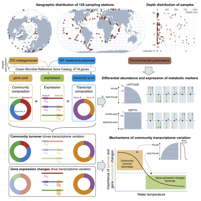
Graphical Abstract

Highlights

• •A catalog of 47 million genes was generated from 370 globally distributed metagenomes
• •Meta-omics data integration disentangled the mechanisms of changes in transcript pools
• •Transcript pool changes of metabolic marker genes show distinct mechanistic patterns
• •Community turnover as a response to ocean warming may be strongest in polar regions

A global survey of gene and transcript collections from ocean microbial communities reveals the differential role of organismal composition and gene expression in the adjustment of ocean microbial communities to environmental change.

Introduction

Microorganisms perform ecological functions and drive biogeochemical cycles that transform matter and energy on a global scale (Falkowski et al., 2008). Recent advances in sequencing technology and the analysis of DNA extracted from environmental samples (metagenomics) have made it possible to systematically characterize the taxonomic and genomic composition of microbial communities in diverse biomes (Fierer et al., 2012, Human Microbiome Project Consortium, 2012, Sunagawa et al., 2015). In the ocean, such biodiversity surveys have been conducted on local (Karl and Church, 2014, Venter et al., 2004), as well as regional and global scales (Biller et al., 2018, Kent et al., 2016, Rusch et al., 2007, Sunagawa et al., 2015). These and similar efforts (Delmont et al., 2018, Duarte, 2015, Kopf et al., 2015, Tully et al., 2018) have provided valuable baseline data that reveal the biodiversity of ocean microbial taxa, the repertoire of genes and genomes in the ocean, and the ecological factors that structure ocean microbial communities.

Despite the rich information that can be obtained about the gene-encoded functional potential in an environment, metagenomics alone cannot predict which, and in what amount, specific functions contribute to the molecular activity of microbial communities in situ, because genes may be variably expressed or not expressed at all. In contrast, metatranscriptomics enables the analysis of the pool of transcripts from genes that are actually expressed in an environmental sample (Helbling et al., 2012, Moran et al., 2013, Poretsky et al., 2005) and therefore provides a more accurate depiction of ecologically relevant processes that are occurring (e.g., in response to diurnal or other variations in environmental conditions) (Ottesen et al., 2014, Poretsky et al., 2009). In addition, the integration of metagenomic and metatranscriptomic data to quantify levels of gene expression, that is, the relative amount of expressed transcripts per gene, has revealed a number of important insights. For example, the ecological importance of photosynthesis, carbon fixation, and ammonium uptake has been highlighted in Prochlorococcus, which is abundant in oligotrophic waters of the tropical and subtropical ocean, because genes encoding these functions were among the most highly expressed genes in their genomes (Frias-Lopez et al., 2008). Picocyanobacteria, in general, have been found to contribute more to the community pool of transcripts than expected by abundances inferred from metagenomics, whereas the opposite has been shown for some heterotrophic bacteria, including those from the highly abundant SAR11 clade (Dupont et al., 2015, Frias-Lopez et al., 2008, Shi et al., 2011).

In contrast to studying differences between gene and transcript abundances within samples, understanding why a pool of community transcripts (metatranscriptome) changes from one sample to another has received much less attention. Notably, changes in metatranscriptomes can result from alterations in the relative abundance of organisms and their associated genes (community turnover) and/or by changes in the expression of genes encoded among the community members (Satinsky et al., 2014) (Figure S1). For microbial communities in the Amazon River Plume, it has been shown, for example, that higher transcript levels for some functions (e.g., acquisition of phosphorous) could be explained by increased gene abundances in free-living communities whereas for other functions (e.g., sulfur cycling, vitamin biosynthesis, and aromatic compound degradation) higher transcript levels were attributed to increased gene expression levels in particle-attached communities (Satinsky et al., 2014). However, global-scale biogeographic patterns of community turnover versus gene expression-driven changes in metatranscriptomes, and the ecological determinants of the relative contribution driving these two mechanisms, have not yet been studied for marine or any other environmental microbial communities.

Figure S1.

Transcript Abundance Profile as a Function of Community Composition and Gene Expression, Related to STAR Methods

Cartoon exemplifying how an initial community with a given expression profile may result insimilar transcript abundance profiles through two different mechanisms: (i) changes in the community composition (upper arrow), represented by three different species (green, red, and blue), or (ii) changes in gene expression (lower arrow), represented by two different genes (purple and orange, with low and high expression levels, respectively).

Here, in order to better understand the basis of metatranscriptomic differences across environmental gradients (e.g., latitude and depth) in the ocean, we leveraged efforts from the Tara Oceans (2009–2013) expeditions (Karsenti et al., 2011) and analyzed an environmentally contextualized dataset (Pesant et al., 2015) of metatranscriptomes and metagenomes, which includes a circumpolar representation of the climate change-impacted Arctic Ocean (Hoegh-Guldberg and Bruno, 2010, Overland et al., 2018). To capture the abundances of genes and transcripts from ocean microbial communities at the species level, we established a reference catalog of non-redundant protein-coding sequences (hereafter, genes). Using this integrated information, we determined for a number of biogeochemical processes involved in photosynthesis, as well as in the cycling of carbon, nitrogen, and sulfur, varying contributions of community turnover, and gene expression changes to metatranscriptome differences across latitude and depth. We further compared, as a function of temperature, the relative contributions of these mechanisms and hypothesize how they will differ between polar and non-polar regions in response to ocean warming.

Results and Discussion

A New Meta-omics Resource for Global Ocean Microbiome Research

The dataset for this study consists of metatranscriptomic (n = 187) and metagenomic (n = 370) samples collected at 126 globally distributed sampling stations across a latitudinal range of 142° (Figure 1; https://doi.org/10.5281/zenodo.3473199). The samples originate from the light-penetrated, epipelagic waters from the surface (SRF), deep chlorophyll maximum (DCM), and mixed water layer, and dark waters from the mesopelagic (MES) layer, from 5 m to 1,000 m in depth (median depths of 5 m, 50 m, and 550 m for SRF, DCM, and MES, respectively). The 187 prokaryote-enriched metatranscriptomic libraries were generated and sequenced to an average depth of 28 Gbp per sample (https://doi.org/10.5281/zenodo.3473199), after protocol optimization for low-input RNA samples (Alberti et al., 2014) (STAR Methods). These data were analyzed in conjunction with a set of 131 virus-, 59 giant virus-, and 180 prokaryote-enriched metagenomes (https://doi.org/10.5281/zenodo.3473199), which include prior sequencing efforts of Tara Oceans (Sunagawa et al., 2015), virus-enriched metagenomes from polar (n = 44) and non-polar (n = 42) regions (Gregory et al., 2019, Roux et al., 2016) (see STAR Methods for definitions), and 41 prokaryote-enriched metagenomes from the Arctic Ocean (new to this study).

Figure 1.

Geographic Coverage of the Meta-omics Dataset Analyzed in This Study

Geographic distribution of the sampling stations of the Tara Oceans (2009–2013) expeditions (Pesant et al., 2015). Several size-fractionated samples were collected from different depth layers at each station for a total of 557 samples (370 metagenomes and 187 metatranscriptomes). Stations numbered 155 and above represent the Tara Oceans Polar Circle campaign undertaken between June and October 2013. Colors indicate the type of samples collected for the prokaryote-enriched fractions at each station: metagenome only (orange, 18 stations); metatranscriptome only (blue, 40 stations); metagenome and metatranscriptome for at least one of the depth layers (green, 68 stations).

We aimed to capture whole community-level variations in community turnover and gene expression changes and to place these data into the context of geographic and environmental gradients at a global scale. Notably, the applicability of this approach critically depends on the evolutionary distances between the organisms present in the environment and those represented in genomic sequence databases (Nayfach et al., 2016). Ideally, genome sequences would be available for all organisms that comprise the communities of interest, thus facilitating the integration of gene abundance and gene expression data to assess whole-community compositions. Such analyses appear to be within reach for the human gut microbiome, for which appropriate genomic resources have recently become available (Almeida et al., 2019, Nayfach et al., 2019, Pasolli et al., 2019). However, for ocean microbiome samples, less than 10% of metatranscriptomic, and less than 5% of metagenomic data, can currently be resolved at the species-level using available marine genomic sequence databases (Figure 2A).

Figure 2.

Gene Detection Rates and Annotation of the OM-RGC.v2

(A) Percentage of reads from 180 prokaryote-enriched metagenomes (orange) and 187 prokaryote-enriched metatranscriptomes (blue) aligned with a 95% identity cutoff to: the MarRef database v3, updated 2019/01/19 (Klemetsen et al., 2018), a collection of metagenome-assembled genomes (MAGs) reconstructed from Tara Oceans samples (Delmont et al., 2018), and the OM-RGC.v2 (this study). To fairly compare the alignments to the MarRef database or MAGs and the catalog, we corrected for the gene coding density in prokaryotic genomes (STAR Methods). Boxplots show the median values as horizontal lines, interquartile ranges as boxes with whiskers that extend up to 1.5 times the interquartile range, and outliers as individual data points.

(B) The accumulation of OM-RGC.v2 genes detected in 180 prokaryote-enriched samples. The dashed line separates the prokaryote-enriched non-Arctic metagenomes (n = 139) (Sunagawa et al., 2015) from the Arctic metagenomes (n = 41). The increase in slope reflects an increase in the rate of detection of new genes in the Arctic Ocean. The non-prokaryote-enriched metagenomes (n = 190) and the metatranscriptomes (n = 187) are excluded from this analysis.

(C) The taxonomic annotation of genes at the domain level (and viruses; LUCA, last universal common ancestor) and the breakdown of gene functional annotations into ∼9 k KEGG and ∼76 k eggNOG orthologous groups (KOs and OGs, respectively). The remaining fraction of unannotated genes was used to generate de novo gene clusters (GCs) for further functional characterization of the catalog.

To overcome this limitation, we generated an updated version of the Ocean Microbial Reference Gene Catalog (OM-RGC.v2; original version in Sunagawa et al., 2015) based on 370 metagenomes with extended geographic coverage, particularly for the Arctic Ocean (Figure 1). Among the 47 million non-redundant genes, 24.5% were reconstructed, although partially detected elsewhere (Figure 2), in the Arctic Ocean samples alone, highlighting the added value of sampling genomically underexplored environments. Using this reference, nearly 70% of the genes could be taxonomically annotated, and 61% showed homology to known (i.e., existing) orthologous groups (OGs) in the database used for gene functional annotation (eggNOG version 4.5) (Huerta-Cepas et al., 2016) (STAR Methods). We further grouped the remaining 39% of the genes in the OM-RGC.v2 that represent unknown genes (i.e., genes of unknown function without detectable homology to known sequences), into ∼250,000 gene clusters (GCs) based on shared sequence similarity (Figure 2C; STAR Methods). We identified significant differences when comparing transcript abundances between depth layers (for 5,439 GCs) or between polar and non-polar regions (for 31,339 GCs), or correlations with environmental parameters (for 21,648 GCs) (Figure S2). These findings suggest ecologically relevant yet unknown functions of these genes in response to environmental variation. A benchmarked analysis of conserved co-expression as a method for identifying functionally related genes (Stuart et al., 2003) suggests that some of the GCs are likely to represent unidentified players in signal transduction, transcriptional regulation, and energy production/conversion (Figure S3; Table S1).

Figure S2.

Prevalence and Statistical Associations to the Environment of OGs and GCs, Related to STAR Methods

Gene abundance-based prevalence versus transcript abundance-based prevalence (i.e., number of samples in which detected) for (A) eggNOG-based orthologous groups (OGs) and (B) de novo gene clusters (GCs) based on the 122 paired metagenomes and metatranscriptomes. Prevalence distributions are shown in the side and upper panels. The numbers of OGs and GCs with significant associations of transcript abundances to depth layers (C) and polar/non-polar regions and (D) to environmental variables are shown. Associations were detected as statistically significant differences in transcript abundance by Wilcoxon tests for depth layers and polar/non-polar regions (p < 0.05, after Holm correction for multiple comparisons) and as significant Pearson correlations for environmental variables (|r| > 0.6 and p < 0.05, after Holm correction for multiple comparisons). In both cases only the OGs and GCs with a transcript abundance-based prevalence higher than 10% were considered in order to avoid spurious associations.

Figure S3.

Rationale for the Use of Co-expression Data to Associate Groups with Unknown Functions to Known Functional Groups, Related to STAR Methods

Evaluation of model performance for the link between OGs based on co-variation analysis. (A) Receiver operating characteristic (ROC) curves for all models. Variation in (B) false positive rate and (C) sensitivity with increasing Pearson correlation values used as a cut-off for classification (r_min). The r_min is a value to be optimized corresponding to the minimum Pearson r that provides sufficient predictive power (false positive rate < 5%). A total of nine models are represented, which used co-abundance, co-transcription, and co-expression for the prediction of shared KEGG reactions, modules, and pathways, respectively, between pairs of OGs (see details in STAR Methods).

In contrast to existing ocean genomic reference databases, we found the OM-RGC.v2 to capture the majority of gene-encoding metagenomic and metatranscriptomic data (70% and 51%, respectively) (Figure 2A) used in this study, making it a suitable resource to address our aim of analyzing whole-community metatranscriptomic compositions. All gene sequences can be queried online for their abundance, expression, and geographic distribution (Villar et al., 2018), and they are linked to contextual environmental parameters (Pesant et al., 2015) facilitating additional gene-centric explorations in the future.

Variation of Meta-omic Compositions across Latitude and Depth

Having established resources to quantify whole-community taxonomic, genomic, and transcriptomic compositions, we next sought to identify patterns and drivers of compositional structure across major axes of environmental variation in the ocean biome at a global scale. Numerous studies have revealed that microbial communities are vertically stratified in the ocean, with a striking boundary between epipelagic and mesopelagic zones (DeLong et al., 2006, Giovannoni and Stingl, 2005, Sunagawa et al., 2015). Polar and non-polar communities have also been shown to separate into distinct groups with different species-level taxonomic compositions (Ghiglione et al., 2012, Gregory et al., 2019). Critically, however, the shared gene content between different strains of the same species may be as low as 40%, as has been shown, for example, in Escherichia coli (Mira et al., 2010). Furthermore, gene functional redundancy in microbial communities (i.e., when the same gene functions are encoded by different taxa) may help to maintain important community functions in cases of biodiversity loss (Bell et al., 2005). Thus, it is difficult to predict whether gene functional compositions and gene expression-regulated transcriptomic repertoires would follow the same patterns of taxonomic composition changes.

To address this question, we first aimed to locate the boundaries of differentiation (Ludwig and Cornelius, 1987) in epipelagic waters (SRF and DCM) along the latitudinal gradient for different community-compositional measures derived from the prokaryote-enriched metatranscriptomes and metagenomes (STAR Methods). From the equator northward, no significant differentiation was identified in epipelagic waters until a latitude of 40°N. At this point, the degree of differentiation increased significantly for all community-compositional measures and peaked at around 60°N. A similar trend was also observed for the southern hemisphere (Figure 3) and is consistent with the taxonomic compositional differences observed between polar and non-polar waters for bacterial (Ghiglione et al., 2012, Gregory et al., 2019) and viral communities (Ghiglione et al., 2012, Gregory et al., 2019). We further found that the differentiation is reflected by significant enrichments of operational taxonomic units (OTUs) from the order Flavobacteriales (e.g., Formosa, Polaribacter, NS5, NS7, and NS9 marine groups), the class Gammaproteobacteria (OM182 clade and Piscirickettsiaceae), and eukaryotes (e.g., Phaeocystis), as well as by depletions of Prochlorococcus spp., members of the Rhodospirillaceae family, and members of the SAR11 and SAR406 clades toward higher latitudes (Figure S4). Here, the congruent patterns observed for both metagenomic and metatranscriptomic differentiation—measured as changes in the relative abundance of gene and transcript copies at the level of OGs—indicate that on a global scale, taxonomic composition largely shapes the composition of gene functional content. Organismal composition also dominates over gene regulatory variations in shaping community-level transcriptomic compositions across ecological boundaries.

Figure 3.

Latitudinal Partitioning of Global Ocean Microbiome Compositions

The schematic on the left illustrates the underlying concept of the split moving-window analysis of ecological differentiation (Ludwig and Cornelius, 1987). It consists of a comparison of the pairwise distances between communities on opposite sides of a putative boundary with the pairwise distances between communities on the same side. A high differentiation value captures an increase in the distance between the two sides of the boundary compared with the distances within each side. The analysis was conducted with a window width of 10 samples and shows an ecological boundary centered around 60°N based on the taxonomic composition (gray, relative abundance of OTUs), metagenomic composition (orange, per-cell abundance of genes), and metatranscriptomic composition (blue, relative per-cell abundance of transcripts) of prokaryote-enriched samples from surface (SRF) and deep chlorophyll maximum (DCM) waters (both belonging to the epipelagic layer). A similar pattern is evident for the southern hemisphere; however, the limited number of samples precluded detection of an ecological boundary. Significance was determined using 99% confidence intervals computed with 10,000 random permutations of the latitude values. Vertical lines represent the window of the latitudinal range of significant values. The insufficient number of samples and latitudinal coverage prevented us to perform this analysis for the mesopelagic layer.

See also Figure S4.

Figure S4.

Differential Abundance of the Dominant OTUs along the Latitudinal Gradient, Related to Figure 3

Latitudinal niche value (i.e., the abundance-weighted mean absolute latitude) for the 60 most abundant OTUs in the epipelagic subset of samples. Latitudinal niche values significantly higher and lower than the value expected from a random distribution of abundances (represented by the horizontal bold lines; see STAR Methods) are color coded. The dot size is proportional to the mean relative abundance of each OTU.

Indeed, we found that all community-compositional measures were highly correlated (Figure S5), and their variability in the epipelagic ocean was, among a set of 27 environmental parameters, best explained by seawater temperature (Figure 4A). This result complements earlier reports of temperature as an important factor driving the taxonomic composition of ocean microbial communities (Fuhrman et al., 2006), which was corroborated by a later analysis of a globally distributed set of samples that accounted for geographic effects and disentangled temperature from other environmental parameters to confirm that it acts as a key driver of taxonomic and gene functional compositions in epipelagic, non-polar open ocean waters (Sunagawa et al., 2015). In fact, the identification of an ecological boundary starting at 40°N and peaking at 60°N coincides with a steep temperature decrease between the North Atlantic and Arctic waters that were sampled (Figure S6) and relates to additional oceanographic features. At ∼40°N/S, the 15°C annual-mean isotherm effectively delineates the permanently stratified ocean from the subpolar and polar regions (Behrenfeld et al., 2006), while winter mixing in the North Atlantic is the strongest (deepest mixed layer depth) at ∼60°N (Montégut et al., 2004). The ecological boundary we describe here for microbial community compositions could thus be due to physico-chemical changes driven by the variability in the vertical mixing of oceanic water masses, which is linked to differences in sea surface temperature.

Figure S5.

Correlations between the Taxonomic, Metagenomic, and Metatranscriptomic Composition, Related to Figure 4

All pairwise correlations between the Euclidean distance of the (log₂-transformed) taxonomic, metagenomic, and metatranscriptomic profiles were computed for 122 samples for which all three profiles were available. The correlation strength and significance were assessed using Mantel tests with 10,000 permutations.

Figure 4.

Patterns and Drivers of Global Ocean Microbiome Compositions across Depth Layers and between Polar and Non-polar Regions

(A) Taxonomic, metagenomic, and metatranscriptomic composition of epipelagic samples (based on _mitags, and the normalized abundances of eggNOG-derived OGs from metagenomic and metatranscriptomic data, respectively) were related to each of 27 environmental factors using partial (geographic distance-corrected) Mantel tests with 10,000 permutations and Bonferroni correction. Pairwise comparisons of environmental factors are shown below, with a color gradient denoting Spearman’s correlation coefficients. Temperature is the best explanatory variable for all of the profiles in the epipelagic ocean (taxonomic profile: Pearson’s r = 0.75; metagenomic profile: Pearson’s r = 0.69; metatranscriptomic profile: Pearson’s r = 0.64; all p < 0.05), followed by oxygen concentration, which is highly correlated to temperature (Pearson’s r = −0.72). A more detailed description of the variables is available in https://doi.org/10.5281/zenodo.3473199.

(B) Compositional richness of polar and non-polar microbiomes across three depth layers. Taxonomic and functional metagenomic richness (numbers of OTUs and OGs, respectively) increases with depth, although the richness is consistently lower in polar samples than in non-polar samples (two-way ANOVA: p < 0.05 for depth layers and polar/non-polar, for both taxonomic and metagenomic functional richness). By contrast, there was no significant difference in functional metatranscriptomic richness (number of OGs), either across depths or between polar and non-polar samples (two-way ANOVA: p > 0.05 for depth layers and polar/non-polar). Violin plots represent the (mirrored) density distribution of the data with the median shown as a horizontal line.

(C) Correlations among species richness (number of OTUs), functional metagenomic (metaG) richness and metatranscriptomic (metaT) richness (number of OGs). Data were rarefied before richness computation (STAR Methods). Pearson’s correlation was used for all comparisons (OTU-metaG; r = 0.78, p < 0.001; OTU-metaT: r = 0.16, p = 0.06; metaG-metaT: r = 0.39, p < 0.05). The solid line corresponds to the best linear fit. N.S., not significant (p > 0.05).

See also Figures S5 and S6.

Figure S6.

Latitudinal Distribution of Seawater Temperature in the Epipelagic, Related to Figure 4

Seawater temperature (°C) measurements (n = 528) at the surface (SRF) and the deep chlorophyll maximum (DCM) along the Tara Oceans course in relation to (A) raw latitude values and (B) bins of the absolute latitude. Data are available at https://doi.org/10.1594/PANGAEA.875576.

We next quantified metatranscriptomic richness (i.e., the unique number of OGs detected by cDNA sequencing), as a proxy for the diversity of transcribed gene functions, and compared this to taxonomic and metagenomic richness (i.e., the unique number of detected OTUs and OGs, respectively, detected by DNA sequencing). As measures of diversity, the latter two provide information about the stability (McCann, 2000), functionality (Cardinale et al., 2006), and possibly productivity (Tilman, 1995, Vallina et al., 2014) of ecological communities. In addition, we sought to quantify the fraction of the gene-encoded functional potential in a given community that is actually transcribed at a given time by comparing metatranscriptomic and metagenomic richness.

Taxonomic and metagenomic richness were highly correlated, without showing signs of saturation, supporting the previous observation that functional redundancy in the marine ecosystem is rather low (Fierer et al., 2013, Galand et al., 2018), and both were found to be significantly lower in polar than in non-polar communities at all tested depth layers (Figure 4B). These data are congruent with studies suggesting a decrease in the taxonomic diversity of communities with increasing latitude (Fuhrman et al., 2008, Gregory et al., 2019, Ibarbalz et al., 2019, Sul et al., 2013) and an associated decrease in gene functional diversity, although other studies have also proposed alternative patterns of latitudinal diversity gradients (Ghiglione et al., 2012, Ladau et al., 2013, Raes et al., 2018). In contrast, metatranscriptomic richness was not correlated with taxonomic richness and only poorly correlated with metagenomic richness, and no significant difference was found between polar and non-polar microbiomes or between any depth layers (Figure 4B). This unexpected disparity between metagenomic and metatranscriptomic richness patterns suggests that the non-transcribed proportion of a given metagenome is higher in mesopelagic waters and non-polar regions relative to epipelagic waters and polar regions. This could be due to a higher proportion of dormant or dead, and passively sinking, microbes in the mesopelagic compared to the epipelagic ocean. Alternatively, these observations may reflect the prevalence of genome streamlining in surface ocean waters (Swan et al., 2013), where per genome, the number of genes is expected to be lower (Mende et al., 2017). The proportion of transcribed genes is thus expected to be higher than in mesopelagic waters. Future studies will be required to determine whether the apparent saturation of simultaneously transcribed gene functions, despite increasing numbers of encoded gene functions, is a feature that is also common in microbial communities from other biomes.

Differential Abundance and Expression of Biogeochemical Cycling Genes

The pool of microbial community transcripts may vary along environmental gradients as a function of community turnover and/or changes in gene expression (Figures S1 and S7; STAR Methods). To disentangle the individual contributions of these mechanisms across environmental gradients for genes that are involved in ecologically relevant processes, we integrated 122 prokaryote-enriched, matched metatranscriptomes and metagenomes and quantified the differential abundances and expression levels for a set of biogeochemical marker genes across depth layers and between polar and non-polar waters (Figure 5).

Figure S7.

Derivation of the Decomposition of a Metatranscriptome, Related to STAR Methods

Mathematical basis for (A and B) the within-sample decomposition of metatranscriptomes (transcript copies / cell) into abundance (gene copies / cell) and expression (transcript copies / gene copy) components, and for (C) the between-sample decomposition of the Euclidean distance between metatranscriptomes (transcript abundance differences) into the abundance component (gene abundance differences), the expression component (expression differences), and an interaction term (abundance - expression covariation). See details in STAR Methods.

Figure 5.

Differences in Gene Abundance and Expression Determine Differential Transcript Abundances of Metabolic Marker Genes across Depth Layers and between Polar and Non-polar Regions

(A and B) Differences in the abundance of genes and transcripts, and the gene expression level of metabolic marker genes (KOs) were determined (A) between epipelagic and mesopelagic layers and (B) between polar and non-polar regions. The data points show the differences in the mean transcript abundances, mean gene abundances, and mean gene expression (i.e., transcript abundance normalized by gene abundance) of KOs. Differences were computed using log₂-transformed values (STAR Methods) and tested for significance by Mann-Whitney tests. Differences were considered significant if p values after Holm correction were smaller than 0.05. Only epipelagic samples were used for the data shown in (B).

See also Figures S8, S9, S10, and S11.

As a first step, we sought to validate both data quality and our analytical approach by testing whether patterns for genes involved in well-studied processes, including carbon fixation, photosynthesis, and nitrogen cycling could be observed. As expected, we found that the most differentially abundant transcripts between epipelagic and mesopelagic layers included those from the photosynthesis marker genes, psaA and psbA, and genes encoding the subunits of RuBisCO (rbcL and rbcS), the key enzyme required for carbon fixation (Figure 5A). Moreover, we observed that abundances of the rbcL and rbcS transcripts were highly correlated with those of psaA and psbB, which is consistent with the expectation that carbon fixation is primarily driven by photoautotrophs rather than chemoautotrophs (Raven, 2009, Shively et al., 1998, Swan et al., 2011). This is further supported by the observation of low RuBisCO gene expression levels in mesopelagic waters, despite the presence of chemoautotrophs (Figure S8). In addition to psbA, the abundances of other photosynthetic marker genes, including markers for the photosynthetic reaction center (petC, petE, and petH) and the cyanobacteria-specific antenna proteins (apcA, apcF, cpcA, cpeA, and cpeT), were lower in polar than in non-polar waters (Figure 5B). This result likely reflects the depletion of cyanobacteria in colder environments (Marchant et al., 1987) (Figure S4) and an underrepresentation of eukaryotic phototrophs in the prokaryote-enriched samples we analyzed here.

Figure S8.

Gene and Transcript Abundance of RuBisCO Subunits and PSI and PSII Marker Genes, Related to Figure 5

Distribution of whole-community (log₂-transformed) (A) gene and (B) transcript abundances of the RuBisCO subunits (rbcS and rbcL) and the marker genes for photosystem I (psaA) and II (psbA) in the epipelagic and mesopelagic depth layers. Pairwise correlations based on the (C) gene and (D) transcript abundances of the four genes are shown below. All comparisons, except the ones denoted with N.S. in (A) and (B) were significant (p < 0.05 using Wilcoxon test and Holm correction for multiple comparisons). All Pearson correlations in (B) and (C) were significant (p < 0.05).

With respect to nitrogen cycling, we detected both gene and transcript abundances for denitrification marker genes (napA, nirS, norB, and nosZ) to be enriched in mesopelagic versus epipelagic waters (Figure 5A). As expected for this predominantly anaerobic process (Zehr and Ward, 2002), transcript abundances were particularly high in oxygen-depleted waters, although interestingly, similar transcript levels were also observed in some well-oxygenated Arctic water samples (Figure S9). Transcripts of nitrogen fixation marker genes (nifK, nifH, and nifD) were more abundant in non-polar than in polar regions, with the highest abundances detected in waters between 20° and 35° (absolute latitude) with low nitrate and nitrite concentrations (Figure S10). These data generally agree with the long-standing expectations that nitrogen fixation activity is higher under conditions of nitrogen limitation and is primarily driven by cyanobacteria in tropical and subtropical regions (Dixon and Kahn, 2004, Stal, 2009). However, more recent studies have provided additional evidence for an extended geographic and depth range (Blais et al., 2012, Harding et al., 2018, Moisander et al., 2017) and for a wider taxonomic breadth of nitrogen fixing organisms including non-cyanobacterial heterotrophic diazotrophs (Bombar et al., 2016, Delmont et al., 2018). Given these findings, we further investigated the biogeography of the nifH gene in more detail and determined which organisms not only encode this gene, but also express it. Specifically, we analyzed the distribution of nifH gene and transcript abundances among 24 nifH-encoding “species” that were detected in the 122 matched metagenomes and metatranscriptomes. From this analysis, we found that a number of Gamma- and Deltaproteobacteria, for which genomes have recently been reconstructed (Delmont et al., 2018), were not only abundant, but also among the top contributors to the nifH transcript pool in the studied samples (Figure 6). Additionally, for the first time, to our knowledge, we detected nifH gene expression in mesopelagic Arctic waters and reconstructed the nif operon-containing genome of its carrier (http://doi.org/10.5281/zenodo.3352180; STAR Methods), a candidate heterotrophic Deltaproteobacterium or a member of the Myxococcota phylum according to a recent proposal for a standardized bacterial taxonomy (Parks et al., 2018), that awaits further characterization.

Figure S9.

Transcript Abundance of Denitrification Marker Genes along the Oxygen Gradient, Related to Figure 5

The log_2-transformed transcript abundances of nirS, norZ, nosB, and napA in relation to the oxygen concentration at the sampling location, showing a high transcript abundance in samples taken from anoxic waters (< 100 μM) and interestingly, from oxygenated waters at stations 206, 208, and 210. The depth layer (EPI or MES) and polar/non-polar nature of the sample are coded as the symbol type and color, respectively. The dot size is proportional to the concentration of NO₂ and NO₃ (μM) when available.

Figure S10.

Expression and Transcript Abundance of the nifH, nifD, and nifK Genes in Relation to Nitrate and Nitrite Concentration, Related to Figure 5

Gene expression and transcript abundance of the nifH, nifD, and nifK genes in relation to the total nitrate plus nitrite concentration (μM), showing a fast decay of gene expression and transcript abundance with increased in nitrate/nitrite concentrations from 0 to 0.2 μM at absolute latitudes between 20° and 35°. Solid lines correspond to the result of local regression.

Figure 6.

Relative Gene and Transcript Abundance of 24 Nitrogenase Genes (nifH) Representing nifH-Encoding “Species”

(A–D) Relative gene (orange) and transcript (light blue) abundance distributions of the 24 nifH genes from the OM-RGC.v2 that were detected in 122 matched metagenomes and metatranscriptomes (A) are shown and broken down by latitude (B) and by depth (C) of the sample origin. Genes (IDs in the bottom panel) were annotated using a nifH-specific database (see STAR Methods). Boxplots in (A–C) show the median values as horizontal lines, interquartile ranges as boxes with whiskers extending up to 1.5 times the interquartile range, and all values overlaid as individual data points. Colors denote phylum-level taxonomic annotations, naming corresponds to finer grain taxonomy or database-specific identifiers (D), and stars indicate genes that were previously identified in MAGs of heterotrophic bacterial diazotrophs (HBDs) (Delmont et al., 2018). The genome containing a nifH gene for which transcripts were detected in the mesopelagic layer in the Arctic (OM-RGC.v2.019519152, bold) was reconstructed (see STAR Methods and http://doi.org/10.5281/zenodo.3352180). Horizontal dashed lines denote the latitude and depth that were used to define polar and non-polar (B) and epipelagic and mesopelagic waters (C), respectively.

In spite of the potential biases inherent to our approach that are related to the collection of spatially discrete data over a period of more than 3 years and to the sampling process itself (e.g., unaccounted effect of seasonality or potential changes in transcript abundances during the sampling process), we were able to corroborate expected patterns of metabolic processes using metatranscriptomic data at global scale. In addition to validating our methods, we demonstrated how our community-centric approach for analyzing metatranscriptomes can be used in conjunction with metagenomic data, and furthermore, bridge to new genome-resolved insights. Building on the robustness of our analysis, we next focused on disentangling the mechanisms that underpin the differences in community transcriptomes across depth and latitude. Notably, we observed cases in which transcript abundance changes could be mainly attributed either to differences in gene abundance or gene expression or a combination of these mechanisms. As described above, the enrichment of transcripts from denitrification marker genes in mesopelagic versus epipelagic waters are mainly driven by changes in gene abundance (Figure 5A). In this case, gene abundance changes, due to environmental filtering of organismal community composition in response to higher nitrate and nitrite concentrations in mesopelagic waters, dominate the observed community transcriptomic differences. Conversely, a higher transcript abundance of marker genes for anaerobic dissimilatory sulfate reduction (aprA and aprB) in epipelagic waters is driven by an increased expression of these genes, despite no significant differences in the abundance of these genes between depth layers (Figure 5A). A taxonomic breakdown shows that 39% and 59% of aprA and aprB genes were encoded by Proteobacteria, and only 2% of each gene could be assigned to taxa containing known sulfate reducers (Archaea, Firmicutes, Nitrospirae, and Deltaproteobacteria) (Muyzer and Stams, 2008). These results suggest that the significance of alternative uses for aprA and aprB in oxic waters, namely to detoxify cells by catalyzing the oxidation of sulfite accumulated in the cytoplasm, as described for clades such as SAR11 and SAR116 (Meyer and Kuever, 2007, Smith et al., 2016), may be of global relevance.

A more complex scenario for observing differences in transcript pools is exemplified by a number of marker genes for assimilatory sulfate reduction (cysD, cysH, cysI, cysJ, and cysN), for which the observed differences across the latitudinal gradient (i.e., higher transcript abundances in non-polar versus polar regions) result from a combination of community turnover and gene expression changes. In this case, the increased transcript abundance in non-polar waters results from higher expression levels, despite a lower abundance of genes. Interestingly, we found the transcript abundance of these marker genes to be anticorrelated with that of dmdA (Figure S11), the key gene for the demethylation of dimethylsulfoniopropionate (DMSP) (Howard et al., 2006), which results in incorporation of carbon and sulfur into bacterial biomass (Kiene et al., 1999). Based on these data, we hypothesize that the global-scale expression of the assimilatory sulfate reduction pathway may be downregulated in response to the availability of DMSP, which is used by prokaryotes as an alternative source for sulfur assimilation (Kiene et al., 2000). Notably, if turnover and differential gene expression are both operative, relying on gene abundance alone may lead to false predictions including patterns that would suggest the opposite of what is manifested at the transcript level (e.g., non-photosynthetic carbon pathways with higher epipelagic expression levels but higher mesopelagic gene abundances of mct and abfD).

Figure S11.

Correlation between Assimilatory Sulfate Reduction Marker Genes and the dmdA Gene, Related to Figure 5

Transcript abundance and expression of the genes involved in the assimilatory sulfate reduction pathway in relation to the transcript abundance of the dmdA gene involved in the dimethylsulfoniopropionate (DMSP) demethylation pathway. Pearson correlation was used to test for significance of the correlation. Pearson r values and significance are shown on the plot. Log₂-transformed data were used in all cases. The correlation with the transcript abundance was significant for all genes and was especially high (−0.73) for cysD and cysN, the genes encoding the initial step of the pathway (i.e., the reduction of sulfate).

Turnover Dominates over Gene Expression Differences in Polar Water Communities

In light of global climate change, a better understanding of how ocean microbial communities will respond to ongoing changes is urgently needed (Cavicchioli et al., 2019, Overland et al., 2018). In particular, the Arctic region has experienced some of the highest ocean surface water temperature anomalies recorded to date (Hoegh-Guldberg and Bruno, 2010). Ocean warming models (scenario RCP 8.5, business as usual) predict that mean surface water temperatures will increase by 2°C to 5°C in the Arctic by the end of the century (Alexander et al., 2018), highlighting a critical need to better understand how these changes will impact microbial communities in this region. Given that these projections focus on surface temperature changes and due to their major contribution to biogeochemical cycles (Field et al., 1998), we sought to assess the response of epipelagic communities to environmental variation, as reflected by measurable differences in their metatranscriptomic composition, and subsequently to use these spatially discrete data to hypothesize on future projections.

Specifically, we aimed to disentangle (Figure S7; STAR Methods) whether differences in microbial community transcriptomes are impacted more strongly by community turnover and/or by gene expression changes along the temperature gradient at their sampling locations. To this end, we divided all samples into groups of 15 samples (bins) using a sliding window along the temperature gradient, so that each group reflected the range of ocean warming expected before the end of the century (median temperature difference within each bin: 1.6°C; Figure S12A). We then quantified the different mechanisms of metatranscriptome changes within each bin (Figure 7; STAR Methods) and found that in warmer epipelagic waters, the relative contribution of community turnover to metatranscriptomic compositional dissimilarities is significantly lower than that of gene expression changes. In contrast, the effect of community turnover in colder (predominantly Arctic) waters is higher or in the same range as gene expression changes (Figure 7A). Overall, community turnover was found to be significantly higher in polar communities than in non-polar communities (p < 0.001), whereas gene expression changes displayed the opposite pattern (p < 0.001) (Figure 7B). Interestingly, the shift in the relative contributions of the different mechanisms of metatranscriptome changes occurs at ∼15°C and therefore coincides with the ecological boundary previously identified, which, as such, not only delineates communities differing in their composition but also in the mechanism shaping their transcript pool. We further found that the effect of temperature was greater than that of other environmental variables, such as nitrate/nitrite concentrations and salinity (Figure S12), suggesting a higher acclimatory capacity of microbial communities in warm than in cold epipelagic waters in response to temperature variations.

Figure S12.

Temperature Dominates over Other Environmental Variables in Structuring the Relative Contribution of Community Turnover and Gene Expression Changes to Metatranscriptomic Differences between Epipelagic Communities, Related to Figure 7

Panel (A) mirrors the data in Figure 7A, so that it represents the groups of 15 samples (bins) along the temperature gradient on the x axis. The y axis, however, captures the distribution of the temperature differences within each bin. Notably, the distributions of these differences are highly similar in polar and non-polar waters. This indicates that the higher relative contribution of turnover in polar waters and gene expression changes in non-polar waters occurs for a similar range of temperature differences. (B) The distribution of the interaction component (see Equation 1 in STAR Methods) for all the polar-to-polar and non-polar-to-non-polar comparisons across the bins are not significantly different from each other (Wilcoxon test), which indicates that the absolute values of turnover and gene expression changes are comparable between polar and non-polar communities (Figure 7B). Panel (C) is based on Figure 7A and serves as an explanatory schematic for panel (D). To evaluate the influence of an environmental parameter on the relative contribution of community turnover and gene expression changes, a similar analysis to the one in Figure 7A was performed. A score was attributed to each parameter as the sum of the deviation of each bin from 1 (where the effect of both mechanisms is identical). The deviation of each individual bin is visualized as a gray line. The results are summarized in panel (D) for the environmental parameters that were tested. The vertical lines indicate the distribution of this score for 100 random binnings (solid line denotes the median value and dashed lines represent the 95% interval of the distribution). As a result, we identify that daylength, temperature and chlorophyll concentrations have significant effects on the relative contributions. We further investigated these parameters, by assessing the distribution of environmental variation for polar and non-polar regions across the bins [panels (E), (G), and (I)], and the relationship between the relative contributions (of community turnover and gene expression changes) and the variation in the environmental parameter across the whole (unbinned) dataset [panels (F), (H), and (J)]. The left-side [(E), (G), and (I)] aims at answering whether the difference in regimes that are observed between polar and non-polar regions may simply be due to a different range of environmental variation. The distributions display little differences in the case of temperature, while they are strongly contrasted for daylength and chlorophyll concentrations. Furthermore, (F), (H), and (J) provide a direct estimation of the relationship of the relative contributions of community turnover and gene expression changes with the environmental distance. Based on linear models, temperature differences capture most of the variance, both in polar and non-polar regions. In contrast, daylength and chlorophyll concentrations show a weaker or no trend, especially in polar regions (despite a wide range of variation). Overall, this confirms that among the parameters tested, temperature is the best explanatory variable for the difference in the relative contribution of community turnover and gene expression changes observed between polar and non-polar epipelagic communities.

Figure 7.

Relative Contributions of Community Turnover and Gene Expression Changes to Variations in Metatranscriptome Composition

Determination of the relative contributions of community turnover and gene expression changes to variations in the metatranscriptome composition requires the decomposition of metatranscriptomic distances between communities (Figure S7; STAR Methods). Specifically, the relative contribution is determined as the ratio of the gene abundance-based distance (community turnover) and the gene expression-based distance (gene expression changes) between two metatranscriptomes.

(A) The relationship of the ratio with temperature was analyzed by dividing the epipelagic samples into groups (bins) of 15 samples each using a sliding window along the temperature gradient. For each bin, we report the median ratio (among all the pairwise comparisons within each bin) as a function of the median temperature of the samples present in the bin. The significance is determined by a Wilcoxon test comparing the within-bin distribution of the ratios to 1 (in which case the relative contributions of community turnover and gene expression changes are the same). The Holm correction was used to adjust for multiple testing. The ratio was considered to be significantly different from 1 if p < 0.05.

(B) The inner panel represents the difference for community turnover and gene expression changes between polar and non-polar regions. The distributions capture the distances of each component for all pairwise comparisons of polar and non-polar epipelagic samples. Violin plots represent the (mirrored) density distribution of the data with the median shown as horizontal line. Significance was tested by the Wilcoxon test; ^∗∗∗p < 0.001.

See also Figure S12.

Finally, by extrapolating our results from spatially discrete data to potential consequences of climate change (Blois et al., 2013), we hypothesize that the relative impact of organismal composition changes on microbial community transcriptomes will be greater in polar than in non-polar waters. This extrapolation, however, needs to be interpreted within the limitations of the data analyzed here, namely that it cannot account for the evolutionary adaptation of microbial communities to gradual changes with time. As such, further studies resolving long-term temporal dynamics of metatranscriptome changes are required to improve our understanding of the contributions of community turnover and gene expression changes in the context of environmental changes. Notwithstanding, the present results provide a first global-scale evaluation of the mechanisms underpinning the changes in community transcriptomes as well as a framework for future work.

Conclusions

Large-scale oceanographic sampling expeditions, such as the World Ocean Circulation Experiment (WOCE) or GEOTRACES (Anderson et al., 2014, Koltermann et al., 2011, Woods, 1985) have been extremely valuable in building our understanding of the ocean circulation, and the distribution of major nutrients and elements including trace metals, as well as their contribution to the climate system. However, our geochemical and physical knowledge of the ocean remains incomplete without incorporating the processes that regulate biogeochemical cycles at planetary scale (Falkowski et al., 2008). Analyzing the repertoire of genes and transcripts from environmental samples can inform us about the potential and activity of microbial communities that drive these cycles at global scale and thus help us to understand the intertwined processes that shape the physico-chemical state of the ocean through biological activity.

In this study, we describe global biogeographical patterns of microbial community transcriptome compositions and demonstrate how changes in these compositions can be attributed to community turnover and/or gene expression changes as the underlying mechanisms. Assessing the mechanisms that underlie such compositional differences, as demonstrated here, can help us to determine whether changes in the molecular activities of microbial communities are regulated by gene expression changes or by a turnover of organisms containing genomic modifications that arose over evolutionary time. In addition, an improved understanding of the ecological factors that drive community compositional and diversity changes can help us to better predict how ocean microbial communities will respond to environmental changes. For example, the consistent identification of temperature as a major explanatory factor for global-scale community-level differences in genomic (Sunagawa et al., 2015) and transcriptomic (this study) composition, as well as taxonomic diversity (Gregory et al., 2019, Ibarbalz et al., 2019), has wide-ranging implications, in particular for the Arctic Ocean, given the current projections of disproportionately high warming rates in this region (Alexander et al., 2018, IPCC, 2014).

Notably, the analyses of this study were enabled by a systematic, highly contextualized, pan-oceanic set of metagenomic and metatranscriptomic data that, along with the OM-RGC.v2, complements other large-scale datasets that have been developed for eukaryotes (Carradec et al., 2018, Ibarbalz et al., 2019), prokaryotes (Biller et al., 2018), and viruses (Gregory et al., 2019). Together, these will pave the way for an eco-systems level understanding of ocean plankton diversity, function, and activity across boundaries of organismal size ranges. To reach this goal, it will be important to integrate temporal meta-omics data, ideally from global observations, to account for seasonal variations and other concomitant environmental changes, such as increased stratification, acidification, nutrient availability, and deoxygenation of the oceans (Bopp et al., 2013, Schmittner et al., 2008). Such concerted efforts are required to further refine gene-to-ecosystem models (Coles et al., 2017, Garza et al., 2018, Guidi et al., 2016) and to inform environmental and climate policies (Le Quéré et al., 2018), which must consider not only how microorganisms are impacted by but also how they may affect anthropogenic climate change (Cavicchioli et al., 2019).

STAR★Methods

Key Resources Table

REAGENT OR RESOURCE	SOURCE	IDENTIFIER(S)
Sequencing Reagents and Kits
Ribo-Zero Magnetic Kit for Bacteria	Epicentre	MRZB12424
RNA Clean and Concentrator-5 kit	ZymoResearch	R1013
SMARTer Stranded RNA-Seq Kit	Clontech	634839
NEBNext Sample Reagent Set	New England Biolabs	E6000
Ampure XP	Beckmann Coulter	A63882
Platinum Pfx DNA polymerase	Invitrogen	11708039
SeqAmp DNA polymerase	Clontech	638509
Agilent 2100 Bioanalyzer	Agilent Technologies, USA	G2939BA
qPCR	MxPro, Agilent Technologies, USA	Mx3005P
Deposited Data
Tara Oceans metagenomes	Sunagawa et al., 2015, Roux et al., 2016; This paper	European Nucleotide Archive (https://www.ebi.ac.uk/ena) - see https://doi.org/10.5281/zenodo.3473199 for details
Tara Oceans metatranscriptomes	This paper	European Nucleotide Archive (https://www.ebi.ac.uk/ena) - see https://doi.org/10.5281/zenodo.3473199 for details
OM-RGC.v2 (catalog including assemblies and predicted genes), gene profiles, functional profiles, and taxonomic profiles	This paper	European Nucleotide Archive (https://www.ebi.ac.uk/biostudies/studies/S-BSST297) - see https://doi.org/10.5281/zenodo.3473199 for details
Environmental data	This paper	see https://doi.org/10.5281/zenodo.3473199 for details
MAG of putative nitrogen-fixing bacterium	This paper	https://doi.org/10.5281/zenodo.3352180
Software and Algorithms
MOCAT v2	Kultima et al., 2016	https://mocat.embl.de; RRID: SCR_011943
CD-HIT v4.6	Fu et al., 2012	http://cd-hit.org; RRID: SCR_007105
MMSEQS2	Steinegger and Söding, 2017	https://github.com/soedinglab/MMseqs2
megahit v1.1.2	Li et al., 2016	https://github.com/voutcn/megahit/releases/tag/v1.1.2
bowtie v2.3.2	Langmead and Salzberg, 2012	http://bowtie-bio.sourceforge.net/bowtie2/index.shtml; RRID: SCR_005476
BlastKOALA	Kanehisa et al., 2016	http://www.kegg.jp/blastkoala
eggNOG-mapper	Huerta-Cepas et al., 2017	https://github.com/jhcepas/eggnog-mapper/releases; RRID: SCR_002456
USEARCH v9.2.64	Edgar, 2010	https://www.drive5.com/usearch/download.html
metaBAT2 v2.12.1	Kang et al., 2019	https://bitbucket.org/berkeleylab/metabat/src/master/
CAP3 v021015	Huang and Madan, 1999	http://seq.cs.iastate.edu/cap3.html; RRID: SCR_007250
Geneious R10	N/A	https://www.geneious.com/; RRID: SCR_010519
CheckM v1.0.8	Parks et al., 2015	https://github.com/Ecogenomics/CheckM/releases/tag/v1.0.8; RRID: SCR_016646
GTDB-Tk v0.3.0	Parks et al., 2018	https://github.com/Ecogenomics/GTDBTk/releases/tag/0.3.0
Prokka v1.13	Seemann, 2014	http://www.vicbioinformatics.com/software.prokka.shtml; RRID: SCR_014732
R v.3.5.1	R Core Team, 2018	https://www.r-project.org; RRID: SCR_001905
R package vegan	Dixon, 2003	https://cran.r-project.org/web/packages/vegan/index.html; RRID: SCR_011950
R package DESeq2	Love et al., 2014	https://bioconductor.org/packages/release/bioc/html/DESeq2.html; RRID: SCR_015687
RTK	Saary et al., 2017	https://github.com/hildebra/Rarefaction
BLASTn	Camacho et al., 2009	ftp://ftp.ncbi.nlm.nih.gov/blast/executables/blast+/LATEST/; RRID: SCR_008419

Lead Contact and Materials Availability

Further information and requests for resources and reagents should be directed to and will be fulfilled by the Lead Contact, Shinichi Sunagawa (ssunagawa@ethz.ch).

Experimental Model and Subject Details

Genetic and environmental data were collected at 126 sampling stations across all major oceanic provinces during the Tara Oceans expedition (2009 - 2013). Stations with absolute latitude above 60° were generally considered to be polar. Additionally, station 155 (at 54.5°N) was considered a polar station based on a manual evaluation of associated environmental data. The sampling was conducted within the mesopelagic layer (MES, 200-1000 m) and within the epipelagic layer at the sea surface (SRF, 5-10 m) and the deep chlorophyll maximum (DCM, 20-200 m) layer, with the exception of nine epipelagic samples that could not be classified as either SRF or DCM (MIX, 25-200 m). The sampling strategy and methodology are described in detail elsewhere (Pesant et al., 2015). Information about the samples used in this study is provided in https://doi.org/10.5281/zenodo.3473199. Environmental data measured or inferred at the depth of sampling are published at the PANGAEA database (https://doi.org/10.1594/PANGAEA.875582). Additional information used throughout the manuscript is available at https://www.ocean-microbiome.org.

Method Details

Extraction of nucleic acids and sequencing of DNA and cDNA

Metagenomic DNA and RNA were extracted from prokaryote and girus-enriched size fraction filters as described previously (Alberti et al., 2017). For the DNA libraries, extracted DNA was sonicated to a size range of 100-800 bp. The DNA fragments were subsequently end-repaired and 3′-adenylated before Illumina adapters were added using the NEBNext Sample Reagent Set (New England Biolabs). The ligation products were then purified by Ampure XP (Beckmann Coulter), and the DNA fragments (> 200 bp) were PCR-amplified with Illumina adaptor-specific primers and Platinum Pfx DNA polymerase (Invitrogen). The amplified fragments were then size selected (∼300 bp) on a 3% agarose gel. For the metatranscriptomic libraries, ‘low-input’ cDNA synthesis methods adapted to prokaryotic mRNA were used (Alberti et al., 2014) (STAR Methods). Briefly, total RNA was depleted of rRNA using the Ribo-Zero Magnetic Kit for Bacteria (Epicentre) and then concentrated to 10 μL total volume with the RNA Clean and Concentrator-5 kit (ZymoResearch). The amount of depleted RNA was measured by Qubit RNA HS Assay quantification, and 40 ng or less was used to synthesize cDNA with the SMARTer Stranded RNA-Seq Kit (Clontech). Additional details are described elsewhere (Alberti et al., 2017). All libraries (DNA and RNA) were subjected to profile analysis using an Agilent 2100 Bioanalyzer (Agilent Technologies, USA) and qPCR (MxPro, Agilent Technologies, USA), and then sequenced with 101 base-length read chemistry in a paired-end flow cell on Illumina HiSeq2000 sequencing machines (Illumina, USA).

Quantification and Statistical Analyses

Generation and annotation of the Ocean Microbial Reference Gene Catalog v2

To pre-process raw sequencing reads, we removed the adapters and primers from the whole reads and trimmed low-quality (quality value < 20) nucleotides from both ends. Reads shorter than 30 nucleotides after trimming as well as reads (and their mates) that mapped to quality control sequences (PhiX genome) were discarded. Then, all single-end reads (inserts with one discarded read) were removed. Finally, the reads (and their mates) that mapped onto sequences in a ribosomal sequence database were removed using the SortMeRNA software (Kopylova et al., 2012). After these pre-processing steps, we used MOCAT (version 2) (Kultima et al., 2016) to generate sets of high-quality (HQ) metagenomic and metatranscriptomic reads (option read_trim_filter; solexaqa with length cut-off 45 and quality cut-off 20), and to remove reads matching Illumina sequencing adapters (option screen_fastafile with an e-value of 0.00001). We then assembled the HQ metagenomic reads (option assembly; minimum length 500 bp) and predicted gene-coding sequences [minimum length 100 nucleotides (bp)] on the assembled scaftigs [option gene_prediction; MetaGeneMark]. We used CD-HIT v4.6 (Fu et al., 2012) to cluster the gene-encoding nucleotide sequences using cutoffs of 95% sequence identity and 90% alignment coverage of the shorter sequence. We then selected the longest sequence as the representative sequence for each cluster. After removing sequences shorter than 100 nucleotides, we obtained a set of 46,775,154 non-redundant, contiguous, gene-encoding nucleotide sequences, which we operationally defined as “genes” (Sunagawa et al., 2015). We refer to this set of genes as the Ocean Microbial Reference Gene Catalog version 2 (OM-RGC.v2).

To assign a taxon to each sequence in the OM-RGC.v2, we built a reference database from UniRef90 (59.2M proteins from release 2017_08 made available on 2017-08-30) (Suzek et al., 2015), supplemented with a set of 19.4M sequences from marine transcriptomes and single-cell amplified genomes (Carradec et al., 2018). We then removed sequences of viral origin from the reference database and replaced them with sequences from the Virus-Host DB (release 80 of 2017-04-05) (Mihara et al., 2016). We obtained taxonomic classification of each reference sequence from the National Center for Biotechnology Information taxonomy database (ftp://ftp.ncbi.nih.gov/pub/taxonomy release of 2017_10_26) (Mihara et al., 2016, NCBI Resource Coordinators, 2018), with the exception of the virus taxonomic lineages, which we modified as described previously (Carradec et al., 2018) to better reflect the classification of eukaryotic viruses.

Sequence similarities between OM-RGC.v2 sequences and the reference database were computed in protein space using MMSEQS2 (Steinegger and Söding, 2017) with the following parameters: search–max-seqs 1000 -a -e 1E-5 -v 3. Taxonomic affiliation was assigned using a weighted Lowest Common Ancestor (LCA) approach. For each marker gene, all protein sequence matches in the reference database with a bitscore value ≥ 90% of the bitscore of the best match were kept. We excluded outlier taxa by using a weighted LCA that covered at least 75% of all bitscores.

We used BlastKOALA (Kanehisa et al., 2016) and eggNOG-mapper (Huerta-Cepas et al., 2017) to functionally annotate the OM-RGC.v2 according to orthologous groups in the KEGG database (release 86.1) and the eggNOG database (version 4.5.1), respectively. In total, 23.6% of the genes were annotated to a KEGG orthologous group (KO), and 60.9% were annotated to an eggNOG orthologous group (OG). In total, we annotated 9,026 KOs and 76,022 OGs. Genes that were not annotated to any OG were clustered de novo to define uncharacterized gene clusters (GCs). The clustering was performed with MMSEQS2 with the following options: –cluster-mode 2–cov-mode 1 -c 0.9 -s 7–kmer-per-seq 20. GCs supported by at least 10 sequences were kept (249,914 GCs in total). Thus, of the 39% of genes without known homologs in the eggNOG database, ∼250,000 were grouped de novo by homology into high confidence (minimum cluster size = 10) gene clusters (GCs), accounting for 21.8% of all the genes in the OM-RGC.v2 (Figure 2).

Profiling of taxonomic, metagenomic, and metatranscriptomic compositions

We used three different metrics of microbiome composition: the taxonomic composition, corresponding to the abundance profile of Operational Taxonomic Units (OTUs); the metagenomic composition, corresponding to the abundance profile of functionally annotated groups of genes (OGs or KOs); and the metatranscriptomic composition, corresponding to the transcriptomic abundance profile. We performed the profiling on the prokaryote-enriched subset of the dataset, including 187 metatranscriptomic samples and 180 metagenomic samples, of which 129 pairs were coupled (Figure 1).

Taxonomic profiling was performed using 16S/18S ribosomal RNA gene fragments directly identified in the Illumina-sequenced metagenomes (Logares et al., 2014) as follows. We extracted 16S/18S reads, referred to as _mitags, and used USEARCH v9.2.64 (Edgar, 2010) to map them to cluster centroids of taxonomically annotated 16S reference sequences from the SILVA database (Pruesse et al., 2007) (release 128: SSU Ref NR 99; https://www.arb-silva.de/fileadmin/silva_databases/release_128/Exports/taxonomy/tax_slv_ssu_128.txt), which had been clustered based on a 97% sequence identity cutoff beforehand. Multiple hits were allowed (default parameters, except maxaccepts = 10,000 and maxrejects = 10,000), although only the _mitags mapping to a unique reference sequence were used to compute abundances at the OTU level. The _mitags mapping to more than one reference sequence (i.e., from different OTUs) were further processed to determine their taxonomic affiliation at a higher taxonomic level. Then, these were assigned to the taxonomic level (domain, phylum, class, order, family, or genus) that was common to all the corresponding reference sequences. Abundance tables at all levels were built by counting the number of _mitags assigned to each taxon in each sample and the number of unassigned _mitags. Only OTUs assigned to Bacteria and Archaea were considered and the abundance table was rarefied (8,766 reads/sample) using the rrarefy function in the R package vegan (Dixon, 2003) to correct for uneven sequencing depths among samples.

We generated metagenomic and metatranscriptomic composition profiles by mapping HQ reads from prokaryote-enriched metagenomes (n = 180) and metatranscriptomes (n = 187) to the OMRGC.v2 using MOCAT (options: screen and filter with length and identity cutoffs of 45 and 95%, respectively, and paired-end filtering set to yes). The per-sample abundance of each reference gene in the catalog was calculated as the gene length-normalized insert count (MOCAT option profile), i.e., mean number of reads per base, for both data types. We subsequently converted the gene abundance profiles into functional profiles by taking the sum of the length-normalized abundances across reference genes belonging to the same functional group (i.e., OG, KO or GC).

We determined the mapping rates of the prokaryote-enriched metagenomes and metatranscriptomes to the OM-RGC.v2 by summing the number of HQ reads that were aligned with the parameters described above. For other databases [MarRef database v3, updated 2019/01/19 (Klemetsen et al., 2018) and a collection of metagenome-assembled genomes (MAGs) reconstructed from Tara Oceans samples (Delmont et al., 2018)], we estimated the mapping rates by aligning the HQ reads using bwa and filtering the alignments with similar parameters (query aligned > = 80%, length > = 45bp and identity > = 95%). The mapping rates were then defined as the proportion of HQ reads from a metagenome or metatranscriptome that mapped to the reference after filtering. To compare the mapping rates to the reference genomes (which include intergenic regions) with those to the OM-RGC.v2 (only gene-encoding sequences), we corrected for the average coding density of prokaryotic genomes using the value of 87% (Hou and Lin, 2009, Mira et al., 2001). We additionally confirmed this estimate by using the genome statistics available from 3,491 finished bacterial and archaeal genomes downloaded from IMG (mean: 87%, min: 41%, max: 98%, 95%, CI: 74%–94%).

Normalization and transformation of metagenomic and metatranscriptomic profiles and computation of gene expression profiles

Per-cell normalization:

We normalized the metagenomic and metatranscriptomic profiles to relative cell numbers in the sample by dividing the gene abundances by the median abundance of 10 universal single-copy phylogenetic marker genes (MGs) (Milanese et al., 2019, Sunagawa et al., 2013). The MGs were selected as either OGs (COG0012, COG0016, COG0018, COG0172, COG0215, COG0495, COG0525, COG0533, COG0541, and COG0552) or KOs (K06942, K01889, K01887, K01875, K01883, K01869, K01873, K01409, K03106, and K03110) to normalize the OG and KO profiles, respectively. MGs are particularly suitable for normalizing metatranscriptomic data to provide estimates of relative per-cell gene copies, because they represent constitutively expressed housekeeping genes. In support of that notion, the metagenomic and metatranscriptomic abundances of the MGs were previously shown to be highly correlated, indicating that the MGs are constitutively expressed across many different conditions (Milanese et al., 2019). The normalized metagenomic abundance can therefore be interpreted as the per-cell number of gene copies of a given functional group. Accordingly, the normalized metatranscriptomic abundance can be interpreted as the relative per-cell number of transcripts of a given functional group. We applied this normalization procedure to all of the functional (i.e., KO, OG, and OG+GC) metagenomic and metatranscriptomic profiles used in this study.

Transformation to counts, variance stabilization, and log₂ transformation:

We converted the normalized profiles to integer counts ranging from 0 to 10⁹ using a pseudo-count (i.e., normalized abundance profiles were divided by their maximum, multiplied by 10⁹, and subsequently rounded). We then corrected the count-normalized metagenomic and metatranscriptomic abundance profiles using variance-stabilizing transformation as implemented in the DESeq2 R package (Love et al., 2014). This step yielded log₂-transformed profiles, which are approximately homoscedastic (i.e., all genes display approximately constant variation across samples). For each sample in the resulting profiles, the abundance values were centered on the median of the 10 MGs, so the resulting values after variance stabilization can also be interpreted as the relative number of genes/transcripts per cell.

Computation of gene expression profiles

The gene expression profiles, representing the relative number of transcripts per gene copy, correspond to the ratio between the metagenomic composition profile (reflecting the number of gene copies per cell) and the metatranscriptomic composition profile (reflecting the relative number of transcripts per cell). Because of the log-transformation, the expression profiles were computed as the difference between the log₂-transformed metatranscriptomic profile and the log₂-transformed metagenomic profile (Figure S7).

Computation of taxonomic and functional richness

Taxonomic richness was calculated as the number of OTUs detected in a given sample. Functional richness was computed as the number of OGs detected in a given sample after rarefaction of the metagenomic and metatranscriptomic profiles using RTK (https://github.com/hildebra/Rarefaction) (Saary et al., 2017).

Ecological boundaries, patterns, and drivers

We detected ecological boundaries using the split moving-window distance analysis (Ludwig and Cornelius, 1987) as implemented in the EcolUtils R package (https://github.com/GuillemSalazar/EcolUtils). We used the Euclidean distance of the log₂-transformed taxonomic (_mitags), metagenomic and metatranscriptomic profiles (eggNOG annotation) with a window size of 10 samples. The significance was computed based on 10,000 permutations and a significance threshold of p = 0.01.

We assessed differential OTU abundances along the latitudinal gradient by computing the latitudinal niche value for each OTU (that is, the abundance-weighted mean absolute latitude of each OTU). The significance of the latitudinal niche values was computed by comparing the observed values to 1,000 simulated values after randomization of the abundance table. The analysis, built on previous developments (Stegen et al., 2012, Stegen et al., 2013), was performed using the niche.val function in the EcolUtils R package (https://github.com/GuillemSalazar/EcolUtils). As was done previously (Salazar et al., 2015), OTUs that appeared in less than 10 samples were excluded from the analysis.

We related the normalized and log₂-transformed taxonomic, metagenomic and metatranscriptomic profiles (eggNOG annotation) of the epipelagic samples to 27 environmental factors through partial Mantel tests (corrected for spatial distance) with 10,000 permutations and Bonferroni correction. We performed pairwise comparison of environmental factors using Spearman correlation with Bonferroni correction. Spatial distances between sampling stations were computed as the shortest distance between two sampling stations while avoiding landmasses, and using the geographical coordinates of each sampling station. For that purpose, we used the bathymetry across the globe (available in the R package maptools) to construct a raster object. We then applied the Dijkstra algorithm (Dijkstra, 1959) to compute the shortest distance between sampling stations,considering only the coordinates corresponding to elevations below 0 m (i.e., excluding land masses).

Annotation of gene clusters by co-variation patterns

As a culture-independent approach to predict gene function, we analyzed co-variation patterns of the genes in the OM-RGC.v2 with unknown function and no detectable homology to known sequences, which accounted for 39% of all the genes. Specifically, we first benchmarked the co-variation analysis to 1) evaluate the extent to which the pairs of OGs that were involved in a common metabolic process could be linked through covariation, 2) determine which type of covariation best identifies metabolically related OGs (i.e., co-variation based on gene abundance, transcript abundance, or gene expression levels), and 3) find the correlation cut-off (r_min) that provides optimal identification of metabolically related OGs. For that purpose we used a reduced profile with only the OGs occurring in at least 10% of the samples to avoid spurious correlations based on insufficient data points. We computed all pairwise Pearson correlations between OGs based on the log₂-transformed metagenomic, metatranscriptomic and expression profiles. We linked each OG to a second OG by finding the best correlated OG. The pair of OGs was considered linked if the Pearson’s r value was high enough (i.e., if r > r_min). Whenever possible, the functional eggNOG-based annotation included a KEGG-based annotation for each OG, which we used to determine whether pairs of OGs were involved in a common metabolic process by checking if the corresponding KOs were involved in a common KEGG reaction, module, or pathway. For benchmarking, true positives (TPs) were defined as the number of OGs involved in a common metabolic process that were also linked through co-variation. False positives (FPs) corresponded to pairs of OGs that were linked through co-variation that were not involved in a common metabolic process. True negatives (TNs) corresponded to pairs of OGs that were not involved in a common metabolic process nor linked through co-variation. False negatives (FNs) corresponded to pairs of OGs that were involved in a common metabolic process, but were not linked through co-variation. We assessed the predictive power of the co-variation analysis by computing the false-positive rate [FPR = FP / (FP + TN)]) and the true positive rate or sensitivity [TPR = TP / (TP + FN]). We computed the FPR and TPR for r_min values between 0 and 1 (step of 0.1) and built receiver operating characteristic curves by plotting FPR against sensitivity for each data type (gene co-abundance, transcript co-abundance, and co-expression) and each metabolic linkage definition (shared reaction, module, and pathway) (Figure S3). We subsequently used co-expression analysis to annotate all of the unknown genes, grouped into ∼250k GCs by finding the GCs that could be linked to either an OG or a second GC. Specifically, we used co-expression analysis with an r_min value of 0.86, the lowest Pearson’s r value that assured an FPR < 5%, which gave an FPR of 4.7%, 3.7%, and 3.9%, and a sensitivity of 15%, 26% and 33% for pathways, modules, and reactions, respectively). We identified significant associations for 16,706 GC-GC pairs and 810 GC-OG pairs. Among the GC-OG pairs, 702 pairs linked a GC to an existing OG of unknown function, and the other 108 pairs linked a GC to an existing OG of known function (Table S1).

Differential gene expression and gene abundance of microbial biogeochemical cycling genes across depths and latitude

We built a list of marker KOs for microbial metabolism relevant to marine biogeochemical cycles by selecting KOs that could be uniquely associated to KEGG pathways involved in photosynthesis, carbon fixation, or nitrogen or sulfur metabolism (https://doi.org/10.5281/zenodo.3473199). Out of 72 marker KOs, 52 were detected in the dataset.

We used the log₂-transformed KO profiles to compute the differences in mean gene and transcript abundances and the mean expression for all marker KOs between the polar and non-polar samples, and between epipelagic and mesopelagic samples. We tested the significance of the differences using the Mann-Whitney test with Holm correction for multiple testing and p < 0.05 as the threshold for significance after correction. For the polar/non-polar comparison, only epipelagic samples were used.

Annotation of nifH genes

We broke down the KO for the nifH gene (K02588) and identified 24 constituent genes found in the OM-RGC.v2 and detected in the matched metagenomes and metatranscriptomes. We then used the gene and transcript abundances of those genes for a detailed analysis (see Figure 6). We re-annotated the 24 individual genes by comparing them to a nifH-specific compilation of databases (Delmont et al., 2018). The compilation included the FunGene database (Fish et al., 2013) and the Zehr database (Heller et al., 2014), both containing nifH genes curated from the NCBI GenBank database, and the Farnelid database, containing amplicon sequences from a large-scale survey of nifH genes in the surface ocean (Farnelid et al., 2011) as well as the assemblies from the original study (Delmont et al., 2018). The compilation of databases was downloaded from https://doi.org/10.6084/m9.figshare.5259421. We compared the 24 genes against the compilation database using blastn (Camacho et al., 2009) with default parameters. For phylum level annotation, we only considered the best hit with at least 50% of the query aligned and to investigate the presence of the same gene in the database we used a minimum identity of 95% and an alignment length above 80%. Following up on a gene characterized as uncultured cyanobacterium, we identified it to be derived from the UCYN-A genome (Zehr et al., 2008)

Reconstruction of a metagenome-assembled genome of a putative nitrogen-fixing organism from Arctic mesopelagic waters

We co-assembled four metagenomes from the mesopelagic Arctic Ocean (Stations 201, 205, 206, and 209) using megahit v1.1.2 (Li et al., 2016) (parameters:–presets meta-large -t 48 -m 0.99–min-contig-len 2000) and dereplicated the resulting assemblies with cd-hit v4.6.8-2017-0621 (compiled with make MAX_SEQ = 10000000 and parameters: -c 0.99 -T 64 -M 290000 -n 10). We then back-mapped the dereplicated assemblies with the prokaryote-enriched Arctic metagenomes using bowtie v2.3.2 (Langmead and Salzberg, 2012), and subsequently filtered (samtools view -q 10 -F 4 -Sb) and sorted (samtools sort @48) the alignments. We binned the assembled contigs with metaBAT2 v2.12.1 (Kang et al., 2019) using jgi_summarize_bam_contig_depths (parameters:–minContigLength 2000–minContigDepth 1) to build the profile and selected a minimum contig size of 2 kbp for the binning step. We subsequently refined the bins as follows: (i) each bin was re-assembled with CAP3 v021015 (Huang and Madan, 1999) (parameters -o 25 -p 95) and (ii) overlapping contigs were manually checked in Geneious R10 to resolve polymorphic regions.

We screened the bins by blasting the nifH gene sequence against the assemblies and identified a candidate metagenome-assembled genome (MAG) containing a sequence with > 99% identity to the nifH sequence. Using CheckM v1.0.8 (Parks et al., 2015), we assessed the quality of the corresponding MAG, which showed 86.6% completeness, 1.9% contamination, and 0% strain heterogeneity. The MAG was taxonomically annotated using GTDBTk 0.3.0 (Parks et al., 2018) with the database release r89. This annotation attributed the MAG as a member of an uncultured class within the Myxococcota phylum (formerly a class within the Deltaproteobacteria). Additionally, the GTDBTk results showed an average nucleotide identity of < 77% with an alignment fraction < 10% with the closest placement in the database, suggesting a high level of phylogenetic novelty. The functional annotation of the MAG was performed using Prokka v1.13 (Seemann, 2014) with options–gcode 11 and–kingdom using the domain inferred by CheckM, as well as by additional hmmer searches (v 3.1b1) against the PFAM (release 31.0), KEGG (release 2019-02-11), COG (release 2014) & TIGRFAM (release 15.0) databases. Based on this annotation (http://doi.org/10.5281/zenodo.3352180), we hypothesize that the assembled genome is from an organism with heterotrophic metabolism, as it did not contain any identifiable genes from the photosynthetic machinery or any complete pathway for carbon fixation. The contig and gene sequences of the reconstructed genome are available at http://doi.org/10.5281/zenodo.3352180.

Decomposition of metatranscriptomic profiles and metatranscriptome-based community distances

We developed an analytical framework to measure how much of the difference in transcript abundance between samples was the result of differences in gene abundance (reflecting community turnover) and how much was the result of differences in gene expression (reflecting gene expression changes) (Figure S1). The framework is based on the computation of the expression profiles (E_norm) as the ratio between the log₂-transformed transcript (T_norm) and gene (G_norm) abundance profiles (T_norm/G_norm), which results in the following linear equality (Figure S7): log₂(T_norm) = log₂(G_norm) + log₂(E_norm). That is, after log₂-transformation, the normalized transcript abundance of a given functional group in a given sample equals the per-cell-normalized gene abundance plus the per-cell-normalized expression. We used that equality to derive an equation for the dissimilarity between two metatranscriptomic profiles. The resulting equation using the squared Euclidean distance as the dissimilarity measure is:

$$d_{i,j}\left(lo{g}_2\left(T_{normi,j}\right)\right)=d_{i,j}\left(lo{g}_2\left(G_{normi,j}\right)\right)+d_{i,j}\left(lo{g}_2\left(E_{normi,j}\right)\right)+I_{i,j}$$ [equation 1]

where

$$I_{i,j}=\sum _0^k\left(lo{g}_2\left(E_{normj,k}\right)-lo{g}_2\left(E_{normi,k}\right)\right)·\left(lo{g}_2\left(G_{normj,k}\right)-lo{g}_2\left(G_{normi,k}\right)\right)$$ [equation 2]

and d_i,j is the squared Euclidean distance between samples i and j computed across k features (i.e., OGs).

Equation 1 allows us to analytically decompose the dissimilarity between two metatranscriptomes into the dissimilarities between the corresponding metagenomic and expression profiles, and a third term, I_i,j (hereafter referred to as the ‘interaction component’), which corresponds to the weighted scalar product of the profiles. Given that the scalar product of centered vectors corresponded to their correlation coefficient, the interaction component can be interpreted as the mean correlation between the changes in abundance and expression between two samples for all functional groups. Consequently, I_i,j > 0 when changes in metagenomic abundance and expression between two samples are positively correlated, I_i,j < 0 when those changes are anticorrelated, and I_{i, j} = 0 when the changes are orthogonal.

We decomposed the metatranscriptomic dissimilarity between all samples into the abundance-based dissimilarity (i.e., community turnover), the expression-based dissimilarity (i.e., gene expression changes), and the interaction component (Equations 1 and 2). We then analyzed the dataset using bins in order to investigate how the communities respond to environmental variation of magnitude similar to that of predicted future environmental changes. Indeed, the median temperature difference within each bin was1.6°C, much in line with predicted climate change induced variations (Alexander et al., 2018). We used a moving window to compute the median ratio between the abundance-based and expression-based distances for all pairwise dissimilarities in bins containing 15 samples each along the whole range of seawater temperatures. Thus, values above 1 represent bins where community turnover dominates over gene expression changes, whereas values below 1 represent bins where gene expression changes dominate over community turnover. For each bin, the difference between the mean ratio and 1 (equal contribution of both processes) was computed using the Wilcoxon test with Holm correction for multiple comparisons.

Data and Code Availability

All raw reads are available through ENA at https://www.ebi.ac.uk/ena using the identifiers listed in https://doi.org/10.5281/zenodo.3473199. Processed data are accessible at https://www.ebi.ac.uk/biostudies/studies/S-BSST297, and additional information is provided in https://doi.org/10.5281/zenodo.3473199 and at the companion website: https://www.ocean-microbiome.org. Scripts used in this manuscript are available through a Github repository at https://github.com/SushiLab/omrgc_v2_scripts.

Consortia

The members of Tara Oceans coordinators are Silvia G. Acinas, Marcel Babin, Peer Bork, Emmanuel Boss, Chris Bowler, Guy Cochrane, Colomban de Vargas, Michael Follows, Gabriel Gorsky, Nigel Grimsley, Lionel Guidi, Pascal Hingamp, Daniele Iudicone, Olivier Jaillon, Stefanie Kandels-Lewis, Lee Karp-Boss, Eric Karsenti, Fabrice Not, Hiroyuki Ogata, Stéphane Pesant, Nicole Poulton, Jeroen Raes, Christian Sardet, Sabrina Speich, Lars Stemmann, Matthew B. Sullivan, Shinichi Sunagawa, and Patrick Wincker. Affiliations for Tara Oceans coordinators can be found in Document S1.

Published: November 14, 2019

Supplemental Information

Table S1. Pairs of GCs/OGs Linked through Co-expression, Related to STAR Methods

Includes GCs-GCs and GCs-OGs pairs with co-expression Pearson’s r greater than 0.86 (which corresponds to a false-positive rate below 5%). In total, 17,516 GCs are linked either to another GC (16,706) or to an OG (810).

References

- Alberti A., Belser C., Engelen S., Bertrand L., Orvain C., Brinas L., Cruaud C., Giraut L., Da Silva C., Firmo C. Comparison of library preparation methods reveals their impact on interpretation of metatranscriptomic data. BMC Genomics. 2014;15:912. doi: 10.1186/1471-2164-15-912. [DOI] [PMC free article] [PubMed] [Google Scholar]
- Alberti A., Poulain J., Engelen S., Labadie K., Romac S., Ferrera I., Albini G., Aury J.-M., Belser C., Bertrand A., Genoscope Technical Team. Tara Oceans Consortium Coordinators Viral to metazoan marine plankton nucleotide sequences from the Tara Oceans expedition. Sci. Data. 2017;4:170093. doi: 10.1038/sdata.2017.93. [DOI] [PMC free article] [PubMed] [Google Scholar]
- Alexander M.A., Scott J.D., Friedland K.D., Mills K.E., Nye J.A., Pershing A.J., Thomas A.C. Projected sea surface temperatures over the 21st century: Changes in the mean, variability and extremes for large marine ecosystem regions of Northern Oceans. Elem. Sci. Anth. 2018;6:9. [Google Scholar]
- Almeida A., Mitchell A.L., Boland M., Forster S.C., Gloor G.B., Tarkowska A., Lawley T.D., Finn R.D. A new genomic blueprint of the human gut microbiota. Nature. 2019;568:499–504. doi: 10.1038/s41586-019-0965-1. [DOI] [PMC free article] [PubMed] [Google Scholar]
- Anderson R., Mawji E., Cutter G., Measures C., Jeandel C. GEOTRACES: Changing the Way We Explore Ocean Chemistry. Oceanography. 2014;27:50–61. [Google Scholar]
- Behrenfeld M.J., O’Malley R.T., Siegel D.A., McClain C.R., Sarmiento J.L., Feldman G.C., Milligan A.J., Falkowski P.G., Letelier R.M., Boss E.S. Climate-driven trends in contemporary ocean productivity. Nature. 2006;444:752–755. doi: 10.1038/nature05317. [DOI] [PubMed] [Google Scholar]
- Bell T., Newman J.A., Silverman B.W., Turner S.L., Lilley A.K. The contribution of species richness and composition to bacterial services. Nature. 2005;436:1157–1160. doi: 10.1038/nature03891. [DOI] [PubMed] [Google Scholar]
- Biller S.J., Berube P.M., Dooley K., Williams M., Satinsky B.M., Hackl T., Hogle S.L., Coe A., Bergauer K., Bouman H.A. Marine microbial metagenomes sampled across space and time. Sci. Data. 2018;5:180176. doi: 10.1038/sdata.2018.176. [DOI] [PMC free article] [PubMed] [Google Scholar]
- Blais M., Tremblay J.-É., Jungblut A.D., Gagnon J., Martin J., Thaler M., Lovejoy C. Nitrogen fixation and identification of potential diazotrophs in the Canadian Arctic. Global Biogeochem. Cycles. 2012;26 [Google Scholar]
- Blois J.L., Williams J.W., Fitzpatrick M.C., Jackson S.T., Ferrier S. Space can substitute for time in predicting climate-change effects on biodiversity. Proc. Natl. Acad. Sci. USA. 2013;110:9374–9379. doi: 10.1073/pnas.1220228110. [DOI] [PMC free article] [PubMed] [Google Scholar]
- Bombar D., Paerl R.W., Riemann L. Marine Non-Cyanobacterial Diazotrophs: Moving beyond Molecular Detection. Trends Microbiol. 2016;24:916–927. doi: 10.1016/j.tim.2016.07.002. [DOI] [PubMed] [Google Scholar]
- Bopp L., Resplandy L., Orr J.C., Doney S.C., Dunne J.P., Gehlen M., Halloran P., Heinze C., Ilyina T., Séférian R. Multiple stressors of ocean ecosystems in the 21st century: projections with CMIP5 models. Biogeosciences. 2013;10:6225–6245. [Google Scholar]
- Camacho C., Coulouris G., Avagyan V., Ma N., Papadopoulos J., Bealer K., Madden T.L. BLAST+: architecture and applications. BMC Bioinformatics. 2009;10:421. doi: 10.1186/1471-2105-10-421. [DOI] [PMC free article] [PubMed] [Google Scholar]
- Cardinale B.J., Srivastava D.S., Duffy J.E., Wright J.P., Downing A.L., Sankaran M., Jouseau C. Effects of biodiversity on the functioning of trophic groups and ecosystems. Nature. 2006;443:989–992. doi: 10.1038/nature05202. [DOI] [PubMed] [Google Scholar]
- Carradec Q., Pelletier E., Da Silva C., Alberti A., Seeleuthner Y., Blanc-Mathieu R., Lima-Mendez G., Rocha F., Tirichine L., Labadie K., Tara Oceans Coordinators A global ocean atlas of eukaryotic genes. Nat. Commun. 2018;9:373. doi: 10.1038/s41467-017-02342-1. [DOI] [PMC free article] [PubMed] [Google Scholar]
- Cavicchioli R., Ripple W.J., Timmis K.N., Azam F., Bakken L.R., Baylis M., Behrenfeld M.J., Boetius A., Boyd P.W., Classen A.T. Scientists’ warning to humanity: microorganisms and climate change. Nat. Rev. Microbiol. 2019;17:569–586. doi: 10.1038/s41579-019-0222-5. [DOI] [PMC free article] [PubMed] [Google Scholar]
- Coles V.J., Stukel M.R., Brooks M.T., Burd A., Crump B.C., Moran M.A., Paul J.H., Satinsky B.M., Yager P.L., Zielinski B.L., Hood R.R. Ocean biogeochemistry modeled with emergent trait-based genomics. Science. 2017;358:1149–1154. doi: 10.1126/science.aan5712. [DOI] [PubMed] [Google Scholar]
- Delmont T.O., Quince C., Shaiber A., Esen Ö.C., Lee S.T.M., Rappé M.S., McLellan S.L., Lücker S., Eren A.M. Nitrogen-fixing populations of Planctomycetes and Proteobacteria are abundant in surface ocean metagenomes. Nat. Microbiol. 2018;3:804–813. doi: 10.1038/s41564-018-0176-9. [DOI] [PMC free article] [PubMed] [Google Scholar]
- DeLong E.F., Preston C.M., Mincer T., Rich V., Hallam S.J., Frigaard N.-U., Martinez A., Sullivan M.B., Edwards R., Brito B.R. Community genomics among stratified microbial assemblages in the ocean’s interior. Science. 2006;311:496–503. doi: 10.1126/science.1120250. [DOI] [PubMed] [Google Scholar]
- Dijkstra E.W. A note on two problems in connexion with graphs. Numer. Math. 1959;1:269–271. [Google Scholar]
- Dixon P. VEGAN, a package of R functions for community ecology. J. Veg. Sci. 2003;14:927–930. [Google Scholar]
- Dixon R., Kahn D. Genetic regulation of biological nitrogen fixation. Nat. Rev. Microbiol. 2004;2:621–631. doi: 10.1038/nrmicro954. [DOI] [PubMed] [Google Scholar]
- Duarte C. Seafaring in the 21St Century: The Malaspina 2010 Circumnavigation Expedition. Limnology and Oceanography Bulletin. 2015;24:11–14. [Google Scholar]
- Dupont C.L., McCrow J.P., Valas R., Moustafa A., Walworth N., Goodenough U., Roth R., Hogle S.L., Bai J., Johnson Z.I. Genomes and gene expression across light and productivity gradients in eastern subtropical Pacific microbial communities. ISME J. 2015;9:1076–1092. doi: 10.1038/ismej.2014.198. [DOI] [PMC free article] [PubMed] [Google Scholar]
- Edgar R.C. Search and clustering orders of magnitude faster than BLAST. Bioinformatics. 2010;26:2460–2461. doi: 10.1093/bioinformatics/btq461. [DOI] [PubMed] [Google Scholar]
- Falkowski P.G., Fenchel T., Delong E.F. The microbial engines that drive Earth’s biogeochemical cycles. Science. 2008;320:1034–1039. doi: 10.1126/science.1153213. [DOI] [PubMed] [Google Scholar]
- Farnelid H., Andersson A.F., Bertilsson S., Al-Soud W.A., Hansen L.H., Sørensen S., Steward G.F., Hagström Å., Riemann L. Nitrogenase gene amplicons from global marine surface waters are dominated by genes of non-cyanobacteria. PLoS ONE. 2011;6:e19223. doi: 10.1371/journal.pone.0019223. [DOI] [PMC free article] [PubMed] [Google Scholar]
- Field C.B., Behrenfeld M.J., Randerson J., Falkowski P. Primary production of the biosphere: integrating terrestrial and oceanic components. Science. 1998;281:237–240. doi: 10.1126/science.281.5374.237. [DOI] [PubMed] [Google Scholar]
- Fierer N., Leff J.W., Adams B.J., Nielsen U.N., Bates S.T., Lauber C.L., Owens S., Gilbert J.A., Wall D.H., Caporaso J.G. Cross-biome metagenomic analyses of soil microbial communities and their functional attributes. Proc. Natl. Acad. Sci. USA. 2012;109:21390–21395. doi: 10.1073/pnas.1215210110. [DOI] [PMC free article] [PubMed] [Google Scholar]
- Fierer N., Ladau J., Clemente J.C., Leff J.W., Owens S.M., Pollard K.S., Knight R., Gilbert J.A., McCulley R.L. Reconstructing the microbial diversity and function of pre-agricultural tallgrass prairie soils in the United States. Science. 2013;342:621–624. doi: 10.1126/science.1243768. [DOI] [PubMed] [Google Scholar]
- Fish J.A., Chai B., Wang Q., Sun Y., Brown C.T., Tiedje J.M., Cole J.R. FunGene: the functional gene pipeline and repository. Front. Microbiol. 2013;4:291. doi: 10.3389/fmicb.2013.00291. [DOI] [PMC free article] [PubMed] [Google Scholar]
- Frias-Lopez J., Shi Y., Tyson G.W., Coleman M.L., Schuster S.C., Chisholm S.W., Delong E.F. Microbial community gene expression in ocean surface waters. Proc. Natl. Acad. Sci. USA. 2008;105:3805–3810. doi: 10.1073/pnas.0708897105. [DOI] [PMC free article] [PubMed] [Google Scholar]
- Fu L., Niu B., Zhu Z., Wu S., Li W. CD-HIT: accelerated for clustering the next-generation sequencing data. Bioinformatics. 2012;28:3150–3152. doi: 10.1093/bioinformatics/bts565. [DOI] [PMC free article] [PubMed] [Google Scholar]
- Fuhrman J.A., Hewson I., Schwalbach M.S., Steele J.A., Brown M.V., Naeem S. Annually reoccurring bacterial communities are predictable from ocean conditions. Proc. Natl. Acad. Sci. USA. 2006;103:13104–13109. doi: 10.1073/pnas.0602399103. [DOI] [PMC free article] [PubMed] [Google Scholar]
- Fuhrman J.A., Steele J.A., Hewson I., Schwalbach M.S., Brown M.V., Green J.L., Brown J.H. A latitudinal diversity gradient in planktonic marine bacteria. Proc. Natl. Acad. Sci. USA. 2008;105:7774–7778. doi: 10.1073/pnas.0803070105. [DOI] [PMC free article] [PubMed] [Google Scholar]
- Galand P.E., Pereira O., Hochart C., Auguet J.C., Debroas D. A strong link between marine microbial community composition and function challenges the idea of functional redundancy. ISME J. 2018;12:2470–2478. doi: 10.1038/s41396-018-0158-1. [DOI] [PMC free article] [PubMed] [Google Scholar]
- Garza D.R., van Verk M.C., Huynen M.A., Dutilh B.E. Towards predicting the environmental metabolome from metagenomics with a mechanistic model. Nat. Microbiol. 2018;3:456–460. doi: 10.1038/s41564-018-0124-8. [DOI] [PubMed] [Google Scholar]
- Ghiglione J.-F., Galand P.E., Pommier T., Pedrós-Alió C., Maas E.W., Bakker K., Bertilson S., Kirchmanj D.L., Lovejoy C., Yager P.L., Murray A.E. Pole-to-pole biogeography of surface and deep marine bacterial communities. Proc. Natl. Acad. Sci. USA. 2012;109:17633–17638. doi: 10.1073/pnas.1208160109. [DOI] [PMC free article] [PubMed] [Google Scholar]
- Giovannoni S.J., Stingl U. Molecular diversity and ecology of microbial plankton. Nature. 2005;437:343–348. doi: 10.1038/nature04158. [DOI] [PubMed] [Google Scholar]
- Gregory A.C., Zayed A.A., Conceição-Neto N., Temperton B., Bolduc B., Alberti A., Ardyna M., Arkhipova K., Carmichael M., Cruaud C., Tara Oceans Coordinators Marine DNA Viral Macro- and Microdiversity from Pole to Pole. Cell. 2019;177:1109–1123. doi: 10.1016/j.cell.2019.03.040. [DOI] [PMC free article] [PubMed] [Google Scholar]
- Guidi L., Chaffron S., Bittner L., Eveillard D., Larhlimi A., Roux S., Darzi Y., Audic S., Berline L., Brum J., Tara Oceans Coordinators Plankton networks driving carbon export in the oligotrophic ocean. Nature. 2016;532:465–470. doi: 10.1038/nature16942. [DOI] [PMC free article] [PubMed] [Google Scholar]
- Harding K., Turk-Kubo K.A., Sipler R.E., Mills M.M., Bronk D.A., Zehr J.P. Symbiotic unicellular cyanobacteria fix nitrogen in the Arctic Ocean. Proc. Natl. Acad. Sci. USA. 2018;115:13371–13375. doi: 10.1073/pnas.1813658115. [DOI] [PMC free article] [PubMed] [Google Scholar]
- Helbling D.E., Ackermann M., Fenner K., Kohler H.-P.E., Johnson D.R. The activity level of a microbial community function can be predicted from its metatranscriptome. ISME J. 2012;6:902–904. doi: 10.1038/ismej.2011.158. [DOI] [PMC free article] [PubMed] [Google Scholar]
- Heller P., Tripp H.J., Turk-Kubo K., Zehr J.P. ARBitrator: a software pipeline for on-demand retrieval of auto-curated nifH sequences from GenBank. Bioinformatics. 2014;30:2883–2890. doi: 10.1093/bioinformatics/btu417. [DOI] [PubMed] [Google Scholar]
- Hoegh-Guldberg O., Bruno J.F. The impact of climate change on the world’s marine ecosystems. Science. 2010;328:1523–1528. doi: 10.1126/science.1189930. [DOI] [PubMed] [Google Scholar]
- Hou Y., Lin S. Distinct gene number-genome size relationships for eukaryotes and non-eukaryotes: gene content estimation for dinoflagellate genomes. PLoS ONE. 2009;4:e6978. doi: 10.1371/journal.pone.0006978. [DOI] [PMC free article] [PubMed] [Google Scholar]
- Howard E.C., Henriksen J.R., Buchan A., Reisch C.R., Bürgmann H., Welsh R., Ye W., González J.M., Mace K., Joye S.B. Bacterial taxa that limit sulfur flux from the ocean. Science. 2006;314:649–652. doi: 10.1126/science.1130657. [DOI] [PubMed] [Google Scholar]
- Huang X., Madan A. CAP3: A DNA sequence assembly program. Genome Res. 1999;9:868–877. doi: 10.1101/gr.9.9.868. [DOI] [PMC free article] [PubMed] [Google Scholar]
- Huerta-Cepas J., Szklarczyk D., Forslund K., Cook H., Heller D., Walter M.C., Rattei T., Mende D.R., Sunagawa S., Kuhn M. eggNOG 4.5: a hierarchical orthology framework with improved functional annotations for eukaryotic, prokaryotic and viral sequences. Nucleic Acids Res. 2016;44(D1):D286–D293. doi: 10.1093/nar/gkv1248. [DOI] [PMC free article] [PubMed] [Google Scholar]
- Huerta-Cepas J., Forslund K., Coelho L.P., Szklarczyk D., Jensen L.J., von Mering C., Bork P. Fast Genome-Wide Functional Annotation through Orthology Assignment by eggNOG-Mapper. Mol. Biol. Evol. 2017;34:2115–2122. doi: 10.1093/molbev/msx148. [DOI] [PMC free article] [PubMed] [Google Scholar]
- Human Microbiome Project Consortium Structure, function and diversity of the healthy human microbiome. Nature. 2012;486:207–214. doi: 10.1038/nature11234. [DOI] [PMC free article] [PubMed] [Google Scholar]
- Ibarbalz F.M., Henry N., Brandão M.C., Martini S., Busseni G., Byrne H., Coelho L.P., Endo H., Fasol J.M., Gregory A.C. Global trends in marine plankton diversity across kingdoms of life. Cell. 2019;179 doi: 10.1016/j.cell.2019.10.008. Published online November 14, 2019. [DOI] [PMC free article] [PubMed] [Google Scholar]
- IPCC . Cambridge University Press; 2014. Climate Change 2013 – The Physical Science Basis by Intergovernmental Panel on Climate Change. [Google Scholar]
- Kanehisa M., Sato Y., Morishima K. BlastKOALA and GhostKOALA: KEGG Tools for Functional Characterization of Genome and Metagenome Sequences. J. Mol. Biol. 2016;428:726–731. doi: 10.1016/j.jmb.2015.11.006. [DOI] [PubMed] [Google Scholar]
- Kang D.D., Li F., Kirton E., Thomas A., Egan R., An H., Wang Z. MetaBAT 2: an adaptive binning algorithm for robust and efficient genome reconstruction from metagenome assemblies. PeerJ. 2019;7:e7359. doi: 10.7717/peerj.7359. [DOI] [PMC free article] [PubMed] [Google Scholar]
- Karl D.M., Church M.J. Microbial oceanography and the Hawaii Ocean Time-series programme. Nat. Rev. Microbiol. 2014;12:699–713. doi: 10.1038/nrmicro3333. [DOI] [PubMed] [Google Scholar]
- Karsenti E., Acinas S.G., Bork P., Bowler C., De Vargas C., Raes J., Sullivan M., Arendt D., Benzoni F., Claverie J.-M., Tara Oceans Consortium A holistic approach to marine eco-systems biology. PLoS Biol. 2011;9:e1001177. doi: 10.1371/journal.pbio.1001177. [DOI] [PMC free article] [PubMed] [Google Scholar]
- Kent A.G., Dupont C.L., Yooseph S., Martiny A.C. Global biogeography of Prochlorococcus genome diversity in the surface ocean. ISME J. 2016;10:1856–1865. doi: 10.1038/ismej.2015.265. [DOI] [PMC free article] [PubMed] [Google Scholar]
- Kiene R.P., Linn L.J., González J., Moran M.A., Bruton J.A. Dimethylsulfoniopropionate and methanethiol are important precursors of methionine and protein-sulfur in marine bacterioplankton. Appl. Environ. Microbiol. 1999;65:4549–4558. doi: 10.1128/aem.65.10.4549-4558.1999. [DOI] [PMC free article] [PubMed] [Google Scholar]
- Kiene R.P., Linn L.J., Bruton J.A. New and important roles for DMSP in marine microbial communities. J. Sea Res. 2000;43:209–224. [Google Scholar]
- Klemetsen T., Raknes I.A., Fu J., Agafonov A., Balasundaram S.V., Tartari G., Robertsen E., Willassen N.P. The MAR databases: development and implementation of databases specific for marine metagenomics. Nucleic Acids Res. 2018;46(D1):D692–D699. doi: 10.1093/nar/gkx1036. [DOI] [PMC free article] [PubMed] [Google Scholar]
- Koltermann K.P., Gouretski V., Jancke K. National Oceanography Centre; 2011. Hydrographic Atlas of the World Ocean Circulation Experiment (WOCE): Volume 3: Atlantic Ocean. [Google Scholar]
- Kopf A., Bicak M., Kottmann R., Schnetzer J., Kostadinov I., Lehmann K., Fernandez-Guerra A., Jeanthon C., Rahav E., Ullrich M. The ocean sampling day consortium. Gigascience. 2015;4:27. doi: 10.1186/s13742-015-0066-5. [DOI] [PMC free article] [PubMed] [Google Scholar]
- Kopylova E., Noé L., Touzet H. SortMeRNA: fast and accurate filtering of ribosomal RNAs in metatranscriptomic data. Bioinformatics. 2012;28:3211–3217. doi: 10.1093/bioinformatics/bts611. [DOI] [PubMed] [Google Scholar]
- Kultima J.R., Coelho L.P., Forslund K., Huerta-Cepas J., Li S.S., Driessen M., Voigt A.Y., Zeller G., Sunagawa S., Bork P. MOCAT2: a metagenomic assembly, annotation and profiling framework. Bioinformatics. 2016;32:2520–2523. doi: 10.1093/bioinformatics/btw183. [DOI] [PMC free article] [PubMed] [Google Scholar]
- Ladau J., Sharpton T.J., Finucane M.M., Jospin G., Kembel S.W., O’Dwyer J., Koeppel A.F., Green J.L., Pollard K.S. Global marine bacterial diversity peaks at high latitudes in winter. ISME J. 2013;7:1669–1677. doi: 10.1038/ismej.2013.37. [DOI] [PMC free article] [PubMed] [Google Scholar]
- Langmead B., Salzberg S.L. Fast gapped-read alignment with Bowtie 2. Nat. Methods. 2012;9:357–359. doi: 10.1038/nmeth.1923. [DOI] [PMC free article] [PubMed] [Google Scholar]
- Le Quéré C., Andrew R.M., Friedlingstein P., Sitch S., Pongratz J., Manning A.C., Korsbakken J.I., Peters G.P., Canadell J.G., Jackson R.B. Global Carbon Budget 2017. Earth Syst. Sci. Data. 2018;10:405–448. [Google Scholar]
- Li D., Luo R., Liu C.-M., Leung C.-M., Ting H.-F., Sadakane K., Yamashita H., Lam T.-W. MEGAHIT v1.0: A fast and scalable metagenome assembler driven by advanced methodologies and community practices. Methods. 2016;102:3–11. doi: 10.1016/j.ymeth.2016.02.020. [DOI] [PubMed] [Google Scholar]
- Logares R., Sunagawa S., Salazar G., Cornejo-Castillo F.M., Ferrera I., Sarmento H., Hingamp P., Ogata H., de Vargas C., Lima-Mendez G. Metagenomic 16S rDNA Illumina tags are a powerful alternative to amplicon sequencing to explore diversity and structure of microbial communities. Environ. Microbiol. 2014;16:2659–2671. doi: 10.1111/1462-2920.12250. [DOI] [PubMed] [Google Scholar]
- Love M.I., Huber W., Anders S. Moderated estimation of fold change and dispersion for RNA-seq data with DESeq2. Genome Biol. 2014;15:550. doi: 10.1186/s13059-014-0550-8. [DOI] [PMC free article] [PubMed] [Google Scholar]
- Ludwig J.A., Cornelius J.M. Locating Discontinuities along Ecological Gradients. Ecology. 1987;68:448–450. [Google Scholar]
- Marchant H.J., Davidson A.T., Wright S.W. The distribution and abundance of chroococcoid Cyanobacteria in the Southern Ocean. Proc. NIPR Symp. Polar Biol. 1987;1:1–19. [Google Scholar]
- McCann K.S. The diversity-stability debate. Nature. 2000;405:228–233. doi: 10.1038/35012234. [DOI] [PubMed] [Google Scholar]
- Mende D.R., Bryant J.A., Aylward F.O., Eppley J.M., Nielsen T., Karl D.M., DeLong E.F. Environmental drivers of a microbial genomic transition zone in the ocean’s interior. Nat. Microbiol. 2017;2:1367–1373. doi: 10.1038/s41564-017-0008-3. [DOI] [PubMed] [Google Scholar]
- Meyer B., Kuever J. Molecular analysis of the distribution and phylogeny of dissimilatory adenosine-5′-phosphosulfate reductase-encoding genes (aprBA) among sulfur-oxidizing prokaryotes. Microbiology. 2007;153:3478–3498. doi: 10.1099/mic.0.2007/008250-0. [DOI] [PubMed] [Google Scholar]
- Mihara T., Nishimura Y., Shimizu Y., Nishiyama H., Yoshikawa G., Uehara H., Hingamp P., Goto S., Ogata H. Linking Virus Genomes with Host Taxonomy. Viruses. 2016;8:66. doi: 10.3390/v8030066. [DOI] [PMC free article] [PubMed] [Google Scholar]
- Milanese A., Mende D.R., Paoli L., Salazar G., Ruscheweyh H.-J., Cuenca M., Hingamp P., Alves R., Costea P.I., Coelho L.P. Microbial abundance, activity and population genomic profiling with mOTUs2. Nat. Commun. 2019;10:1014. doi: 10.1038/s41467-019-08844-4. [DOI] [PMC free article] [PubMed] [Google Scholar]
- Mira A., Ochman H., Moran N.A. Deletional bias and the evolution of bacterial genomes. Trends Genet. 2001;17:589–596. doi: 10.1016/s0168-9525(01)02447-7. [DOI] [PubMed] [Google Scholar]
- Mira A., Martín-Cuadrado A.B., D’Auria G., Rodríguez-Valera F. The bacterial pan-genome:a new paradigm in microbiology. Int. Microbiol. 2010;13:45–57. doi: 10.2436/20.1501.01.110. [DOI] [PubMed] [Google Scholar]
- Moisander P.H., Benavides M., Bonnet S., Berman-Frank I., White A.E., Riemann L. Chasing after Non-cyanobacterial Nitrogen Fixation in Marine Pelagic Environments. Front. Microbiol. 2017;8:1736. doi: 10.3389/fmicb.2017.01736. [DOI] [PMC free article] [PubMed] [Google Scholar]
- Montégut C.de B., Madec G., Fischer A.S., Lazar A., Iudicone D. Mixed layer depth over the global ocean: An examination of profile data and a profile-based climatology. J. Geophys. Res. 2004;109:C12003. [Google Scholar]
- Moran M.A., Satinsky B., Gifford S.M., Luo H., Rivers A., Chan L.-K., Meng J., Durham B.P., Shen C., Varaljay V.A. Sizing up metatranscriptomics. ISME J. 2013;7:237–243. doi: 10.1038/ismej.2012.94. [DOI] [PMC free article] [PubMed] [Google Scholar]
- Muyzer G., Stams A.J.M. The ecology and biotechnology of sulphate-reducing bacteria. Nat. Rev. Microbiol. 2008;6:441–454. doi: 10.1038/nrmicro1892. [DOI] [PubMed] [Google Scholar]
- Nayfach S., Rodriguez-Mueller B., Garud N., Pollard K.S. An integrated metagenomics pipeline for strain profiling reveals novel patterns of bacterial transmission and biogeography. Genome Res. 2016;26:1612–1625. doi: 10.1101/gr.201863.115. [DOI] [PMC free article] [PubMed] [Google Scholar]
- Nayfach S., Shi Z.J., Seshadri R., Pollard K.S., Kyrpides N.C. New insights from uncultivated genomes of the global human gut microbiome. Nature. 2019;568:505–510. doi: 10.1038/s41586-019-1058-x. [DOI] [PMC free article] [PubMed] [Google Scholar]
- NCBI Resource Coordinators Database resources of the National Center for Biotechnology Information. Nucleic Acids Res. 2018;46(D1):D8–D13. doi: 10.1093/nar/gkx1095. [DOI] [PMC free article] [PubMed] [Google Scholar]
- Ottesen E.A., Young C.R., Gifford S.M., Eppley J.M., Marin R., 3rd, Schuster S.C., Scholin C.A., DeLong E.F. Ocean microbes. Multispecies diel transcriptional oscillations in open ocean heterotrophic bacterial assemblages. Science. 2014;345:207–212. doi: 10.1126/science.1252476. [DOI] [PubMed] [Google Scholar]
- Overland J., Dunlea E., Box J.E., Corell R., Forsius M., Kattsov V., Olsen M.S., Pawlak J., Reiersen L.-O., Wang M. The urgency of Arctic change. Polar Sci. 2018 Published online November 27, 2018. [Google Scholar]
- Parks D.H., Imelfort M., Skennerton C.T., Hugenholtz P., Tyson G.W. CheckM: assessing the quality of microbial genomes recovered from isolates, single cells, and metagenomes. Genome Res. 2015;25:1043–1055. doi: 10.1101/gr.186072.114. [DOI] [PMC free article] [PubMed] [Google Scholar]
- Parks D.H., Chuvochina M., Waite D.W., Rinke C., Skarshewski A., Chaumeil P.-A., Hugenholtz P. A standardized bacterial taxonomy based on genome phylogeny substantially revises the tree of life. Nat. Biotechnol. 2018;36:996–1004. doi: 10.1038/nbt.4229. [DOI] [PubMed] [Google Scholar]
- Pasolli E., Asnicar F., Manara S., Zolfo M., Karcher N., Armanini F., Beghini F., Manghi P., Tett A., Ghensi P. Extensive Unexplored Human Microbiome Diversity Revealed by Over 150,000 Genomes from Metagenomes Spanning Age, Geography, and Lifestyle. Cell. 2019;176:649–662. doi: 10.1016/j.cell.2019.01.001. [DOI] [PMC free article] [PubMed] [Google Scholar]
- Pesant S., Not F., Picheral M., Kandels-Lewis S., Le Bescot N., Gorsky G., Iudicone D., Karsenti E., Speich S., Troublé R., Tara Oceans Consortium Coordinators Open science resources for the discovery and analysis of Tara Oceans data. Sci. Data. 2015;2:150023. doi: 10.1038/sdata.2015.23. [DOI] [PMC free article] [PubMed] [Google Scholar]
- Poretsky R.S., Bano N., Buchan A., LeCleir G., Kleikemper J., Pickering M., Pate W.M., Moran M.A., Hollibaugh J.T. Analysis of microbial gene transcripts in environmental samples. Appl. Environ. Microbiol. 2005;71:4121–4126. doi: 10.1128/AEM.71.7.4121-4126.2005. [DOI] [PMC free article] [PubMed] [Google Scholar]
- Poretsky R.S., Hewson I., Sun S., Allen A.E., Zehr J.P., Moran M.A. Comparative day/night metatranscriptomic analysis of microbial communities in the North Pacific subtropical gyre. Environ. Microbiol. 2009;11:1358–1375. doi: 10.1111/j.1462-2920.2008.01863.x. [DOI] [PubMed] [Google Scholar]
- Pruesse E., Quast C., Knittel K., Fuchs B.M., Ludwig W., Peplies J., Glöckner F.O. SILVA: a comprehensive online resource for quality checked and aligned ribosomal RNA sequence data compatible with ARB. Nucleic Acids Res. 2007;35:7188–7196. doi: 10.1093/nar/gkm864. [DOI] [PMC free article] [PubMed] [Google Scholar]
- R Core Team . 2018. R: A Language and Environment for Statistical Computing. [Google Scholar]
- Raes E.J., Bodrossy L., van de Kamp J., Bissett A., Ostrowski M., Brown M.V., Sow S.L.S., Sloyan B., Waite A.M. Oceanographic boundaries constrain microbial diversity gradients in the South Pacific Ocean. Proc. Natl. Acad. Sci. USA. 2018;115:E8266–E8275. doi: 10.1073/pnas.1719335115. [DOI] [PMC free article] [PubMed] [Google Scholar]
- Raven J.A. Contributions of anoxygenic and oxygenic phototrophy and chemolithotrophy to carbon and oxygen fluxes in aquatic environments. Aquat. Microb. Ecol. 2009;56:177–192. [Google Scholar]
- Roux S., Brum J.R., Dutilh B.E., Sunagawa S., Duhaime M.B., Loy A., Poulos B.T., Solonenko N., Lara E., Poulain J., Tara Oceans Coordinators Ecogenomics and potential biogeochemical impacts of globally abundant ocean viruses. Nature. 2016;537:689–693. doi: 10.1038/nature19366. [DOI] [PubMed] [Google Scholar]
- Rusch D.B., Halpern A.L., Sutton G., Heidelberg K.B., Williamson S., Yooseph S., Wu D., Eisen J.A., Hoffman J.M., Remington K. The Sorcerer II Global Ocean Sampling expedition: northwest Atlantic through eastern tropical Pacific. PLoS Biol. 2007;5:e77. doi: 10.1371/journal.pbio.0050077. [DOI] [PMC free article] [PubMed] [Google Scholar]
- Saary P., Forslund K., Bork P., Hildebrand F. RTK: efficient rarefaction analysis of large datasets. Bioinformatics. 2017;33:2594–2595. doi: 10.1093/bioinformatics/btx206. [DOI] [PMC free article] [PubMed] [Google Scholar]
- Salazar G., Cornejo-Castillo F.M., Borrull E., Díez-Vives C., Lara E., Vaqué D., Arrieta J.M., Duarte C.M., Gasol J.M., Acinas S.G. Particle-association lifestyle is a phylogenetically conserved trait in bathypelagic prokaryotes. Mol. Ecol. 2015;24:5692–5706. doi: 10.1111/mec.13419. [DOI] [PubMed] [Google Scholar]
- Satinsky B.M., Crump B.C., Smith C.B., Sharma S., Zielinski B.L., Doherty M., Meng J., Sun S., Medeiros P.M., Paul J.H. Microspatial gene expression patterns in the Amazon River Plume. Proc. Natl. Acad. Sci. USA. 2014;111:11085–11090. doi: 10.1073/pnas.1402782111. [DOI] [PMC free article] [PubMed] [Google Scholar]
- Schmittner A., Oschlies A., Damon Matthews H., Galbraith E.D. Future changes in climate, ocean circulation, ecosystems, and biogeochemical cycling simulated for a business-as-usual CO2 emission scenario until year 4000 AD. Global Biogeochem. Cycles. 2008;22 [Google Scholar]
- Seemann T. Prokka: rapid prokaryotic genome annotation. Bioinformatics. 2014;30:2068–2069. [Google Scholar]
- Shi Y., Tyson G.W., Eppley J.M., DeLong E.F. Integrated metatranscriptomic and metagenomic analyses of stratified microbial assemblages in the open ocean. ISME J. 2011;5:999–1013. doi: 10.1038/ismej.2010.189. [DOI] [PMC free article] [PubMed] [Google Scholar]
- Shively J.M., van Keulen G., Meijer W.G. Something from almost nothing: carbon dioxide fixation in chemoautotrophs. Annu. Rev. Microbiol. 1998;52:191–230. doi: 10.1146/annurev.micro.52.1.191. [DOI] [PubMed] [Google Scholar]
- Smith D.P., Nicora C.D., Carini P., Lipton M.S., Norbeck A.D., Smith R.D., Giovannoni S.J. Proteome Remodeling in Response to Sulfur Limitation in “Candidatus Pelagibacter ubique”. mSystems. 2016;1 doi: 10.1128/mSystems.00068-16. e00068-16. [DOI] [PMC free article] [PubMed] [Google Scholar]
- Stal L.J. Is the distribution of nitrogen-fixing cyanobacteria in the oceans related to temperature? Environ. Microbiol. 2009;11:1632–1645. doi: 10.1111/j.1758-2229.2009.00016.x. [DOI] [PubMed] [Google Scholar]
- Stegen J.C., Lin X., Konopka A.E., Fredrickson J.K. Stochastic and deterministic assembly processes in subsurface microbial communities. ISME J. 2012;6:1653–1664. doi: 10.1038/ismej.2012.22. [DOI] [PMC free article] [PubMed] [Google Scholar]
- Stegen J.C., Lin X., Fredrickson J.K., Chen X., Kennedy D.W., Murray C.J., Rockhold M.L., Konopka A. Quantifying community assembly processes and identifying features that impose them. ISME J. 2013;7:2069–2079. doi: 10.1038/ismej.2013.93. [DOI] [PMC free article] [PubMed] [Google Scholar]
- Steinegger M., Söding J. MMseqs2 enables sensitive protein sequence searching for the analysis of massive data sets. Nat. Biotechnol. 2017;35:1026–1028. doi: 10.1038/nbt.3988. [DOI] [PubMed] [Google Scholar]
- Stuart J.M., Segal E., Koller D., Kim S.K. A gene-coexpression network for global discovery of conserved genetic modules. Science. 2003;302:249–255. doi: 10.1126/science.1087447. [DOI] [PubMed] [Google Scholar]
- Sul W.J., Oliver T.A., Ducklow H.W., Amaral-Zettler L.A., Sogin M.L. Marine bacteria exhibit a bipolar distribution. Proc. Natl. Acad. Sci. USA. 2013;110:2342–2347. doi: 10.1073/pnas.1212424110. [DOI] [PMC free article] [PubMed] [Google Scholar]
- Sunagawa S., Mende D.R., Zeller G., Izquierdo-Carrasco F., Berger S.A., Kultima J.R., Coelho L.P., Arumugam M., Tap J., Nielsen H.B. Metagenomic species profiling using universal phylogenetic marker genes. Nat. Methods. 2013;10:1196–1199. doi: 10.1038/nmeth.2693. [DOI] [PubMed] [Google Scholar]
- Sunagawa S., Coelho L.P., Chaffron S., Kultima J.R., Labadie K., Salazar G., Djahanschiri B., Zeller G., Mende D.R., Alberti A., Tara Oceans Coordinators Ocean plankton. Structure and function of the global ocean microbiome. Science. 2015;348:1261359. doi: 10.1126/science.1261359. [DOI] [PubMed] [Google Scholar]
- Suzek B.E., Wang Y., Huang H., McGarvey P.B., Wu C.H., UniProt Consortium UniRef clusters: a comprehensive and scalable alternative for improving sequence similarity searches. Bioinformatics. 2015;31:926–932. doi: 10.1093/bioinformatics/btu739. [DOI] [PMC free article] [PubMed] [Google Scholar]
- Swan B.K., Martinez-Garcia M., Preston C.M., Sczyrba A., Woyke T., Lamy D., Reinthaler T., Poulton N.J., Masland E.D.P., Gomez M.L. Potential for chemolithoautotrophy among ubiquitous bacteria lineages in the dark ocean. Science. 2011;333:1296–1300. doi: 10.1126/science.1203690. [DOI] [PubMed] [Google Scholar]
- Swan B.K., Tupper B., Sczyrba A., Lauro F.M., Martinez-Garcia M., González J.M., Luo H., Wright J.J., Landry Z.C., Hanson N.W. Prevalent genome streamlining and latitudinal divergence of planktonic bacteria in the surface ocean. Proc. Natl. Acad. Sci. USA. 2013;110:11463–11468. doi: 10.1073/pnas.1304246110. [DOI] [PMC free article] [PubMed] [Google Scholar]
- Tilman D. Biodiversity: Population Versus Ecosystem Stability. Ecology. 1995;77:350–363. [Google Scholar]
- Tully B.J., Graham E.D., Heidelberg J.F. The reconstruction of 2,631 draft metagenome-assembled genomes from the global oceans. Sci. Data. 2018;5:170203. doi: 10.1038/sdata.2017.203. [DOI] [PMC free article] [PubMed] [Google Scholar]
- Vallina S.M., Follows M.J., Dutkiewicz S., Montoya J.M., Cermeno P., Loreau M. Global relationship between phytoplankton diversity and productivity in the ocean. Nat. Commun. 2014;5:4299. doi: 10.1038/ncomms5299. [DOI] [PMC free article] [PubMed] [Google Scholar]
- Venter J.C., Remington K., Heidelberg J.F., Halpern A.L., Rusch D., Eisen J.A., Wu D., Paulsen I., Nelson K.E., Nelson W. Environmental genome shotgun sequencing of the Sargasso Sea. Science. 2004;304:66–74. doi: 10.1126/science.1093857. [DOI] [PubMed] [Google Scholar]
- Villar E., Vannier T., Vernette C., Lescot M., Cuenca M., Alexandre A., Bachelerie P., Rosnet T., Pelletier E., Sunagawa S., Hingamp P. The Ocean Gene Atlas: exploring the biogeography of plankton genes online. Nucleic Acids Res. 2018;46(W1):W289–W295. doi: 10.1093/nar/gky376. [DOI] [PMC free article] [PubMed] [Google Scholar]
- Woods J.D. The World Ocean Circulation Experiment. Nature. 1985;314:501–511. [Google Scholar]
- Zehr J.P., Ward B.B. Nitrogen cycling in the ocean: new perspectives on processes and paradigms. Appl. Environ. Microbiol. 2002;68:1015–1024. doi: 10.1128/AEM.68.3.1015-1024.2002. [DOI] [PMC free article] [PubMed] [Google Scholar]
- Zehr J.P., Bench S.R., Carter B.J., Hewson I., Niazi F., Shi T., Tripp H.J., Affourtit J.P. Globally distributed uncultivated oceanic N2-fixing cyanobacteria lack oxygenic photosystem II. Science. 2008;322:1110–1112. doi: 10.1126/science.1165340. [DOI] [PubMed] [Google Scholar]
Associated Data
This section collects any data citations, data availability statements, or supplementary materials included in this article.
Supplementary Materials