Abstract
Adaptive optics (AO) scanning laser ophthalmoscopy offers a non-invasive approach for observing the retina at a cellular level. Its high resolution capabilities have direct application for monitoring and treating retinal diseases by providing quantitative assessment of cone health and density across time. However, accurate longitudinal analysis of AO images requires that AO images from different sessions be aligned, such that cell-to-cell correspondences can be established between timepoints. Such alignment is currently done manually, a time intensive task that is restrictive for large longitudinal AO studies. Automated longitudinal montaging for AO images remains a challenge because the intensity pattern of imaged cone mosaics can vary significantly, even across short timespans. This limitation prevents existing intensity-based montaging approaches from being accurately applied to longitudinal AO images. In the present work, we address this problem by presenting a constellation-based method for performing longitudinal alignment of AO images. Rather than matching intensity similarities between images, our approach finds structural patterns in the cone mosaics and leverages these to calculate the correct alignment. These structural patterns are robust to intensity variations, allowing us to make accurate longitudinal alignments. We validate our algorithm using 8 longitudinal AO datasets, each with two timepoints separated 6–12 months apart. Our results show that the proposed method can produce longitudinal AO montages with cell-to-cell correspondences across the full extent of the montage. Quantitative assessment of the alignment accuracy shows that the algorithm is able to find longitudinal alignments whose accuracy is on par with manual alignments performed by a trained rater.
1. Introduction
Adaptive optics (AO) scanning laser ophthalmoscopy offers great potential for assessment of cellular level change in the retina over time [1–5]. One challenge when working with AO images is the small field of view each individual image covers. To analyze a full AO acquisition, individual images must be aligned and montaged to cover larger regions of the retina for analysis. Several algorithms [6–8] have been introduced that maximize a measure of intensity similarity to automatically montage AO images from the same imaging session. However, monitoring retinal change requires accurate longitudinal montaging that provides cell-to-cell alignment between images taken across timepoints that differ on the scale of weeks, months and years.
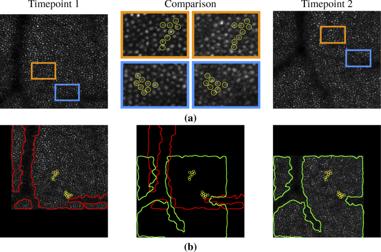
Automated longitudinal montaging of AO images remains a challenge for three primary reasons: 1) The intensity profile of cones is known to change significantly over time, even in healthy subjects [9,10] (Fig. 1(a)). This interferes with existing montaging approaches, which rely on consistent intensity information for image alignment; 2) Subtle optical and motion distortion in individual images can build up over a full montage. This prevents global alignment of full montages built at different timepoints; 3) The most prominent global feature, the pattern of blood vessel shadows on the photoreceptor mosaic, can shift between longitudinal acquisitions (Fig. 1(b)), further hindering accurate global alignment at the cellular level. Due to these limitations, manual alignments is the primary available option for longitudinal AO analysis. However, manual alignment is an expensive and time intensive task, and is generally not feasible for large scale longitudinal studies. Thus, existing studies often restrict longitudinal AO analysis to a limited number of small regions of interest across the retina [1,5] or do not require cellular alignment across time for the regions of interest [11].
Fig. 1.
Examples of image differences between AOSLO images of the same subject and retinal location between two timepoints. (a) shows individual cone intensity changes (circled in yellow) across two timepoints. (b) shows the shift of vessel shadows (outlined in red and green) relative to the corresponding cone mosaics shown in (a). The vessel outlines were found semi-automatically by Gaussian smoothing each image and then adjusting a threshold to segment the vessel regions.
To address the instability of the intensity information in longitudinally-acquired AO images, we propose using constellation features to perform alignment between such images. In contrast to intensity-based features, constellation features are constructed from the structural pattern of the cone mosaic to identify corresponding regions across time. Our proposed approach is inspired by methods originally introduced for aligning star constellations to astronomy maps [12–14], where similar challenges often arises due to atmospheric aberrations. These methods are designed to be robust to intensity variations, signal loss and spatial distortions. Using constellation features together with our previously described framework for within timepoint AO montaging [7], we are able to construct full multi-timepoint montages with accurate local cell-to-cell correspondence.
2. Methods
2.1. Method overview
Our primary focus in this work is to introduce and evaluate the use of constellation features for aligning AO images of the same subject taken at different timepoints. We first give a brief introduction to the general notations we use for image alignment and registration. In Sections 2.2–2.6 we describe how to construct constellations features and use them to align two overlapping longitudinally acquired AO images. In Sections 2.7–2.9 we describe how we adapt our previously presented within-timepoint AO montaging framework [7] to use constellation features to construct full longitudinal AO montages.
2.2. Image alignment
We begin by defining an image formally as a function that returns the intensity of the image when given a location, , within the image’s coordinate space, where . The goal of an image alignment (also known as a registration) algorithm is to align two images, and into the same coordinate space, such that corresponding objects and structures in the two images lie at the same coordinate locations. This alignment can be achieved by finding a coordinate transform, , described by the relationship,
| (1) |
which maps each location in to a corresponding location in . This transformation can be applied to the image to create the aligned image
| (2) |
by substituting the mapping described in Eq. (1) into the image function. From Eq. (2) we see that effectively serves as a “pullback” function that pulls intensity values from image into the space of image to generate a new transformed version of (denoted ) that is aligned to .
2.3. Constellation features for image alignment
Suppose that and are two nominally overlapping AO images from different timepoints. To solve for the transformation between these images, we must first be able to identify and match corresponding features across longitudinal AO images. The scale invariant feature transform (SIFT) features used in our previous work [7] are insufficient for the longitudinal case, because of the intensity variation of the cone mosaic across time (see Fig. 1). Thus, instead of matching the images by directly using intensity information, we propose using constellation features [13] constructed from the structural patterns of the cone mosaics in each image. Such features have been found to be robust to intensity differences, and have been successfully used for alignment of star constellation images to astronomical maps.
To find the constellation features for each image , we begin by finding the center locations of the cones, , in the image, where is the index for each cone in the image and is the total number of cones. In our experiments, we found cone locations using existing automated algorithms designed for cones detection in AO images. The two algorithms we evaluated are those presented by Garrioch et al. [15] and Cunefare et al. [16]. The Garrioch et al. algorithm uses spatial frequency filtering and identifies local intensity maxima in the filtered image. The Cunefare et al. algorithm uses a deep neural network trained on manually identified cone locations. Note, however, that our proposed method is agnostic as to how the cone locations are identified. It accepts the location of cone centers as a generic input. These can be obtained by means other than the two algorithms we explored, including semi-automated or manual cone location identification.
For each cone center, , we define a constellation, , as the set of all other cone center locations in the image within a radius of around . More formally,
| (3) |
Each of these constellations represents a detected cone mosaic pattern of radius within the image. We then define the constellation feature set of an image as the set of all constellations detected in the image
| (4) |
2.4. Comparing constellation features via grid matching
Given the constellation feature sets and from two images and , respectively, our goal is to compare the constellation features within these sets and find matching structural correspondences that can be used to align the two images. There are challenges associated with this task. First, due to noise, distortions and errors in cone detection, corresponding constellation features found in two different images will not match exactly. In particular, it is common that not all cones can be detected in every image, and thus many constellations can only be partially matched. In addition, each image can have thousands of features that must be compared, and the number of comparisons grows quadratically with the number of images in the dataset, which mean the individual comparisons must be implemented in a computationally efficient manner so that they can be executed rapidly.
To address these limitations, we adopt a matching technique known as grid matching, that was also originally introduced for matching star constellations [13]. In this technique, we start by fitting a sized grid with block size over each constellation, . This creates discrete block locations that span the constellation, where . For ease of computation we set as an odd multiple of to ensure that the blocks are an integer number of pixels and that there is always a center block over the center of the constellation, . Thus each block at discrete location and in the grid covers the space:
| (5) |
where and are the and elements of the center location of , respectively.
Once the grid is constructed, we check each block in the grid for the presence of a cone. If any are found, the grid location of that block is set to one, otherwise, it is set as a zero. Thus the grid block values for each constellation can be described as a function, , with values
| (6) |
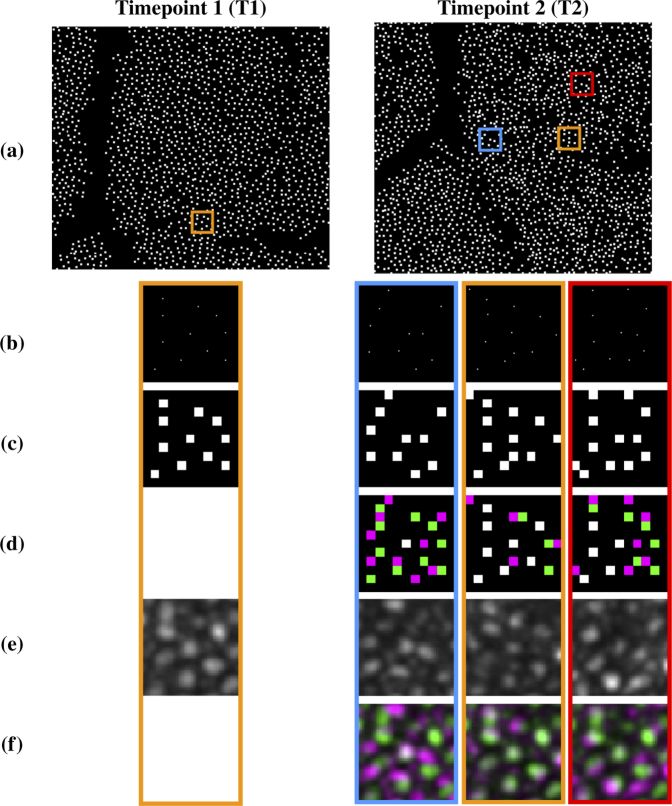
This binary grid pattern is used as a surrogate for the constellation when we are matching features between different images. Figure 2 shows several example constellations being compared using grid matching. The orange boxes show the correct matching constellations between the two images.
Fig. 2.
Visual example of how a constellation feature is constructed and compared between two images: (a) cone centers detected for the pair of longitudinal images shown in Fig. 1; (b) zoomed in regions of theboxes shown in each image in (a); (c) grid representation of the constellation feature for the center cone of each region shown in (b); (d) difference in the grid patterns for the orange region from Timepoint 1 and each region from Timepoint 2 (Green-T1 only, Magenta-T2 only, White-Both); (e) the original image intensities within each region; (f) difference in intensities within the orange region for T1 and each region for T2 (Green-T1 higher intensity, Magenta-T2 higher intensity, Gray-Similar intensities in both image). The region indicated by orange at T2 has the highest match score. Inspection of (e) and (f) indicates that it is a good match.
Grid matching has two fundamental advantages. First, the coarse representation of each constellation provides robustness when there are errors in the localization of the cone centers. For example, slight shifts in the detected cone locations across time will typically result in the same grid blocks being set to one. Second, the binary grid allows for highly efficient comparisons between the features. Given two vectorized constellation grids and , we can compare and score the fraction of matches between the features using
| (7) |
where is the logical AND operator, is the “norm” used to count the number of nonzero elements in the vector, and is the vector’s dimension, which counts the total number of elements in each vector. However, since all of the grids are identical in size, the factor in Eq. (7) is a predetermined positive constant in the algorithm that does not affect the comparisons. Thus, the score can be reduced to
| (8) |
which has an equivalent search space to Eq. (7) for finding the optimal match. can be evaluated using one AND operation and one bit summation (popcount) operation, both of which are native, single cycle instructions in modern CPUs. The efficiency of this evaluation allows us to make comparisons between all possible pairs of features in the two images to find a top match (i.e. the global maximum of the score) for each constellation. Thus for each constellation at index in image we search across all constellations at index in image for the index of the constellation that has the best match score:
| (9) |
This creates pairs of matched feature locations between the two images which we express as and associated scores . Likewise, if we search in the other direction starting from the features in images , we get the matches and scores . We then set a threshold and remove low scoring matches, so that we only retain constellation matches with high match scores. To ensure that each match is unique, we discard duplicate matches, where . Thus, we obtain a set of candidate matching locations between the two images as
| (10) |
which we will use to find the alignment transformation between the two images. Note that because the match is done in both directions, it is possible that can contain matches that partially overlap. For example, two matches can specify the same location in but different locations in . Since both of these matches cannot be accounted for by a single coordinate transform, at least one of them must be a false positive. False positives are handled by the alignment procedure described in the next section.
2.5. Alignment using random sample consensus (RANSAC)
From the previous section we are given a set of matched pairs of feature locations , where is the index across the matched pairs. Our goal is to estimate the transformation between the two image coordinate spaces using the relationship between these corresponding locations, as described in Eq. (1). If we specify to be a linear mapping, then we have
| (11) |
where
| (12) |
and
| (13) |
are the and coordinates of the pairs of matching locations from each respective image stacked in a matrix form and then transposed (denoted by the symbol in Eq. (11)). The transformation is the alignment transformation we are solving for, which has the form
| (14) |
where and are the translation in the and directions, respectively, is the rotation (in radians), and is a scaling factor. The scaling factor is included to account for potential changes in magnification between different timepoints. This value is expected to be small and is restricted in the algorithm to be be under 10% (i.e. ).
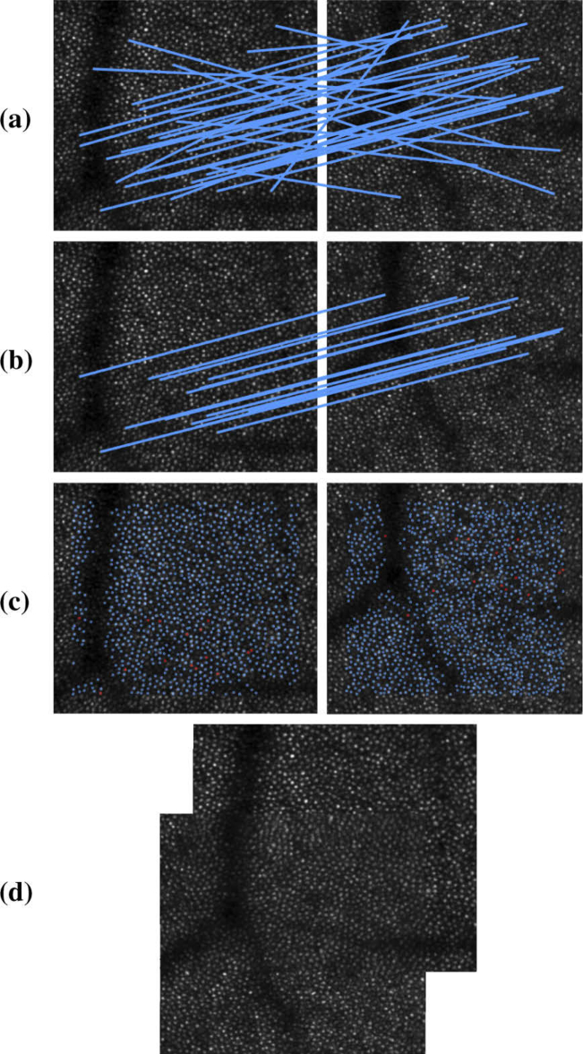
In the ideal case where the feature pairs in are perfect correspondences, Eq. (11) can be used to directly solve for the unknown alignment transformation between the images. However, we know that the matched feature pairs will contain false positive matches due to the regularity of the cone-mosiac and similarity between cone constellations. Such false positives will impact the accuracy of the transformation estimation and must be removed for accurate cell-to-cell alignment. To address this problem, we use a technique known as random sample consensus (RANSAC) [17] to remove outlier matches, which has been effective for within timepoint AO montaging [6–8]. The goal of RANSAC is to estimate multiple prospective transformations, , from random subsets of matched feature pairs in . These transformations are then tested against the full set of matches and the that aligns the highest number of candidate matched feature pairs within tolerance is considered the final transformation (). Figure 3 shows an example alignment between two images obtained using constellation features. Figure 3(a) shows all of the candidate matches. Figure 3(b) shows the inlier matches associated with the best transformation estimated by RANSAC. Figure 3(c) shows the location of every detected constellation feature. The locations of the inlier matched feature pairs used by RANSAC to estimate the final transformation are highlighted in red. The mean intensity of the two images after performing the alignment is shown in Fig. 3(d).
Fig. 3.
Example of an alignment between two longitudinal images using the constellation feature. (a) shows the total matches found. (b) shows the inlier matches found after RANSAC. (c) shows the location of features found in each image, with those in red showing the features in the two images corresponding to the inlier matches. (d) shows the average of the two images after alignment.
2.6. Rotation in constellation features
One additional consideration we need to take into account when using constellation features is that eye position changes can cause the same underlying constellation to have a different rotational orientation across images. To account for this in practice, we enhance the feature set for each image by including reoriented versions of each constellation feature . To ensure that these reoriented constellations are rotated in a consistent manner, we first find the vector
| (15) |
between the constellation center and its closest neighboring cone location . We use this vector to rotate the constellation such that the cone closest to the center will always lie on the x-axis. We accomplish this by solving for a rotational transformation
| (16) |
that will align to the unit vector in the x direction, , where
| (17) |
is the angle between the two vectors, and is the four-quadrant inverse tangent function. Centering this rotation on , we can then generate the reoriented constellation
| (18) |
Due to possible errors in the cone detection, the closest neighbor may not always be detected in the image. To help mitigate such errors, we repeat this reorientation for , which are the indices for the closest cone centers to in constellation . We then include each reoriented constellation as an additional feature for the image. This updates the total feature set defined in Eq. (4) to be
| (19) |
which is the set of all constellations and their duplicates in different orientations.
2.7. Longitudinal montaging framework
To create a full longitudinal AO montage, we use the constellation-based alignment method proposed in the previous sections to expand on the framework we previously developed for within timepoint AO montaging [7]. While this section will summarize and reintroduce the key concepts of the framework relevant to our approach, we refer the reader to the original paper for more details.
For a given longitudinal AOSLO dataset, we describe each image in the dataset as , where is the nominal retinal location of the image (determined by the fixation location during acquisition), is the index for the timepoint the image was acquired at, and is the AO modality of the image (confocal [18], split detection [19], and dark-field [20]). Expanding on the notation from the previous section, each image returns the intensity of the image given the pixel location, , within each image’s coordinate space. We note that each coordinate space, , is specific to the location, , and time, , an image was acquired at, but is independent of the modality of the image. This is because all three AO modalities are acquired simultaneously and share the same coordinate space for a given location and time.
The goal of our algorithm is to align every image in the dataset into a single global coordinate space, common across fixation locations and time. We refer to this as the reference space, , which we select (without loss of generality) as the pixel coordinate space of image, , in the dataset located closest to the origin of the fixation coordinate grid () taken at the first timepoint (). Analogous to Eq.(1), we represent the alignment of each image through a transformation mapping,
| (20) |
where maps each location in to a corresponding location in . And analogous to Eq. (2), this transformation can be applied to the image to create the aligned image
| (21) |
by substituting the relationship between the coordinate systems described in Eq. (20) into the image function.
2.8. Composing relative transformations
For images that directly overlap with , we use the constellation alignment method we presented in the previous sections to solve for . However, for images in the dataset that do not overlap with there is no information to find the transformation directly. Thus, these transformations must be found indirectly by first solving for the relative local transformations between adjacent images that do overlap, and then chaining together these relative transformations to create a global transformation for each image into the reference space. For images that are from the same timepoint as the reference image (i.e. ), we can describe this global transformation for an image at location as
| (22) |
which represents a composition of the relative transformations between nominally adjacent images starting from location and ending at the origin. Since these images are all from the same timepoint, we can use our previously presented montaging algorithm [7] to solve for these relative transformations.
However, for images that are from a different timepoint than the reference image (i.e. ) we must consider which spatiotemporal path we take to connect the image to the reference frame. For example, one possibility is to first align the image to other images within the same timepoint until it is connected to the origin and then align across timepoints at the origin. Alternatively, we can first align the image across timepoints at its nominal location and then use the transformations from Eq. (3) to reach the reference frame. It is worth noting that in the ideal case, where there are no errors in the transformations, any choice of spatiotemporal path that connected two images should result in the same global transformation. However, in practice, accumulation of errors during the composition can lead to different results between these different path choices.
In our algorithm we chose the path where alignment across time is first performed individually at each nominal location. This can be described by extending Eq. (3) to include an additional transformation between timepoints in the composition,
| (23) |
Our reasoning for this decision is motivated by a primary goal of longitudinal analysis, which is to observe cellular level change. For this case we want to minimize the amount of alignment error between images of the same retinal location, when making observations across time. Thus, we chose a spatiotemporal path where there is only a single transformation between images at the same nominal location from different timepoints. This also has the advantage of allowing us to specify a region of interest (ROI) on the baseline montage () and having all measurements at the same location from later timepoints be directly aligned to that ROI.
2.9. Matching criterion and discontinuity detection
Two considerations the algorithm needs to take into account when constructing the full AO montage is how to decide which image (and thus transformation) to use when multiple images are overlapping, and how to determine when there was a discontinuity in retinal coverage during data acquisition and, in such cases, to reject all of the potential transformations. In our previous work [7] we determined a set of criteria based on the number of inlier matches and the number of total matches to set the threshold for a valid match. The primary difference here is that we have found that constellation features tend to generate both more overall matches and more false positive matches, both of which reduced the relative inlier match percent for valid alignments. To accommodate for this change we have relaxed the threshold for minimum percentage of inlier matches from 10% for the within timepoint case to 5% when aligning with constellation features.
3. Experiments
3.1. Data and default algorithm parameters
The equipment and image acquisition protocol used in this study have been described in detail previously [5,18,19,21]. To summarize, a scanning laser ophthalmoscope equipped with AO was used to acquire high-resolution images of the retina. Images were acquired at 16.7 Hz using 795 nm imaging light, with images in three modalities (confocal, split detection, and dark field) acquired simultaneously. Image sequences were 150 frames in length and were 1° by 1° of visual angle in spatial extent.
The research protocol for our experimental data was approved by the institutional review board at the University of Pennsylvania and the Children’s Hospital of Philadelphia, and the study adhered to the tenets of the Declaration of Helsinki. All light exposures were below the maximum permissible limits specified by the American National Standards Institute [22]. All subjects provided informed consent. Subjects’ pupils were dilated (phenylephrine hydrochloride, 2.5%, and tropicamide, 1%) prior to image acquisition. Axial lengths for all eyes were measured at each timepoint using an IOL Master (Carl Zeiss Meditec, Dublin, CA) and were used to calculate the scale of the AOSLO images at each timepoint.
Eight eyes from eight normal sighted volunteers were imaged at two timepoints (6-12 months apart). Images were collected across the horizontal and vertical meridians of the retina from the fovea out to approximately 1800m eccentricity, with additional images collected in the central 600m by using the corners of the scanning square as the fixation location. Four of the longitudinal datasets were used for the development of the algorithm. The remaining four datasets were held in reserve to test the algorithm after an optimal set of parameters was determined.
Unless otherwise stated, in each experiment we used the following default algorithm parameters: 70 pixel constellation window size (W = 70), 5 pixels constellation grid size (G = 5), 6 pixel RANSAC tolerance ( = 6), 10 degree limitation on rotation () , 10% limitation on scaling (0.9 < L < 1.1), 3 constellation reorientation variations (R = 3), and a 20% constellation feature matching threshold ().
3.2. Preprocessing and distortion correction
Image sequences at each location were combined into a single image by aligning and averaging a minimum of 50 frames from the image sequence relative to a reference frame. Each reference frame was automatically selected using a custom algorithm based on the method described by Solomon et al. [23]. Image sequences were desinusoided using an image of a Ronchi ruling of equally spacing lines, and strip registered to the reference frame to correct for intra-frame distortions from eye motion during scanning image acquisition [24]. We corrected for distortions present in the reference frame, using a custom algorithm based on the method described by Bedggood and Metha [25], where the median eye motion throughout a given image sequence is assumed to be zero. More specifically, we estimated the distortions contained within the reference frame by finding the median translation required to register 49 frames of the image sequence to each strip of the reference frame, and then fixing the distortion in the reference frame in the equal yet opposite direction.
3.3. Longitudinal montaging
We ran our proposed montaging algorithm on each of the four longitudinal development datasets to construct four pairs of full longitudinal montages. As described in Sec. 2.8, the baseline montage was constructed using our SIFT-based approach [7], and the proposed constellation features were used to align each image from the second timepoint to an image in the baseline montage.
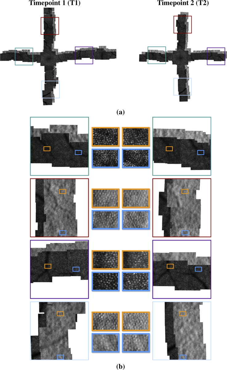
A trained, experienced rater (MC) qualitatively assessed each montage at 5 locations– one location on each of the four arms and one location at the fovea. For each location in the arms for all four montages, the rater found that the algorithm produced clear cell-to-cell alignments between the first and second time point. The foveal locations showed varying degrees of success. Cell-to-cell alignment could be established in portions of the image, but the tightly packed cell pattern and reduced visibility of cones near the foveal center degraded the overall quality of the alignment. Figure 4(a) shows the montages for the baseline (T1) and second (T2) timepoint from one of the longitudinal datasets. Figure 4(b) shows zoomed in regions of this montage, demonstrating the cell-to-cell correspondence between the montages.
Fig. 4.
Example of a longitudinal montage between two AO datasets collected a year apart: (a) montages of the confocal images from each timepoint; (b) zoomed in regions showing the cell-to-cell correspondence after alignment. The first and third rows show the confocal modality of the montage, and the second and fourth rows show the split detection modality.
To assess the montages quantitatively, for each dataset we evaluated the image similarity between each image in the second timepoint and the baseline image, across the overlapping regions between the images. The metric we used for this evaluation was the normalized mutual information (NMI) [26] between the images. NMI is a statistical measure of the agreement between the images that is robust with respect to overall intensity variation [27]. This makes it a reasonable choice for evaluating longitudinal AO image alignment where the cone intensities are known to vary over time. Note, however, that NMI only offers a global evaluation of the statistical similarities between the images intensities. Thus it is an imperfect metric for determining local cell-to-cell alignment. This is a limitation of all image similarity metrics of which we are aware. If we had a metric of image similarity that was robust to the type of variation in individual cone intensities that occur across AO images, we could use it directly as a cost function in the longitudinal montaging algorithm.
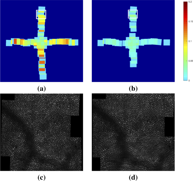
Figure 5(a) shows a map of the NMI at each of the overlapping regions in the longitudinal montage created using the proposed method. For comparison, Fig. 5(b) shows the same map when SIFT was used to perform the longitudinal alignment. In the SIFT case, we see that many of the areas are missing because the alignment could not meet the minimum threshold criterion for the number and percentage of inlier matches found between the images. For the cases that did produce sufficient matches for alignment, we see that the image similarity in the overlapping region after alignment is much lower than when using the constellation feature algorithm. In Fig. 5(c) and (d), we show the average confocal intensity between the overlapping images located at the white box in (a) and (b), respectively. We see that the average is considerably more blurred in the SIFT montage due to the image misalignment.
Fig. 5.
Maps of the NMI in the overlapping regions of the second timepoint montage after longitudinal alignment to the first timepoint using (a) our proposed constellation method and (b) a SIFT-based approach. Missing areas in the map in (b) indicate areas where the images could not be aligned due to not finding enough inlier matches to meet the alignment criterion. (c) and (d) show the average confocal intensity of the overlapping images located at the white boxes in (a) and (b), respectively.
3.4. Alignment accuracy and robustness
To quantitatively evaluate the accuracy and robustness of the proposed algorithm, we manually selected 20 longitudinal image pairs (5 image pairs from each development dataset), where each pair was known to spatially overlap. The 5 locations for each dataset were selected to be at different eccentricities, with roughly equal spacing from the fovea to the furthest extent of the dataset (1800 m). One of the four arms in the dataset was randomly selected for each eccentricity. Using this development dataset, we evaluated the performance of the image alignments when using different constellation sizes, approaches to cone detection, AO modalities, and degrees of cone loss. For each case we evaluated the NMI between the images after alignment as a metric of alignment accuracy.
3.4.1. Optimal constellation and grid size
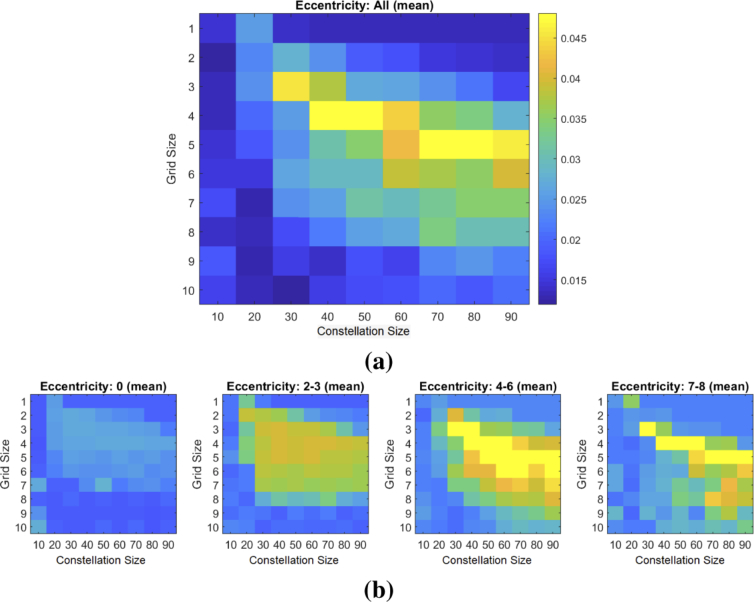
We evaluated the effect that the size of the constellation and grids has on the accuracy of the final alignment. For each of the 20 image pairs, we performed the image alignment using constellation features of sizes (W) ranging from 10 to 90 pixels (in increments of 10) and grid sizes (G) ranging from 1 to 10 pixels (in increments of 1). Figure 6(a) shows a plot of the mean relationship between alignment accuracy, constellation size and grid size. The intensity of each square in the plot shows the mean NMI over the 20 pairs for a given constellation size and grid size. Figure 6(b) shows the mean relationship when we bin the results according to the nominal eccentricity (in degrees) at which the images were acquired.
Fig. 6.
Matrices showing (a) the mean image similarity (NMI) after the alignment when using different constellation sizes (x-axis) and grid size (y-axis) for aligning the 20 development image pairs. (b) shows the mean image similarity when the image pairs are binned according to the eccentricity (in degrees) at which they were acquired.
From these results we see that the optimal operating range for the algorithm on our images is with a constellation size of 60-70 pixels and a grid size of 4-6 pixels. This optimal range does not appear to be strongly dependent on eccentricity. However, we observe that the global performance of the algorithm is sensitive to the eccentricity of the images. In Section 4, we will discuss the potential reasons for this dependence.
3.4.2. Choice of cone detection algorithm and image modalities
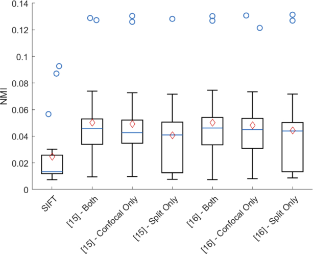
Next, we evaluated the effect that the cone detection algorithm and the modalities used in the alignment have on the algorithm accuracy. For each of the 20 image pairs in the development dataset, we evaluated the alignment using the cone detection methods by Garrioch et al. [15] and Cunefare et al. [16] with just the confocal images, just the split images, and both confocal and split images as the input. Figure 7 shows a comparison of the NMI for each of these cases across the 20 pairs. We see that the algorithm performance is roughly equivalent for both cone detection methods, and using both the split and confocal images together had the best average performance. Also shown in the plot is a comparison against the intensity-based montaging algorithm using SIFT features [7].
Fig. 7.
Comparison of the NMI image similarity (across 20 image pairs) after longitudinal alignment by SIFT [7] and the proposed constellation algorithm when using different automated cone detection inputs (Garrioch et al. [15] or Cunefare et al. [16]), and different AO imaging modalities as inputs (confocal only, split detection only, or both). The box plot show the median, 25th and 75th percentiles, and non-outlier range (whiskers) of the data. Blue circles show the outlier points, and the red diamond show the mean of the data.
3.4.3. Effect of cone loss
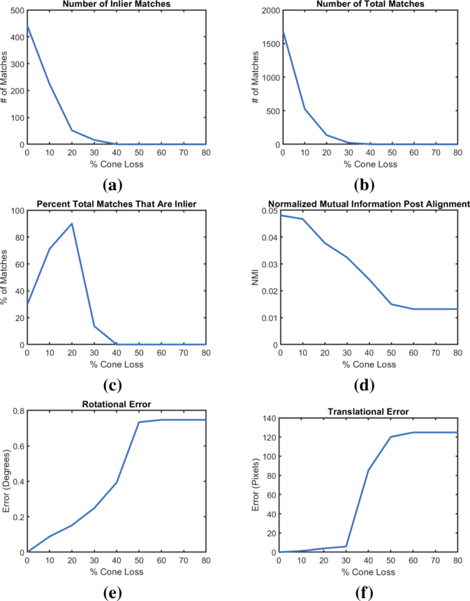
Due to potential noise, artifacts, image quality, and subject motion it is not always possible for a cone detection method to correctly locate every cone center in an image. Thus, we evaluated the effect that cone loss has on the performance of the alignment. Using the 20 selected image pairs from the development dataset, we evaluated the automated alignment by our proposed algorithm with different percentages (0% 20% 40% 60% 80%) of the detected cone centers randomly removed from both images before construction of the constellation features. For this experiment, we used the cones detected through Cunefare et al.’s [16] approach as the baseline. Figure 8 shows six algorithm metrics as a function of the percent cone loss including: total number of inlier and outlier matches found and their ratio, the image similarity after alignment, and the relative rotational and translational error compared to the cases where the algorithm was run without simulated cone loss. We see from these plots that, in general, the algorithm can perform alignments with low translational and rotational error up to a 30% cone loss, at which point the performance starts decreasing rapidly. In addition, we that see that the point at which the algorithm starts to perform worse is generally consistent across all six metrics. We note also that our method appears to be reasonably robust to the total number of matches and inlier matches available for alignment. In Fig. 8, at 30% cone loss, we see that the median number of total matches dropped from 1700 to less than 50, and the median number of inlier matches dropped from 430 to less than 20. Yet, at this same level of cone loss, the translation error remained under 8 pixels, and the rotational error remained under 0.2 degrees.
Fig. 8.
Analysis of the robustness of the constellation features. Each plot shows the median (across the 20 test pairs) of the relationship between the percent cone loss in the input image and the total number of (a) inlier (larger is better) and (b) total (larger is better) matches found, (c) percent of total matches that are inlier (larger is better), (d) NMI between the images after alignment (larger is better), and the (e) rotational and (f) translational errors (smaller is better) relative to when there are no simulated cone loss.
3.4.4. Evaluation of withheld dataset against manual alignments
In our final experiment, we evaluated our algorithm using the 4 test datasets (20 image pairs) that were withheld during the development of the algorithm. For each dataset, the 5 longitudinal image pair locations were chosen as follows: one located at each of 150m, 300m, and 600m temporal to fixation; one located as far temporal to the fovea as possible (at 1350 m, 900 m, 1960 m, and 1640 m); and one variable location for each subject (900 m, 450 m, 1200 m and 1200 m temporal to fixation, respectively). The goal of this experiment was to assess if the algorithm parameters chosen during development could be generalized to new datasets. In addition, we report a comparison between the automated alignments and manual alignments constructed by a trained rater.
For this experiment both confocal and split detection modalities were used in the alignment. The constellation features were constructed using cones detected automatically via Cunefare et al. [16]. The results of the experiment were evaluated against manually constructed alignments of the 20 pairs through the following metrics: NMI between the overlapping regions after alignment, and the difference of the rotation, translation and scale of the transformations found for the manual and automated alignments. This evaluation was performed double-blind, where neither the algorithm operator (MC) nor the manual rater (JIWM) were allowed to observe each others’ alignments before the final comparison between the automated and manual alignments. This experiment was preregistered at https://osf.io/hmt5j/, prior to manual or automated evaluation of the images.
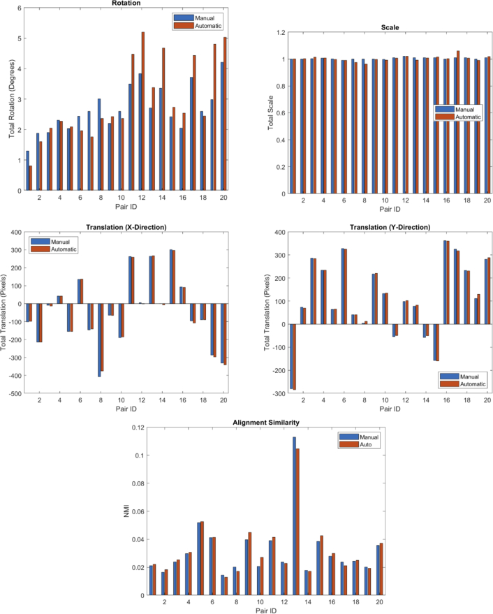
Upon completion of the preregistered automated alignments (but before evaluating against the manual alignments) we observed that the algorithm was failing on many of the new images located in the periphery of the retina. Post-hoc analysis showed that the primary reason for this was that the confocal images in the new datasets provided better visualization of the rod cells. This resulted in rods being falsely identified as cones by the automated cone identification software. As a consequence, the longitudinal alignment algorithm had additional false positives in the constellation feature matches that prevented RANSAC from finding the correct transformation. To address this, we made a post-hoc adjustment to the RANSAC sampling parameter that enforced equal sampling from each image modality. This generated candidate transformations from the matches in both modalities, thus preventing the false positives in the confocal images from completely overriding the correct matches found in the split detection (where the rods were not as apparent). We verified that this algorithm modification did not appreciably change the results obtained with the original development dataset. We then compared the manual alignments to the automated alignments after this adjustment (Fig. 9). The results showed excellent agreement, both in terms of NMI and in terms of the alignment transformation parameters. The largest differences, apparent in the figure, are in the rotational parameter, where the two methods can differ by as much as 2 degrees. The manual rater noted that it is very difficult to simultaneously determine rotation and scale parameters that cause two image regions to match across the entire overlapping region, and we regard the differences between the two methods as within a reasonable margin of error.
Fig. 9.
Comparison between the manual and automated alignment for the 20 withheld test dataset image pairs. Shown are the plots for the rotation, scale and translation values for the alignment transformation, and the intensity similarity (using NMI) of the overlapping regions after each alignment.
4. Discussion
4.1. Algorithm performance
Our evaluation results suggest that our proposed algorithm can produce highly accurate automated montages of AO longitudinal images. This is demonstrated qualitatively in Fig. 4, where we can see that the montage was aligned cell-to-cell across multiple arms of the montage. This is an improvement over current practice, where typically the montages are created independently at each timepoint and then globally aligned, and manually adjusted for each region of interest. In such cases, the alignment error will often accumulate across the montage and prevent cell-to-cell alignment at one end of montage depending on where the global alignment is optimized.
Our quantitative analysis of the alignment accuracy, shown in Fig. 9, further supports the good performance of our algorithm. We see from the comparison of the transformation parameters and alignment similarity that the automated alignments agree well with the manual alignments for each of the image pairs. We observe that the primary differences between the manual and automated alignments is expressed in the rotational component of the transformation. However, we note that while the relative difference appears large in the figure, the absolute error does not exceed 2 degrees. These small alignment parameter differences between the automated and manual alignments do not appear to result in substantial differences in alignment NMI. In fact, of the 20 image pairs, the algorithm was able to find an alignment with a better image similarity than the manual rater in 12 of the 20 cases. This highlights the challenge of finding the correct alignment between longitudinal AO images. Even for a well trained and experienced manual rater, the inherent longitudinal intensity variation and residual distortions in the images can result in uncertainties regarding the correct alignment.
4.2. Limitations
The primary limitation of our proposed algorithm is in its reliance on accurate cone locations for the constellation feature construction. Failures in cone detection, both false positives and false negatives, can translate to a decrease in alignment performance. From Fig. 8 we see that in general the algorithm is fairly robust when there is less than 30 percent cone detection failure. However, beyond 30 percent loss we see a rapid drop in performance. This may make alignment problematic for images from subjects with retinal pathology and cone degeneration, where cone detection is more challenging and the number of detected cones is expected to change over time because of the disease. For such cases, it may be possible to extend the montaging framework to use areas with intact cone moasics to help align areas where cone loss impairs alignment.
In Fig. 6 we see that the global performance of the algorithm can depend on the nominal eccentricity at which the images were acquired. For large eccentricities, the decrease in performance comes mostly from errors in automated cone detection. The more prominent (yet inconsistent) visibility of rods at large eccentricities often leads to false positive detections, which directly interferes with the constellation feature construction. In addition, the deep learning based cone detection algorithm [16] was not originally trained to detect cones at locations outside of the parafovea. Retraining of the algorithm using examples from these locations can potentially help address the performance loss. This could be helpful for cone identifications in general, since even manual raters show lower agreement in making cone identifications at higher eccentricities due to rod infiltration. [21]
Conversely, near the fovea, cones are usually detected accurately, but the alignment suffers due to a lack of unique constellation patterns. At these locations, the cones are tightly packed into a regular pattern, which causes many of the constellation features to be similar to each other. This may lead to too many false positive matches for RANSAC to identify the correct inlier transformation.
The impact of these limitations was observed in our final experiment using a withheld dataset. We saw that the RANSAC sampling parameter had to be adjusted for the new dataset in order for the algorithm to operate correctly. It is important to keep the possibility of such adjustments, which can be easily implemented, in mind when applying the algorithm to future datasets or patient cases.
Lastly, it is worth noting that any similarity metric we use in our analysis is also inherently affected by the number of cones in the image (and therefore, the eccentricity at which it was acquired). This is due to the fact that the cone reflectivity changes across timepoints, but the intercellular space remains dark. Thus, even when perfectly aligned, longitudinal foveal images will have less similarity with each other than longitudinal images at higher eccentricities will have with each other. As noted before, this is an additional reason why using intensity-based image similarity measures directly for longitudinal AO montaging is problematic.
5. Conclusion
We have presented a fully automated framework for longitudinal montaging of AO images across timepoints. For alignment, our method uses features constructed from constellations of cone patterns, which are more robust to cone reflection changes than intensity-based alignment algorithms. Our results show that the algorithm produces accurate pairwise alignment and is able to construct full cell-to-cell longitudinal AO montages. The constellation features and montaging algorithm proposed in this paper is available as open-source software and can be downloaded at: https://github.com/BrainardLab/AOAutomontaging.
Acknowledgments
We thank Dr. Alfredo Dubra for sharing the adaptive optics scanning laser ophthalmoscopy optical design as well as adaptive optics control, image acquisition, and image registration software, and Ms. Grace Vergilio and Ms. Yu You Jiang for their assistance with the data collection and image analysis.
Funding
National Eye Institute10.13039/100000053 (P30 EY001583, R01 EY028601, U01 EY025477); Foundation Fighting Blindness10.13039/100001116 (Research To Prevent Blindness Award); F. M. Kirby Foundation10.13039/100001205; Paul MacKall and Evanina Bell MacKall Trust10.13039/100008556.
Disclosures
RFC is an inventor on a provisional patent and is a consultant for Translational Imaging Innovations (P,C). DHB is an inventor on a provisional patent (P). JIWM is an inventor on US Patent 8226236 and a provisional patent and receives funding from AGTC (F,P).
References
- 1.Talcott K. E., Ratnam K., Sundquist S. M., Lucero A. S., Lujan B. J., Tao W., Porco T. C., Roorda A., Duncan J. L., “Longitudinal study of cone photoreceptors during retinal degeneration and in response to ciliary neurotrophic factor treatment,” Invest. Ophthalmol. Vis. Sci. 52(5), 2219–2226 (2011). 10.1167/iovs.10-6479 [DOI] [PMC free article] [PubMed] [Google Scholar]
- 2.Hansen S., Batson S., Weinlander K. M., Cooper R. F., Scoles D. H., Karth P. A., Weinberg D. V., Dubra A., Kim J. E., Carroll J., Wirostko W. J., “Assessing photoreceptor structure following macular hole closure,” Retin. Cases Brief Rep. 9(1), 15–20 (2015). 10.1097/ICB.0000000000000117 [DOI] [PMC free article] [PubMed] [Google Scholar]
- 3.Chui T. Y. P., Pinhas A., Gan A., Razeen M., Shah N., Cheang E., Liu C. L., Dubra A., Rosen R. B., “Longitudinal imaging of microvascular remodelling in proliferative diabetic retinopathy using adaptive optics scanning light ophthalmoscopy,” Ophthal Physl. Opt. 36(3), 290–302 (2016). 10.1111/opo.12273 [DOI] [PMC free article] [PubMed] [Google Scholar]
- 4.Langlo C. S., Erker L. R., Parker M., Patterson E. J., Higgins B. P., Summerfelt P., Razeen M. M., Collison F. T., Fishman G. A., Kay C. N., Zhang J., Weleber R. G., Yang P., Pennesi M. E., Lam B. L., Chulay J. D., Dubra A., Hauswirth W. W., Wilson D. J., Carroll J., “Repeatability and longitudinal assessment of foveal cone structure in cngb3-associated achromatopsia,” Retina 37(10), 1956–1966 (2017). 10.1097/IAE.0000000000001434 [DOI] [PMC free article] [PubMed] [Google Scholar]
- 5.Jackson K., Vergilio G. K., Cooper R. F., Ying G.-S., Morgan J. I., “A 2-year longitudinal study of normal cone photoreceptor density,” Invest. Ophthalmol. Vis. Sci. 60(5), 1420–1430 (2019). 10.1167/iovs.18-25904 [DOI] [PMC free article] [PubMed] [Google Scholar]
- 6.Li H., Lu J., Shi G., Zhang Y., “Automatic montage of retinal images in adaptive optics confocal scanning laser ophthalmoscope,” Opt. Eng. 51(5), 057008 (2012). 10.1117/1.OE.51.5.057008 [DOI] [Google Scholar]
- 7.Chen M., Cooper R. F., Han G. K., Gee J., Brainard D. H., Morgan J. I., “Multi-modal automatic montaging of adaptive optics retinal images,” Biomed. Opt. Express 7(12), 4899 (2016). 10.1364/BOE.7.004899 [DOI] [PMC free article] [PubMed] [Google Scholar]
- 8.Davidson B., Kalitzeos A., Carroll J., Dubra A., Ourselin S., Michaelides M., Bergeles C., “Fast adaptive optics scanning light ophthalmoscope retinal montaging,” Biomed. Opt. Express 9(9), 4317–4328 (2018). 10.1364/BOE.9.004317 [DOI] [PMC free article] [PubMed] [Google Scholar]
- 9.Pallikaris A., Williams D. R., Hofer H., “The reflectance of single cones in the living human eye,” Invest. Ophthalmol. Vis. Sci. 44(10), 4580–4592 (2003). 10.1167/iovs.03-0094 [DOI] [PubMed] [Google Scholar]
- 10.Mariotti L., Devaney N., Lombardo G., Lombardo M., “Understanding the changes of cone reflectance in adaptive optics flood illumination retinal images over three years,” Biomed. Opt. Express 7(7), 2807–2822 (2016). 10.1364/BOE.7.002807 [DOI] [PMC free article] [PubMed] [Google Scholar]
- 11.Foote K. G., Loumou P., Griffin S., Qin J., Ratnam K., Porco T. C., Roorda A., Duncan J. L., “Relationship between foveal cone structure and visual acuity measured with adaptive optics scanning laser ophthalmoscopy in retinal degeneration,” Invest. Ophthalmol. Vis. Sci. 59(8), 3385–3393 (2018). 10.1167/iovs.17-23708 [DOI] [PMC free article] [PubMed] [Google Scholar]
- 12.Duan Y., Niu Z., Chen Z., “A star identification algorithm for large fov observations,” in “Image and Signal Processing for Remote Sensing XXII,” vol. 10004 (International Society for Optics and Photonics, 2016), p. 100041G. [Google Scholar]
- 13.Padgett C., Kreutz-Delgado K., “A grid algorithm for autonomous star identification,” IEEE Trans. Aerosp. Electron. Syst. 33(1), 202–213 (1997). 10.1109/7.570743 [DOI] [Google Scholar]
- 14.Hernández E. A., Alonso M. A., Chávez E., Covarrubias D. H., Conte R., “Robust polygon recognition method with similarity invariants applied to star identification,” Adv. Space Res. 59(4), 1095–1111 (2017). 10.1016/j.asr.2016.11.016 [DOI] [Google Scholar]
- 15.Garrioch R., Langlo C., Dubis A. M., Cooper R. F., Dubra A., Carroll J., “The repeatability of in vivo parafoveal cone density and spacing measurements,” Optom. Vis. Sci. 89(5), 632–643 (2012). 10.1097/OPX.0b013e3182540562 [DOI] [PMC free article] [PubMed] [Google Scholar]
- 16.Cunefare D., Fang L., Cooper R. F., Dubra A., Carroll J., Farsiu S., “Open source software for automatic detection of cone photoreceptors in adaptive optics ophthalmoscopy using convolutional neural networks,” Sci. Rep. 7(1), 6620 (2017). 10.1038/s41598-017-07103-0 [DOI] [PMC free article] [PubMed] [Google Scholar]
- 17.Fischler M. A., Bolles R. C., “Random sample consensus: a paradigm for model fitting with applications to image analysis and automated cartography,” Commun. ACM 24(6), 381–395 (1981). 10.1145/358669.358692 [DOI] [Google Scholar]
- 18.Dubra A., Sulai Y., “Reflective afocal broadband adaptive optics scanning ophthalmoscope,” Biomed. Opt. Express 2(6), 1757–1768 (2011). 10.1364/BOE.2.001757 [DOI] [PMC free article] [PubMed] [Google Scholar]
- 19.Scoles D., Sulai Y. N., Langlo C. S., Fishman G. A., Curcio C. A., Carroll J., Dubra A., “In vivo imaging of human cone photoreceptor inner segments,” Invest. Ophthalmol. Vis. Sci. 55(7), 4244–4251 (2014). 10.1167/iovs.14-14542 [DOI] [PMC free article] [PubMed] [Google Scholar]
- 20.Scoles D., Sulai Y. N., Dubra A., “In vivo dark-field imaging of the retinal pigment epithelium cell mosaic,” Biomed. Opt. Express 4(9), 1710–1723 (2013). 10.1364/BOE.4.001710 [DOI] [PMC free article] [PubMed] [Google Scholar]
- 21.Morgan J. I., Vergilio G. K., Hsu J., Dubra A., Cooper R. F., “The reliability of cone density measurements in the presence of rods,” Trans. Vis. Sci. Tech. 7(3), 21 (2018). 10.1167/tvst.7.3.21 [DOI] [PMC free article] [PubMed] [Google Scholar]
- 22.Standard A., “American national standard for the safe use of lasers. American National Standards Institute, Inc.,” New York (1993).
- 23.Salmon A. E., Cooper R. F., Langlo C. S., Baghaie A., Dubra A., Carroll J., “An automated reference frame selection (arfs) algorithm for cone imaging with adaptive optics scanning light ophthalmoscopy,” Trans. Vis. Sci. Tech. 6(2), 9 (2017). 10.1167/tvst.6.2.9 [DOI] [PMC free article] [PubMed] [Google Scholar]
- 24.Dubra A., Harvey Z., “Registration of 2D images from fast scanning ophthalmic instruments,” in “Proc. of 2010 International Workshop on Biomedical Image Registration,” (Springer, 2010), pp. 60–71 [Google Scholar]
- 25.Bedggood P., Metha A., “De-warping of images and improved eye tracking for the scanning laser ophthalmoscope,” PLoS One 12(4), e0174617 (2017). 10.1371/journal.pone.0174617 [DOI] [PMC free article] [PubMed] [Google Scholar]
- 26.Studholme C., Hill D. L., Hawkes D. J., “An overlap invariant entropy measure of 3D medical image alignment,” Pattern Recogn. 32(1), 71–86 (1999). 10.1016/S0031-3203(98)00091-0 [DOI] [Google Scholar]
- 27.Pluim J. P., Maintz J. A., Viergever M. A., “Mutual-information-based registration of medical images: a survey,” IEEE Trans. Med. Imag. 22(8), 986–1004 (2003). 10.1109/TMI.2003.815867 [DOI] [PubMed] [Google Scholar]


