DIAGNOSIS STATUS GUIDED BRAIN IMAGING GENETICS VIA INTEGRATED REGRESSION AND SPARSE CANONICAL CORRELATION ANALYSIS

Abstract

Brain imaging genetics use the imaging quantitative traits (QTs) as intermediate endophenotypes to identify the genetic basis of the brain structure, function and abnormality. The regression and canonical correlation analysis (CCA) coupled with sparsity regularization are widely used in imaging genetics. The regression only selects relevant features for predictors. SCCA overcomes this but is unsupervised and thus could not make use of the diagnosis information. We propose a novel method integrating regression and SCCA together to construct a supervised sparse bi-multivariate learning model. The regression part plays a role of providing guidance for imaging QTs selection, and the SCCA part is focused on selecting relevant genetic markers and imaging QTs. We propose an efficient algorithm based on the alternative search method. Our method obtains better feature selection results than both regression and SCCA on both synthetic and real neuroimaging data. This demonstrates that our method is a promising bi-multivariate tool for brain imaging genetics.

1. Introduction

Brain imaging genetics has grown rapidly during the past decade. It combines both genetics factors, e.g., the single nucleotide polymorphisms (SNPs), and imaging quantitative traits (QTs). Using imaging QTs as endophenotypes could improve the identification ability, and offer new opportunities to interpret the causality of relationships between genetic variations and brain structure, function and abnormality such as Alzheimer’s disease (AD) [1, 2].

In biomedical studies, the sparse regression techniques usually take genetic markers or imaging QTs as predictors, and the diagnosis status as responses for identifying diagnosis-relevant biomarkers. They only select variables for predictors. Sparse canonical correlation analysis (SCCA) is one of the most popular bi-multivariate method in imaging genetics. The SCCA methods identify bi-multivariate associations between two or among more-than-two sets of variables [3, 4, 5, 6]. Unfortunately, SCCA is unsupervised method indicating that it cannot make use of the diagnosis status information. To construct the supervised SCCA, the three-way SCCA has been proposed. It maximizes pairwise correlations among SNPs, QTs and the diagnosis status. From the point of view of optimization, modeling this complexity relationship among three sets of variables could reduce the performance, since it requires those extracted SNPs are correlated to both imaging QTs and diagnosis information simultaneously.

In this study, we propose a novel method which combines SCCA and regression (sCCAR). In our method, the regression part plays a role of providing guidance for imaging QTs selection, while the SCCA part is focused on selecting relevant SNPs and imaging QTs. This modeling method is quite useful since it transforms the conventional SCCA to be guided by the diagnosis status. The alternating search method is employed to solve the sCCAR as it is bi-convex. Using both synthetic and real neuroimaging data, sCCAR obtains better or equal correlation coefficients, but holds better canonical weight profiles. This indicates that sCCAR outperforms both regression and SCCA, demonstrating it could be a promising bi-multivariate tool for brain imaging genetics.

2. METHOD

We denote scalars as italic letters, column vectors as boldface lowercase letters, and matrices as boldface capitals.

2.1. IDENTIFYING RELEVANT QTs VIA SPARSE REGRESSION

In brain imaging genetics, let $Y\in {\mathcal{R}}^{n\times q}$ be the matrix of imaging QTs with n subjects and q QTs, and z be the diagnosis status, the regression model

$$\underset{v}{\min }\frac{1}{2}\Vert z-Yv{\Vert }_2^2+{\lambda }_v\Omega (v)$$ (1)

could reveal diagnosis-related QTs [7]. If Ω(v), is the ${\mathcal{l}}_1-$ norm, this model is the Lasso [8]. In addition, many functions are available such as group Lasso, graph laplacian etc.

2.2. IDENTIFYING BI-MULTIVARIATE CORRELATION VIA SCCA

SCCA is a popular bi-multivariate analysis technique in imaging genetics. We use $X\in {\mathcal{R}}^{n\times p}$ and $Y\in {\mathcal{R}}^{n\times q}$ to represent the the SNP data and imaging QT data, respectively, where p is the number of SNPs. Let $u\in {\mathcal{R}}^{p\times 1}$ and $v\in {\mathcal{R}}^{q\times 1}$ be the canonical weights associated with X and Y. The SCCA model is defined as

$$\begin{gathered} \underset{u,v}{\min }-u^{\top }{X}^{\top }Yv+{\lambda }_u\Omega (u)+{\lambda }_v\Omega (v) \\ s.t.\Vert Xu{\Vert }_2^2=\Vert Yv{\Vert }_2^2=1. \end{gathered}$$ (2)

$\Omega (u)$ and $\Omega (\text{v})$ are the penalty functions to promote sparsity. It is worth noting that $\Omega (u)$ and $\Omega (\text{v})$ could be different functions to account for different sparsity patterns [3, 4, 5, 6].

2.3. THE PROPOSED METHOD

It is clear that the regression methods identify outcome-related imaging QTs which are supervised learning methods. On the contrary, SCCA methods do not require the diagnosis information and thus are unsupervised methods. In order to absorb merits from both regression and SCCA, we propose an integrated model, i.e. sCCAR, which is defined as

$$\begin{gathered} \underset{u,v}{\min }\frac{1}{2}\Vert z-Yv{\Vert }_2^2-u^{\top }{X}^{\top }Yv+{\lambda }_u\Omega (u)+{\lambda }_v\Omega (v) \\ s.t.\Vert Xu{\Vert }_2^2=\Vert Yv{\Vert }_2^2=1. \end{gathered}$$ (3)

The merits of this model is as follows. First, the regression term is used to select the diagnosis status related imaging QTs. This is quite useful since it provides additional information to the SCCA part. Second, as the SCCA part is improved, the regression part could also be boosted. Therefore, the regression and SCCA promote each other mutually. For simplicity $\Vert Xu{\Vert }_2^2=\Vert Yv{\Vert }_2^2=1$ is replaced by $\Vert u{\Vert }_2^2=\Vert v{\Vert }_2^2=1$. This approximation usually produces good results for highdimensional problems [9, 10].

2.4. THE OPTIMIZATION ALGORITHM

The problem (3) is bi-convex in u and v so long as their penalties $\Omega (u)$ and $\Omega (\text{v})$ are convex. This means that the alternating optimization method can be used. We first solve v with u fixed.

When u is fixed, the objective with respect to v becomes

$$\underset{u,v}{\min }\frac{1}{2}\Vert z-Yv{\Vert }_2^2-u^{\top }{X}^{\top }Yv+{\lambda }_v\Omega (v),s.t.\Vert v{\Vert }_2^2=1.$$ (4)

Then we have the following proposition.

Proposition 1 The solution of Eq. (4) is given by $v^{*}=\frac{\widehat{v}}{\Vert \widehat{v}{\Vert }_2}$, where $\widehat{v}$ is the solution of

$$\underset{v}{\min }\frac{1}{2}\Vert z-Yv{\Vert }_2^2-u^{\top }{X}^{\top }Yv+{\lambda }_v\Omega (v).$$ (5)

This proposition can be proved via the same method in [4] (Appendix A.2). In this paper, we use the ${\mathcal{l}}_1-$-norm in the model, then Eq. (5) writes

$$\underset{v}{\min }\frac{1}{2}\Vert z-Yv{\Vert }_2^2-u^{\top }{X}^{\top }Yv+{\lambda }_v\Vert v{\Vert }_1.$$ (6)

Eq. (6) is convex in v with u fixed. Based on the coordinate descent method [11], the solution to Eq. (6) is attained

$$\widehat{v}=S\left(Y^{\top }z+Y^{\top }Xu,{\lambda }_v\right),$$ (7)

where $S(a,\lambda )=sign(a){(|a|-\lambda )}_{+}$ is the soft-thresholding operator.

Algorithm 1.

Integrated SCCA and Regression (sCCAR)

Require:

$\mathbf{X}\in {\mathcal{R}}^{n\times p}$, $\mathbf{Y}\in {\mathcal{R}}^{n\times q}$, ${\lambda }_u,{\lambda }_v$

Ensure:

Canonical weights u and v.

1: Initialize $u\in {\mathcal{R}}^{p\times 1}$ , $v\in {\mathcal{R}}^{q\times 1}$, and normalize $\Vert u{\Vert }_2^2=\Vert v{\Vert }_2^2=1$ ;

2: while not convergence do

3:  Solve Eq. (5) according to Eq. (7);

4:  $v^{*}=\frac{\widehat{v}}{\Vert \widehat{v}{\Vert }_2}$;

5:  Solve Eq. (8) according to Eq. (9);

6: end while

When v is solved, we can easily have the objective with respect to u

$$\underset{u}{\min }-u^{\top }{X}^{\top }Yv+{\lambda }_u\Vert u{\Vert }_1,s.t.\Vert u{\Vert }_2^2=1.$$ (8)

Then applying the Lagrange multiplier method and basic algebraic argument [4], we obtain the optimal solution

$$u^{*}=\frac{S\left(X^{\top }Yv,{\lambda }_u\right)}{{\Vert S\left(X^{\top }Yv,{\lambda }_u\right)\Vert }_2}.$$ (9)

Following Eqs. (7) and (9), the optimization procedure is shown in Algorithm 1. In this algorithm, v and u are alternatively updated till convergence. Before running,${\lambda }_v$ and ${\lambda }_u$ can be tuned using the cross-validation or holdout method.

3. EXPERIMENTAL RESULTS

We compare sCCAR with SCCA [4] and Lasso [8]. For consistency, both sCCAR and SCCA use the ${\mathcal{l}}_1$ -norm penalty. The parameters are tuned via nested 5-fold cross-validation. Specifically,${\lambda }_u$ and ${\lambda }_v$ are searched from [0.01 : 0.02 : 0.5] ([0.01: 0.02 : 0.99] for Lasso) where the result goes from less-sparsified to over-sparsified. After that, the final training and testing results are obtained during the external loop.

3.1. RESULTS ON SYNTHETIC DATA

We use four synthetic data sets containing different levels of noise. First, we setup two sparse vectors $v\in {\mathcal{R}}^{120\times 1}$ and $u\in {\mathcal{R}}^{100\times 1}$ and a latent vector $z\in {\mathcal{R}}^{60\times 1}$. Then Y is generated by $y_i~N\left(z_{i}v,e·I_{120\times 120}\right)$, where e denotes the noise level. X is generated by $x_i~N\left(z_{i}u,e·I_{100\times 100}\right)$ . The noise decreases from the first data set to the last one, indicating the correlation coefficient (CC) between X and Y increases. The ground truthes are shown in Fig. 1 (top row).

Fig. 1.

Heat maps of canonical weights on synthetic data. Row 1 to 4: (1) Ground truth; (2) Lasso; (3) SCCA; (4) sCCAR. In each row, v is on the left panel, and u is on right.

The canonical CCs (CCCs) are shown in Table 1¹. We observed that all methods were overfitted when CC was very low. As the CC increased, all methods were improved. The CCCs of sCCAR were the nearest values to the true CCCs, indicating sCCAR outperformed SCCA and Lasso. Fig. 1 presented the heat maps of v and u. Compared to the ground truth, our method obtained better v and u than SCCA and Lasso since they were consistent to the true signals as CC increased. The results demonstrated that sCCAR outperformed SCCA and Lasso owning to its integrated modeling strategy via absorbing the advantages of CCA and regression.

Table 1.

CCCs (mean±std) comparison on synthetic data.True CCs are in parentheses. The best values are in boldface.

		data1 (0.05)	data2 (0.35)	data3 (0.66)	data4 (0.91)
	Lasso	0.76±0.07	0.77±0.03	0.85±0.03	0.90±0.04
Training	SCCA	0.92 ±0.02	0.87±0.04	0.83±0.03	0.86±0.17
	sCCAR	0.84±0.03	0.60±0.06	0.86±0.04	0.91±0.02
	Lasso	0.34±0.14	0.24±0.21	0.36±0.21	0.51±0.32
Testing	SCCA	0.30±0.17	0.31±0.14	0.50±0.14	0.62±0.17
	sCCAR	0.22±0.20	0.41±0.26	0.67±0.16	0.90 ±0.06

3.2. RESULTS ON REAL DATA

The real brain imaging genetics data were obtained from the Alzheimer’s Disease Neuroimaging Initiative (ADNI) database (adni.loni.usc.edu). One goal of the ADNI is to test if serial magnetic resonance imaging (MRI), positron emission tomography (PET), other biological markers, and clinical and neuropsychological assessment can be combined to measure the progression of mild cognitive impairment (MCI) and early AD. For up-to-date information, see www.adni-info.org.

We here included 176 AD, 363 MCI and 204 healthy control (HC) participants (N = 743 in total) . The structural MRI scans were preprocessed with voxel-based morphometry (VBM) in SPM. They had been aligned to a T1-weighted template image, segmented into gray matter (GM), white matter (WM) and cerebrospinal fluid (CSF) maps, normalized to MNI space, and were smoothed by an 8mm FWHM kernel. We subsampled the whole brain, and intended to test associations between a small subset of voxels (GM density measures) and SNPs under the guidance of diagnosis status. Finally, we extracted 465 voxels spanning the whole brain. The impacts of the baseline age, gender, education and handedness had been eliminated via regression techniques. In addition, we included 58 SNPs from the AD-related genes such APOE. We aimed to identify voxels and SNP correlated with each other, and correlated with the diagnosis status simultaneously.

Table 2 shows the CCCs of all methods. sCCAR outperformed SCCA on testing results, showing its better generalization ability. The CCCs of Lasso were much higher than those of sCCAR and SCCA due to overfitting. Fig. 2 presents the heat maps of the canonical weights indicating the features of relevance, where each row corresponds to one method. The weight v associated with imaging markers is shown on the left panel, and u corresponding to SNPs is on right. sCCAR and SCCA held a very clear pattern with respect to both v and u, while Lasso was meaningless due to overfitting of v. The reason is that the diagnosis status is discrete and the Lasso modeling could be unsuitable. The imaging markers identified by sCCAR, e.g. the signals from the hippocampus whose atrophy is highly correlated with AD [12], was meaningful. Peak signals also included the parahippocampal gyrus, the inferior temporal gyrus and the superior temporal gyrus which are all correlated to AD. SCCA identified the hippocampus and parahippocampal gyrus, but it was over-sparsified leading to the miss of signals from the inferior temporal gyrus. This is owning to sCCAR’s incorporation of the diagnosis information, while SCCA is blind. The SNPs identified by sCCAR, including top signals rs429358 (APOE), rs4420638 (APOC1), rs769449 (APOE), rs439401 (APoE) and rs157582 (TOMM40), were all associated with AD. In summary, the results on this real data demonstrated that, by incorporating the diagnosis status information, sCCAR performed better than both SCCA and Lasso in bi-multivariate association identification for imaging genetics.

Table 2.

CCCs (mean±std) comparison on real data.

	Lasso	SCCA	sCCAR
Training	0.37±0.00	0.28±0.01	0.25±0.01
Testing	0.37±0.04	0.23±0.02	0.26±0.03

Fig. 2.

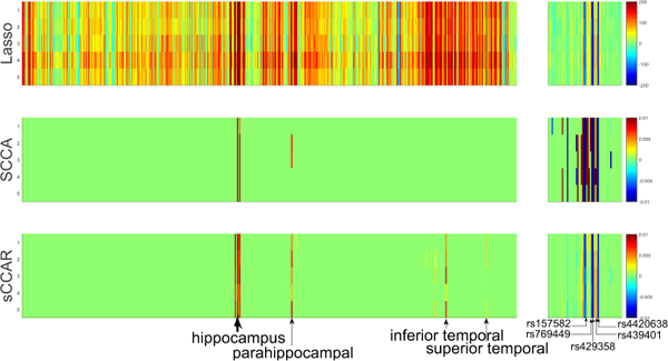
Heat maps of canonical weights on real data. Each row corresponds to a method: (1) Lasso; (2) SCCA; (3) sCCAR. Within each row, the left panel shows the weight for QTs, and the right one shows the weight for SNPs.

4. CONCLUSIONS

We proposed a novel integrated modeling method via combining CCA and regression to assure a diagnosis status guided bi-multivariate analysis tool. sCCAR outperformed SCCA and Lasso on both synthetic and real neuroimaging data. sCCAR can not only obtain better correlation coefficients, but also identify superior canonical weight pattern which indicates better feature selection ability. The results demonstrated that sCCAR could be an interesting bi- multivariate analysis method for brain imaging genetics.

References

- [1].Saykin Andrew J, Shen Li, Yao Xiaohui, Kim Sungeun, Nho Kwangsik, et al. , “Genetic studies of quantitative mci and ad phenotypes in adni: Progress, opportunities, and plans,” Alzheimer’s & Dementia, vol. 11, no. 7, pp. 792–814, 2015. [DOI] [PMC free article] [PubMed] [Google Scholar]
- [2].Shen Li, Kim Sungeun, Risacher Shannon L, Nho Kwangsik, Swaminathan Shanker, West John D, Foroud Tatiana, Pankratz Nathan, Moore Jason H, Sloan Chantel D, et al. , “Whole genome association study of brain-wide imaging phenotypes for identifying quantitative trait loci in MCI and AD: A study of the ADNI cohort,” Neuroimage, vol. 53, no. 3, pp. 1051–63, 2010. [DOI] [PMC free article] [PubMed] [Google Scholar]
- [3].Parkhomenko Elena, Tritchler David, and Beyene Joseph, “Sparse canonical correlation analysis with application to genomic data integration,” Statistical applications in genetics and molecular biology, vol. 8, no. 1, pp. 1–34, 2009. [DOI] [PubMed] [Google Scholar]
- [4].Witten DM, Tibshirani R, and Hastie T, “A penalized matrix decomposition, with applications to sparse principal components and canonical correlation analysis,” Biostatistics, vol. 10, no. 3, pp. 515–34, 2009. [DOI] [PMC free article] [PubMed] [Google Scholar]
- [5].Du Lei, Huang Heng, Yan Jingwen, Kim Sungeun, Risacher Shannon L, et al. , “Structured sparse canonical correlation analysis for brain imaging genetics: An improved graphnet method,” Bioinformatics, vol. 32, no. 10, pp. 1544–1551,2016. [DOI] [PMC free article] [PubMed] [Google Scholar]
- [6].Du Lei, Liu Kefei, Zhang Tuo, Yao Xiaohui, Yan Jingwen, Risacher Shannon L, Han Junwei, Guo Lei, Saykin Andrew J, and Shen Li, “A novel SCCA approach via truncated l1-norm and truncated group lasso for brain imaging genetics,” Bioinformatics, vol. 34, no. 2, pp. 278–285, 2018. [DOI] [PMC free article] [PubMed] [Google Scholar]
- [7].Wang Hua, Nie Feiping, Huang Heng, Kim Sungeun, Nho Kwangsik, Risacher Shannon L, Saykin Andrew J, Shen Li, et al. , “Identifying quantitative trait loci via group-sparse multitask regression and feature selection: an imaging genetics study of the ADNI cohort,” Bioinformatics, vol. 28, no. 2, pp. 229–237, 2012. [DOI] [PMC free article] [PubMed] [Google Scholar]
- [8].Tibshirani Robert, “Regression shrinkage and selection via the lasso,” Journal of the Royal Statistical Society, vol. 58, no. 1, pp. 267–288, 1996. [Google Scholar]
- [9].Dudoit Sandrine, Fridlyand Jane, and Speed Terence P, “Comparison of discrimination methods for the classification of tumors using gene expression data,” Journal of the American Statistical Association, vol. 97, no. 457, pp. 77–87, 2002. [Google Scholar]
- [10].Tibshirani Robert, Hastie T, Narasimhan Balasubramanian, and Chu Gilbert, “Class prediction by nearest shrunken centroids with application to dna microarrays,” Statistical Science, vol. 18, no. 1, pp. 104–117, 2003. [Google Scholar]
- [11].Friedman Jerome H, Hastie Trevor, Hofling Holger, and Tibshirani Robert, “Pathwise coordinate optimization,” The Annals of Applied Statistics, vol. 1, no. 2, pp. 302–332, 2007. [Google Scholar]
- [12].Hampel Harald, Burger Katharina, Teipel Stefan J, Bokde Arun LW, Zetterberg Henrik, and Blennow Kaj, “Core candidate neurochemical and imaging biomarkers of alzheimer’s disease,” Alzheimer’s & Dementia, vol. 4, no. 1, pp. 38–48, 2008. [DOI] [PubMed] [Google Scholar]