Abstract
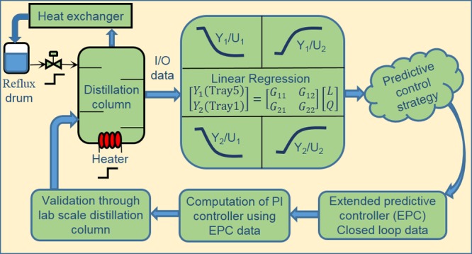
The present study proposes a new PI controller tuning method using extended predictive control (EPC). The PI controller parameter values are calculated using the EPC controller output and its closed-loop response. This provides a simple and an effective tuning strategy which results in an improved closed-loop response compared to conventional tuning methods. The tuning methodology is applicable for single input single output and multi input multi output stable processes. Simulation and experimental results reveal the efficacy of the method under plant uncertainty conditions.
1. Introduction
The three term control (PID) has been one of the simplest and most popular control approaches over six decades. The major demand of PID is due to its simple structure, ease of use, and robustness.1 Apart from a conventional structure, the control loops are modified in many ways in order to obtain better performance and efficiency.2,3 The drawback of the traditional PID controller is that it cannot handle constraints, it cannot manage strong interactions, and it is generally used in the control of simple processes.4 Therefore, off-the-shelf algorithms are not an optimal choice in many processes.5 This limitation has extended research toward advanced control areas like optimal, robust, and adaptive control.6−8 The recent developments comprise event-triggered control that deals with the problems of finite communication for constrained nonlinear systems through optimal policy.9 Model predictive control (MPC) is another control approach, which is able to handle the process interactions and constraints. It is a popular and widely used control approach in several contexts.10
MPC predicts future values of the process outputs based on a reasonably accurate dynamic model and provides the appropriate input signals by solving an optimization problem involving the computation of the optimum set points with constraints on inputs and outputs.11 Garriga and Soroush,12 presented a brief survey on various methods of control tuning in theoretical and practical aspects. Depending on applications and requirements, there exist different types of MPC algorithms like adaptive,13 explicit,14 robust,15 economic,16,17 stochastic,18 distributed,19 and so forth. Though MPC is advanced and embraces a predictive functionality, it lacks in the ease of industrial applications because of complex calculations within the sampling interval. This limitation laid the foundation toward the bridging of MPC and PID control schemes20−23 through which MPC controller gain or closed-loop data is used to tune the PID parameters. As far as industrial implementation is concerned, the idea of bridging the advanced control mechanism and conventional controller spreads over in different aspects.24 Preitl et al.25 presented two iterative control schemes to formulate an objective function and validated with a PI controller. Vrkalovic et al.26 had developed a model free sliding mode and PI-fuzzy controller using a Grey Wolf Optimizer.27 In application toward optimization techniques, the teaching–learning-based optimization algorithm is applied to obtain the parameters of the fuzzy-PID controller.28
The method proposed here is a new PI controller tuning scheme using the closed-loop data of the extended predictive control (EPC) strategy. The controller parameters are obtained as a function of EPC manipulated variable response, time constant of the actual process, rise time of EPC unit step response, and condition number “r2”. In addition to the proposed control method, the mathematical modeling presented by Fedele38 has been extended to multi input multi output (MIMO) processes. This paper is organized as follows: Section 2 presents a system description of the lab-scale distillation column and methodology of parameter estimation. The control design methodology is discussed in Section 3. Section 4 contains simulation results of parameter estimation using the procedure given in Section 2 and control scheme implementation on two case studies are presented with 30% plant parameter uncertainty. The last section is devoted to conclusions.
2. System Description and Mathematical Modeling
The model is assumed as the first order plus dead time (FOPDT) structure throughout the paper, and the system is assumed to be linear time-invariant at a certain operating region. The online binary distillation column is considered for this study with a feed mixture of 30% isopropyl alcohol and 70% water. The boiling point of isopropyl alcohol and water ranges as 81.5–82.5 °C29 and 99–100 °C correspondingly. The intent is to separate this mixture and obtain maximum purity of isopropyl alcohol through the distillation process. Unlike the application in this paper, there are mixtures called azeotropes, which exhibits the same boiling point throughout the distillation process.30 Alves et al.31 presented a new approach for the prediction of azeotrope formation using neural networks. Figure 1 depicts the schematic diagram of the bubble cap distillation column. The column consists of five trays placed in the ascending order from bottom to top which are equidistant to each other. A heater with 4000 kW is fitted at the bottom of the column, which is manipulated using solid state relay, and there is an opening to inject the feed into the column. A condenser is located at the top of the column, which is used to cool down the hot vapor, which in turn converts it into the liquid state. There is a reflux drum at the outlet of the condenser which is used to collect condensed liquid, and a drum at the bottom end is used to collect the purified distillate. Reflux flow rate is manipulated by using a peristaltic pump (model: EnerTech ENPD 100). The sensors and final control elements are interfaced with the PC (configuration: HP ProDesk 400 G3 SFF, 4 GB RAM and 512 GB) using the data acquisition card. The mathematical modeling and controller execution have been realized through Matlab 2018a.
Figure 1.
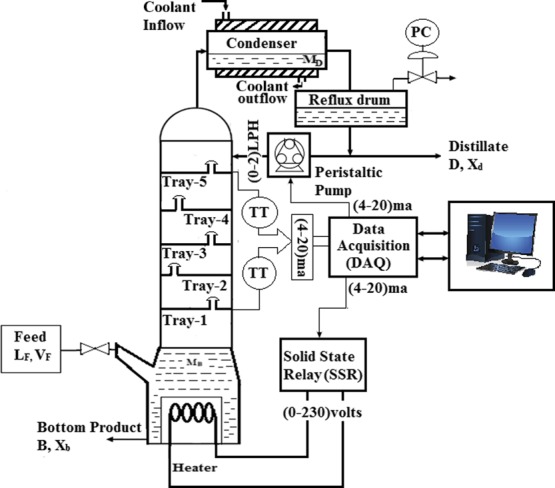
Schematic diagram of the distillation column.
Temperature control is the crucial operation of distillation which influences the purity of the distillate.32 If the temperature at a certain tray point in the system is too high or too low, expectable products or their quality may not be guaranteed.33 Controlling of such systems is a challenge because of their nonlinear behavior. The control design is more complex because of its wide operating region of feed composition and flow rates. Model identification of such systems is difficult because of interaction in the process because of tray temperatures.34,35 If the temperature at the top of the tower is more than what it should be, heavier components will be vaporized and become a part of the overhead product instead of flowing down as liquid and vice versa with lower temperatures.36 Pressure is another parameter which influences the purity of distillate through the boiling temperature of liquid.
| 1 |
For the MIMO process, the overall system equation is
 |
2 |
A linear regression approach is used to estimate system parameters through the equations that are obtained directly using the process output when the system is subjected to step change.37 Unlike other least square methods which uses the process output from t ≥ θ, this approach considers process output from time where the step change U0 is applied. The output of the process when step input is applied to eq 1 is given as
| 3 |
Differentiating eq 3 with respect to s results in
| 4 |
| 5 |
To eliminate the derivatives of laplace “s”, eq 5 is divided with s2
| 6 |
by applying inverse Laplace transform in eq 6
| 7 |
Equation 7 can be rewritten as
| 8 |
where, θT = L, g1(t) = 2∫0ty(ρ)dρ – ty(t), g2(t) = ∫0y(ρ)dρ, g3(t) = y(t), g4(t) = −∫0t∫0y(λ)dλ dρ + ∫0tρy(ρ)dρ.
The linear eq 8 allows the estimation of the unknown parameters “T” and “L” and the values of the auxiliary variable θ. To this aim, assume that gi(t), i = 1, ..., 4 are measured at times 0, Ts, ..., (n – 1)Ts, where Ts is the sampling period and “n” is the number of samples, and it is defined as
| 9 |
 |
10 |
and
 |
11 |
From eqs 9–11, eq 8 can be rewritten as
| 12 |
The estimation of parameters using least squares is obtained as
| 13 |
The system gain “K” is obtained by considering the steady state process output. Because there exist cases where the step stops before the steady state is reached, the parameter “K” has to be also identified during the plant transient response. To this aim, consider the step response of the process after t = θ.
| 14 |
Integrating y(t) from t = θ to n
| 15 |
From eq 15, process gain “K” can be obtained as
| 16 |
The mathematical modeling approach has been implemented to estimate model parameters for the lab-scale distillation column as well as Wood and Berry plant.39 Additional integral has been used in eq 7 to improve the filtering performance.
3. Control Design Methodology
A new control tuning method presented in this paper is carried out by considering the methodology of EPC and suppression matrix formulation.40 In particular, PI controller gain parameters are computed by using closed-loop data of EPC.
Extending PID controller gains from the MPC approach is a contemporary method of the advanced control theory. There exists different aspects of formulating PID gains from MPC20,41−44Table 1 reports different PID formulations based on MPC.
Table 1. Existing MPC-Based PID.
The objective function to be minimized is defined over the prediction horizon (p), as a function of error and controller response for the servo operation. This objective function is minimized by evaluating a profile of manipulated input moves implemented at every sampling instant over the control horizon (m). The control law is based on the solution of the quadratic cost function using least squares with a weighting factor on the manipulated variable.
| 17 |
In this paper, an infinite horizon control problem is considered to formulate the predictive algorithm. The unconstrained MPC control law is given by45
| 18 |
where “A” is a dynamic matrix obtained from the step response coefficients of individual transfer function (gij), where “i” is the output and “j” is the input of the process. “λ” is a suppression weighting factor, “e” is the vector of tracking difference between trajectory reference and the prediction of the process. “λI” of eq 18 is considered as the extended moving suppression matrix and it is represented as WEMS. For “n” step prediction (n = runtime), system matrix “A” of the MIMO process for “N” inputs and “M” outputs is given by
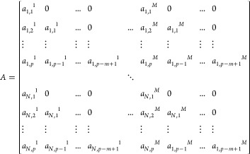 |
19 |
For the two input two output (TITO) process, eq 19 can be rewritten as
| 20 |
The weighting matrix WEMS is formulated by considering the same even elements of the first row to improve the ill conditioning of the weighting matrix. For the TITO process, WEMS is given as
| 21 |
 |
for m = 3.
The tuning parameters r1 and r2 are tuned independently based on the corresponding step response coefficient matrices A11 and A22. Initially, r2 is tuned using condition number γ through independent matrix A22. The condition number of (ATA + WEMS)−1 is obtained as
| 22 |
and approximated condition number γapprox using weighting ratio “r” and weighting factor R1 is given as
| 23 |
The analysis to formulate eqs 22 and 23 is presented by Abu-Ayyad et al.46 through a relatively lower condition number that depicts a smaller move suppression value.
The value where condition number γ and approximated condition number γapprox overlaps is considered as the tuning value of r2. Later, using r2, the tuning parameter r1 is chosen. The actual and approximated condition number comparison is shown in Figure 2. The tuning parameter R1 is considered as “10” for all processes. Another tuning parameter “β” is obtained using the initial element of matrix “ATA” from individual submatrices (A11 and A22).
Figure 2.
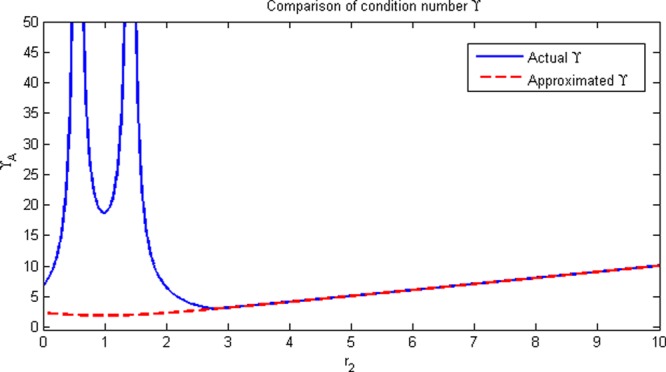
Condition number comparison of actual and approximated.
3.1. Formulation of PI Formula from EPC Control
The EPC algorithm is performed using eq 18 for unit step input in offline considering the process as an infinite prediction horizon problem (p = n). Proportional gain is computed by summing up the magnitude change of controller output “Δu” for all time samples of EPC response till its settling time. Integral gain is obtained as a function of proportional gain and rise time “Tr” of EPC unit step response.
Proportional gain
| 24 |
where “i” denotes the loop number (zth loop), δ is a tuning parameter selected as the maximum value of the off-diagonal time constant for loop-1 and the minimum value of the diagonal time constant for loop-2, that is,
“Ts” is the settling time of EPC closed-loop response and “Δu” is the change in controller output. r2 is the intersection value of the actual and approximated condition number (γ).
Integral gain
| 25 |
where “Tr” is rise time and “α” is the tuning parameter that employs the speed of the process ranging (0,1). The pace of the process is directly proportional to offline EPC response for unit step input. Tuning parameter “δ” for the single input single output (SISO) process is selected as the time constant “T” of the FOPDT model.
4. Results and Discussion
In this section, parameter estimation and validation of the control tuning method has been carried out by considering two case studies of MIMO processes. The proposed method has been compared with GPC–PID and hybrid control methods. Performance indices using integral time absolute error (ITAE) is presented with 30% uncertainty on all plant model parameters.
4.1. Parameter Estimation
The estimation of model parameters has been carried out on two case studies (case-1: Wood and Berry model39 and case-2 experimental distillation setup17). The methodology presented in Section 2 is used to estimate the model parameters.
4.1.1. Parameter Estimation Case-1: Wood and Berry Model Estimation
The Wood and Berry model is considered as the benchmark for illustrating the MIMO process. The model estimation is carried out by considering the composition of the overhead and bottom product as process variables with reflux flow and steam flow as manipulated inputs. It has been proven to be a difficult process to control because of an interaction effect between the input–output variables. The true model has been depicted in eq 26.
 |
26 |
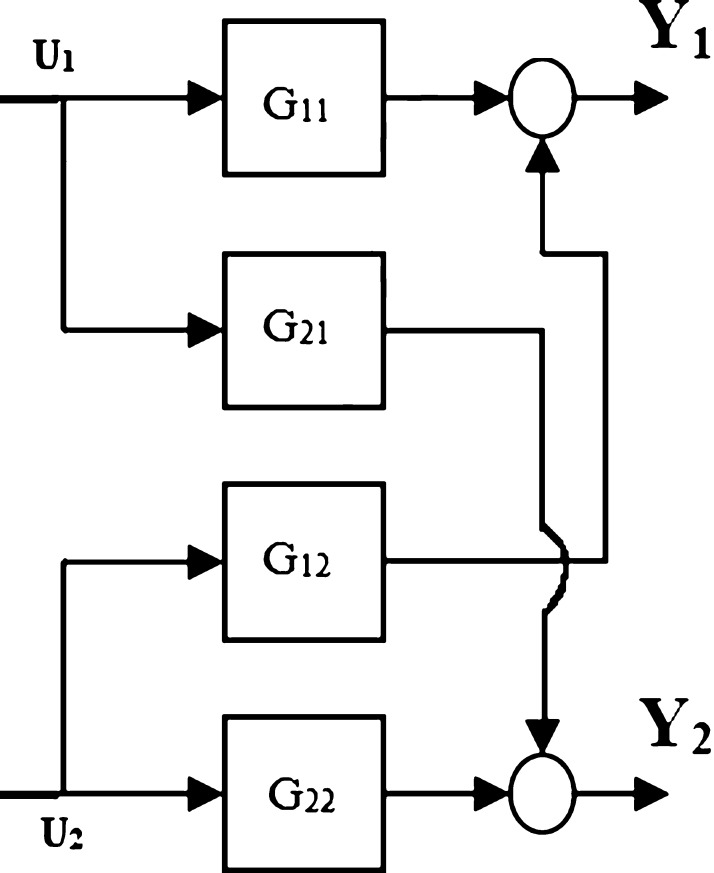
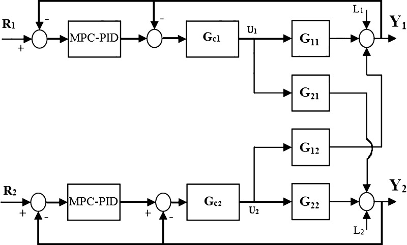
The step response data for the Wood and Berry (WB) plant is obtained by performing two experiments with unit step input sequentially for both the inputs (U1 and U2). Figure 3 depicts the block diagram of the open loop TITO process.
Figure 3.
Open loop block diagram representation for the TITO process.
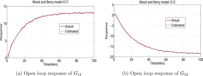
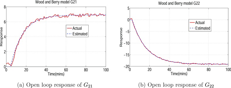
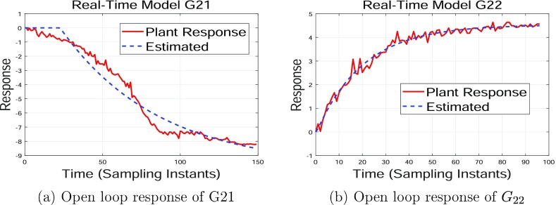
Step response data of eq 26 are used to estimate the model parameters subjected to eqs 8 and 16. Figures 4 and 5 depict fit test responses of the estimated model.
Figure 4.
G11 and G12 open loop response of the WB model.
Figure 5.
G21 and G22 open loop response of the WB model.
It is to be noted that to replicate simulation response of the WB model as actual measurement response, the plant outputs are corrupted with random Gaussian noise with zero mean and variance as a factor of 0.05 magnitude. Table 2 depicts the comparison of model parameters with absolute error and error percentage.
Table 2. Comparison of Estimated Model Parameters for the WB Model with the Actual Model.
| parameters | actual model parameters | estimated model parameters | absolute error | error (%) |
|---|---|---|---|---|
| K11 | 12.8 | 12.78 | 0.02 | 0.15 |
| T11 | 16.7 | 16.65 | 0.05 | 0.29 |
| θ11 | 1 | 1.04 | 0.04 | 4 |
| K12 | –18.9 | –18.92 | 0.02 | 0.1 |
| T12 | 21 | 21.04 | 0.04 | 0.19 |
| θ12 | 3 | 2.97 | 0.03 | 1 |
| K21 | 6.6 | 6.575 | 0.025 | 0.37 |
| T21 | 10.9 | 10.75 | 0.15 | 1.37 |
| θ21 | 7 | 7.18 | 0.18 | 2.57 |
| K22 | –19.4 | –19.42 | 0.02 | 0.1 |
| T22 | 14.4 | 14.45 | 0.05 | 0.34 |
| θ22 | 3 | 2.97 | 0.03 | 1 |
Therefore the estimated model is given as
 |
27 |
4.1.2. Parameter Estimation Case-2: Lab-Scale Distillation Column
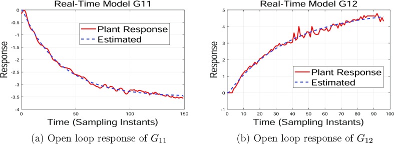
A highly interactive lab-scale distillation column (Figure 17) is considered for the experimental study to estimate the model parameters. The two tray temperatures (tray-1 and tray-5) are considered as process variables with heater voltage (Qh) and reflux flow rate (Lr) as manipulated inputs correspondingly. The step test has been performed for both the inputs sequentially by manipulating one input change at a time. Figures 6 and 7 show fit test of the lab-scale distillation column.
Figure 17.
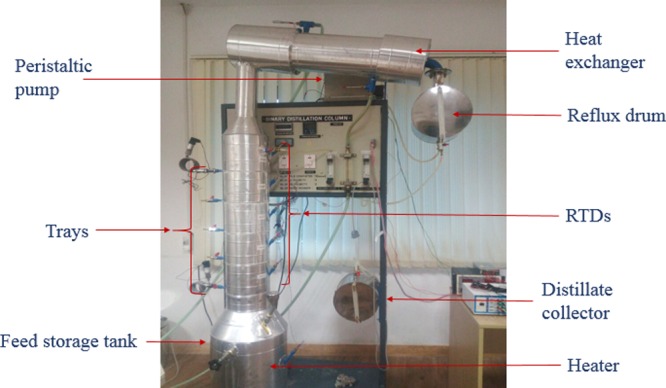
Lab-scale binary distillation column (available in lab-2, ICE dept, MIT, Manipal).
Figure 6.
G11 and G12 open loop response of the experimental system.
Figure 7.
G21 and G22 open loop response of the experimental system.
The initial manipulated input are considered as, [Lr, Qh] = [10, 50]%. For step-1, the inputs are excited from [10, 50] to [35, 50]% and corresponding response at Y1 and Y2 is observed. Similarly, for step-2, the inputs are excited from [10, 50] to [10, 75]%.
Note that because of steady state requirement, the step response time with step change in reflux flow rate is more than the step change-applied heater voltage with respect to the variable of interest.
The model estimated by using eqs 8 and 16 is
 |
28 |
4.2. Implementation of Control Schemes
The decentralized control structure with a decoupler shown in Figure 8 is considered for the simulation and comparison of the proposed controller with GPC–PID,42,47 and the hybrid control approach41 has been used. Simulation is executed with servo and regulatory operations under 30% plant parameter uncertainties in “K”, “τ”, and “θ”.
Figure 8.
Decentralized control structure with a decoupler, where, D11 = D22 = 1, D21 = −G21/G22, and D12 = −G12/G11.
4.2.1. Case Study-1: Wood and Berry Model
4.2.1.1. Servo Operation
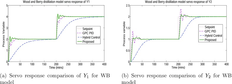
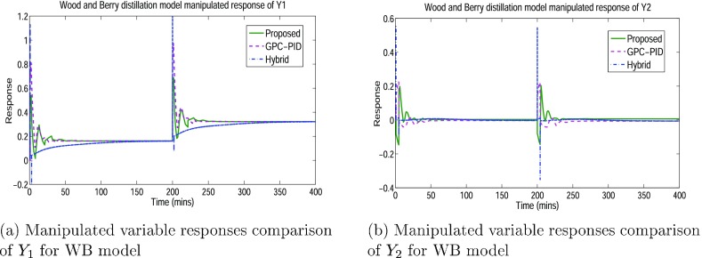
The Wood and Berry model is subjected to closed-loop simulation with set point step changes of [2,4], applied at time (0,200) min for loop-1. The response is observed at Y1, as shown in Figure 9a, and for loop-2, the response of process variable Y2 with set point step changes of [1,2], applied at time (0,200) min, is represented in Figure 9b. Correspondingly, manipulated variable responses of loop-1 and loop-2 are shown in Figure 10a,b, respectively. The controller parameters using GPC-PID and proposed methodology for Wood and Berry model is given in Table 7 and Table 8, respectively.
Figure 9.
Process variable simulation response comparison of Y1 and Y1 for the WB model.
Figure 10.
Manipulated variable response comparison of Y1 and Y2 for the WB model.
Table 7. GPC–PID Controller: Wood and Berry.
| parameters | loop-1 | loop-2 |
|---|---|---|
| KP | 0.3886 | –0.168 |
| KI | 0.0932 | –0.012 |
| KD | 0.527 | –0.161 |
Table 8. Proposed Controller: Wood and Berry.
| parameters | loop-1 | loop-2 |
|---|---|---|
| KP | 0.347 | –0.091 |
| KI | 0.0662 | –0.0212 |
4.2.1.2. Regulatory Operation
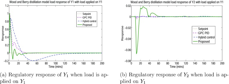
Load on both the loops are imposed individually at the zero steady state, as shown in Figure 8. When load (L1) is applied at output Y1, the effect observed on output Y1 is quoted as the main effect, and the effect observed on output Y2 is the interaction effect to the load at Y1. It is the same in the case of load (L2) on Y2 as well. Figure 11a depicts the response of Y1 when load is applied at Y1. For the same load at Y1, the response of Y2 is shown in Figure 11b.
Figure 11.
Regulatory response of Y1 and Y2 when load (d1) is applied on Y1.
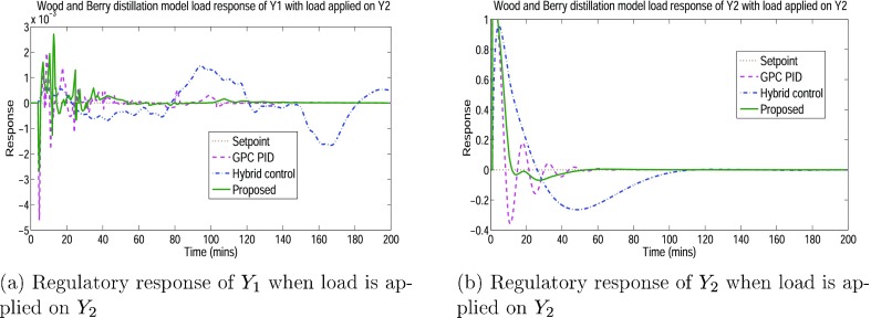
Similarly, Figure 12a depicts the response of Y1 when load is applied at Y2. For the same load at Y2, the response of Y2 is shown in Figure 12b.
Figure 12.
Regulatory response of Y1 and Y2 when load is applied on Y2.
4.2.1.3. Performance Indices
When determining the performance of the controller, it is often helpful to consider how “large” the error from the setpoint is. ITAE is one of the criteria that are used to evaluate the controller performance by essentially adding errors at every sampling instant over a period of run-time. System perturbation is one aspect of determining the efficiency of the controller. In this paper, plant parameters are perturbed with 30% uncertainty in all individual model parameters with four cases (C-1 is nominal plant; C-2 is 30% uncertainty in “K”; C-3 is 30% uncertainty in “K” and “T”; and C-4 is 30% uncertainty in “K”, “T”, and θ). Table 3 refers to servo operation performance of the Wood and Berry model with plant uncertainties for different control schemes.
Table 3. ITAE Values of the WB Model with Uncertainty (Servo Operation).
| methods | main | interaction | total | |
|---|---|---|---|---|
| C-1 | GPC–PID | 126.48 | 11.32 | 137.8 |
| hybrid | 7089 | 1.98 | 7090.98 | |
| proposed | 105.26 | 5.91 | 111.17 | |
| C-2 | GPC–PID | 416.52 | 201.7 | 618.22 |
| hybrid | 3252.4 | 460.4 | 3712.8 | |
| proposed | 191.4 | 159.82 | 350.96 | |
| C-3 | GPC–PID | 380.3 | 163.29 | 543.59 |
| hybrid | 3229.1 | 628.9 | 3858 | |
| proposed | 322.12 | 267.56 | 589.68 | |
| C-4 | GPC–PID | 388.25 | 197.19 | 585.44 |
| hybrid | 3206.2 | 614.2 | 3820.4 | |
| proposed | 291.56 | 258.02 | 549.58 |
Table 4 depicts the ITAE values of the WB model subjected to regulatory operation in comparison with different control schemes under plant uncertainties.
Table 4. ITAE Values of the WB Model with Uncertainty (Load Operation).
| methods | main | interaction | total | |
|---|---|---|---|---|
| C-1 | GPC–PID | 126.82 | 12.02 | 138.84 |
| hybrid | 942.3 | 2.29 | 944.59 | |
| proposed | 105.36 | 5.77 | 111.13 | |
| C-2 | GPC–PID | 420.4 | 210.7 | 631.1 |
| hybrid | 1600 | 1241 | 2841 | |
| proposed | 191.02 | 159.77 | 350.79 | |
| C-3 | GPC–PID | 380.4 | 162.99 | 543.39 |
| hybrid | 2221.1 | 2132.906 | 4354.006 | |
| proposed | 321.9 | 267.37 | 589.27 | |
| C-4 | GPC–PID | 386.24 | 201.69 | 587.93 |
| hybrid | 2153.2 | 1697.8 | 3851 | |
| proposed | 291.37 | 255.74 | 547.11 |
4.2.2. Case Study-2: Lab-Scale Distillation Column Model
4.2.2.1. Servo Operation
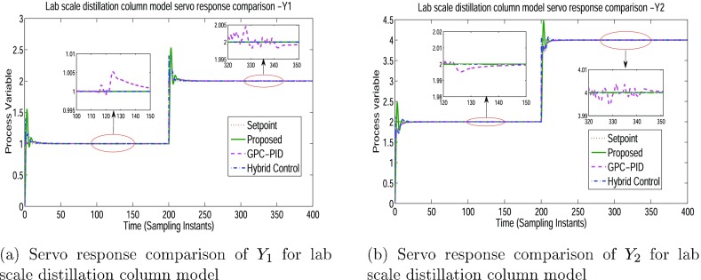
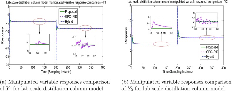
Lab-scale plant model 27 is subjected to closed-loop simulation with set point step changes of (1,2) applied at time (0,200) min for loop-1. The response is observed at Y1 as shown in Figure 13a. Similarly, for loop-2, set point step changes of (2,4) is applied at time (0,200) min and the response is observed at Y2 depicted in Figure 13b. Manipulated variable response of loop-1 and loop-2 is given in Figure 14a,b respectively. The controller parameters using GPC-PID and proposed methodology for pilot-Scale Distillation Column Model is given in Table 9 and Table 10, respectively.
Figure 13.
Process variable responses of Y1 and Y2 for the lab-scale distillation column.
Figure 14.
Manipulated variable responses of Y1 and Y2 for the lab-scale distillation column.
Table 9. GPC–PID Controller: Pilot-Scale Distillation Column.
| parameters | loop-1 | loop-2 |
|---|---|---|
| KP | –8.02 | 3.67 |
| KI | –0.937 | 1.198 |
| KD | –2.574 | 3.943 |
Table 10. Proposed Controller: Pilot-Scale Distillation Column.
| parameters | loop-1 | loop-2 |
|---|---|---|
| KP | –1.1056 | 0.6879 |
| KI | –0.9641 | 1.7533 |
4.2.2.2. Regulatory Operation
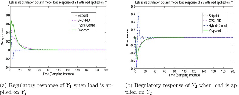
The load on both the loops is imposed individually on the initial state of system at zeroth sampling instant. Figure 15a depicts the response of Y1 when load is applied at Y1. For the same load at Y1, the response of Y2 is shown in Figure 15b.
Figure 15.
Regulatory response of Y1 and Y2 when load is applied on Y1 (pilot plant model).
Similarly, Figure 16a depicts the response of Y1 when load is applied at Y2. For the same load at Y2, the response of Y2 is shown in Figure 16b.
Figure 16.
Regulatory response of Y1 and Y2 when load is applied on Y2 (pilot plant model).
4.2.2.3. Performance Indices
Table 5 refers to ITAE values of servo operation of the pilot-scale plant model with plant uncertainties in comparison with different control schemes. Table 6 depicts the ITAE values of the pilot-scale plant model subjected to regulatory operation in comparison with different control schemes under plant uncertainties.
Table 5. ITAE Values of the Pilot Plant Model with Uncertainty (Servo Operation).
| methods | main | interaction | total | |
|---|---|---|---|---|
| C-1 | GPC–PID | 146.45 | 125.17 | 271.62 |
| hybrid | 60.28 | 59.78 | 120.06 | |
| proposed | 60.78 | 53.64 | 114.42 | |
| C-2 | GPC–PID | 156.07 | 143.07 | 299.14 |
| hybrid | 66.47 | 65.86 | 132.33 | |
| proposed | 63.99 | 61.33 | 125.32 | |
| C-3 | GPC–PID | 152.02 | 139.4 | 291.42 |
| hybrid | 77.04 | 82.41 | 159.45 | |
| proposed | 60.02 | 57.75 | 117.77 | |
| C-4 | GPC–PID | 152.6 | 139.96 | 292.56 |
| hybrid | 64.15 | 68.98 | 133.53 | |
| proposed | 60.55 | 58.21 | 118.76 |
Table 6. ITAE Values of the Pilot Plant Model with Uncertainty (Load Operation).
| methods | main | interaction | total | |
|---|---|---|---|---|
| C-1 | GPC–PID | 157.42 | 134.94 | 291.91 |
| hybrid | 40 | 40 | 80 | |
| proposed | 70.61 | 61.42 | 132.03 | |
| C-2 | GPC–PID | 168.49 | 154.32 | 322.91 |
| hybrid | 50.82 | 50.66 | 101.48 | |
| proposed | 74.14 | 69.85 | 143.99 | |
| C-3 | GPC–PID | 163.72 | 149.83 | 313.57 |
| hybrid | 79.6 | 81.55 | 161.15 | |
| proposed | 70.19 | 66.32 | 136.51 | |
| C-4 | GPC–PID | 164.39 | 150.42 | 314.81 |
| hybrid | 70.65 | 73.83 | 144.48 | |
| proposed | 70.64 | 66.7 | 137.34 |
Overall performance of hybrid control is efficient compared to the proposed algorithm in case of nominal and uncertainty in “K” but lags when uncertainty is introduced in “T” and θ cases. Through the performance index, it has been observed that the proposed control scheme is effective compared to GPC–PID and hybrid control schemes.
5. Conclusions
In this work, the parameter estimation using the regression method has been carried out, and the obtained model is in the form of the FOPDT structure. The development of a new PI control tuning approach has been presented from the EPC strategy. The controller parameters are formulated from summation of instantaneous controller changes and rise time of the closed-loop unit step response of EPC. The application of this novel design has been demonstrated through benchmark and experimental models of the distillation process. Performance analysis has been carried out to depict the efficiency of the controller under plant uncertainty and compared with other well-accepted control schemes.
6. Experimental Implementation and Analysis
The proposed controller has been implemented on the experimental setup shown in Figure 17 to control coupled tray temperature.
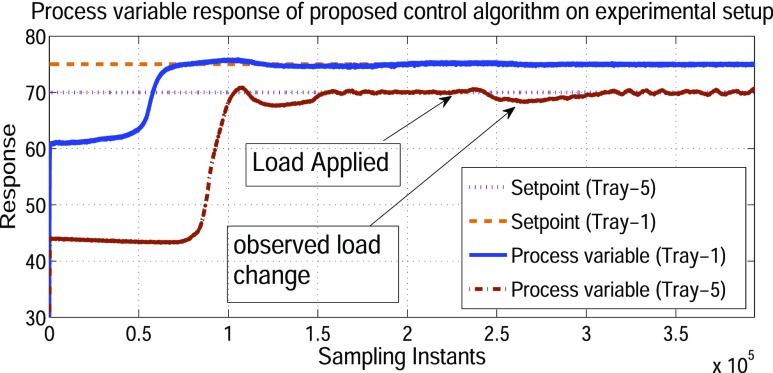
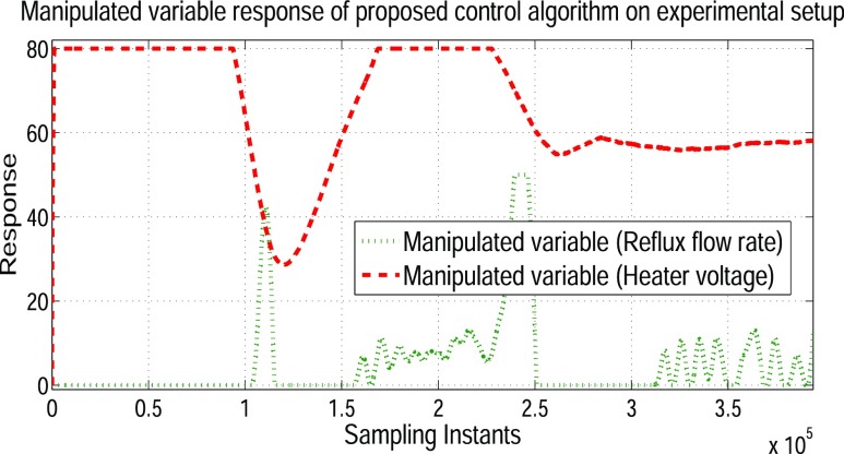
Figures 18 and 19 depict process variables and manipulated variable response of the lab-scale distillation column. The operating region of tray temperature was initialized at [61, 44] °C and the proposed controller was implemented with set points of [75, 70] °C for tray-1 and tray-5, respectively. As the system reached the desired state, the pressure valve on the reflux drum is disturbed to observe the regulatory operation. In rejecting the load disturbance, the controller effect has been observed on both the manipulated inputs.
Figure 18.
Experimental response of process variables for the proposed controller.
Figure 19.
Experimental response of manipulated variables for the proposed controller.
There is an arrangement of the pressure knob on the reflux drum which is used to release excess pressure in the column. The system is perturbed with an external disturbance by releasing pressure manually using the pressure knob, and the regulatory response effecting temperature of tray-5 is observed. When the disturbance is applied at 2.25 × 10⁴ sampling instant, the effect of the load is observed at 2.65 × 10⁴ sampling instant (because temperature control is a slow process). While controlling tray temperature, the controller tends toward saturation because of integral windup. To overcome integral windup, a conditional integrator approach3 is used within the control loop.
Acknowledgments
The first author would like to acknowledge the Manipal Academy of Higher Education for providing stipend under TMA Pai scholarship toward this experimental research work. The authors would like to thank the department of Instrumentation and Control Engineering, Manipal Institute of Technology, for providing the experimental facility. Our special thanks to Dr. J. Prakash, Anna University, Tamilnadu, India, for timely suggestions and guidance in this work. We would also like to thank Dr. R. Russell Rhinehart, Professor Emeritus, Chemical Engineering, Oklahoma State University, Stillwater, USA, for the technical inputs to improve the paper.
Glossary
Nomenclature
- θ
dead time
- C-1
nominal plant
- C-2
uncertainty in “K”
- C-3
uncertainty in “K” and “T”
- C-4
uncertainty in “K”, “T”, and “θ”
- EPC
extended predictive control
- GPC
generalized predictive control
- IO
input–output
- ITAE
integral time absolute error
- K
process gain
- Lr
reflux flow rate
- m
control horizon
- MIMO
multi input multi output
- MPC
model predictive control
- n
total run-time
- p
prediction horizon
- PID
proportional integral and derivative
- PSDC
pilot-scale distillation column
- Qh
heater voltage
- SISO
single input single output
- T
time constant
- Ts
sampling interval
- TITO
two input two output
- TT
temperature transmitter
- WB
Wood and Berry
- Xb
bottom product concentration (mol/h)
- Xd
distillate concentration (mol/h)
Appendix
Wood and Berry decoupler model
 |
Pilot-scale distillation column decoupler model
 |
Controller Gain Parameters
The authors declare no competing financial interest.
References
- Åström K. J.; Hägglund T.. Advanced PID Control; ISA-The Instrumentation, Systems, and Automation Society Research Triangle, 2006; pp 1–10. [Google Scholar]
- Majhi S.; Atherton D. P. Modified Smith predictor and controller for processes with time delay. IEE Proc. Control Theory Appl. 1999, 146, 359–366. 10.1049/ip-cta:19990502. [DOI] [Google Scholar]
- Visioli A.Practical PID Control; Springer Science & Business Media, 2006; pp 1–18. [Google Scholar]
- García C. E.; Prett D. M.; Morari M. Model predictive control: theory and practiceâĂŤa survey. Automatica 1989, 25, 335–348. 10.1016/0005-1098(89)90002-2. [DOI] [Google Scholar]
- Sung S. W.; Lee I.-B. Limitations and countermeasures of PID controllers. Ind. Eng. Chem. Res. 1996, 35, 2596–2610. 10.1021/ie960090+. [DOI] [Google Scholar]
- Bielecki T. R.; Chen T.; Cialenco I.; Cousin A.; Jeanblanc M. Adaptive robust control under model uncertainty. SIAM J. Control Optim. 2019, 57, 925–946. 10.1137/17m1137917. [DOI] [Google Scholar]
- Liu G. P.; Daley S. Optimal-tuning PID control for industrial systems. Contr. Eng. Pract. 2001, 9, 1185–1194. 10.1016/s0967-0661(01)00064-8. [DOI] [Google Scholar]
- Ioannou P. A.; Sun J.. Robust Adaptive Control; Courier Corporation, 2012; pp 5–23. [Google Scholar]
- Zhu Y.; Zhao D.; He H.; Ji J. Event-triggered optimal control for partially unknown constrained-input systems via adaptive dynamic programming. IEEE Trans. Ind. Electron. 2016, 64, 4101–4109. 10.1109/tie.2016.2597763. [DOI] [Google Scholar]
- Rawlings J. B.; Mayne D. Q.. Model Predictive Control: Theory and Design; Nob Hill Pub: Madison, Wisconsin, 2009; pp 1–60. [Google Scholar]
- Qin S. J.; Badgwell T. A. A survey of industrial model predictive control technology. Contr. Eng. Pract. 2003, 11, 733–764. 10.1016/s0967-0661(02)00186-7. [DOI] [Google Scholar]
- Garriga J. L.; Soroush M. Model predictive control tuning methods: A review. Ind. Eng. Chem. Res. 2010, 49, 3505–3515. 10.1021/ie900323c. [DOI] [Google Scholar]
- Adetola V.; DeHaan D.; Guay M. Adaptive model predictive control for constrained nonlinear systems. Syst. Control Lett. 2009, 58, 320–326. 10.1016/j.sysconle.2008.12.002. [DOI] [Google Scholar]
- Tøndel P.; Johansen T. A.; Bemporad A. An algorithm for multi-parametric quadratic programming and explicit MPC solutions. Automatica 2003, 39, 489–497. 10.1016/s0005-1098(02)00250-9. [DOI] [Google Scholar]
- Pluymers B.; Rossiter J. A.; Suykens J. A. K.; De Moor B. A simple algorithm for robust MPC. IFAC Proc. Vol. 2005, 38, 257–262. 10.3182/20050703-6-cz-1902.00987. [DOI] [Google Scholar]
- Touretzky C. R.; Baldea M. Integrating scheduling and control for economic MPC of buildings with energy storage. J. Process Control 2014, 24, 1292–1300. 10.1016/j.jprocont.2014.04.015. [DOI] [Google Scholar]
- Hovgaard T. G.; Edlund K.; Jørgensen J. B.. The potential of economic MPC for power management. 49th IEEE Conference on Decision and Control (CDC), 2010; pp 7533–7538.
- Di Cairano S.; Bernardini D.; Bemporad A.; Kolmanovsky I. V. Stochastic MPC with learning for driver-predictive vehicle control and its application to HEV energy management. IEEE Trans. Control Syst. Technol. 2013, 22, 1018–1031. 10.1109/tcst.2013.2272179. [DOI] [Google Scholar]
- Alvarado I.; Limon D.; Muñoz de la Peña D.; Maestre J. M.; Ridao M. A.; Scheu H.; Marquardt W.; Negenborn R. R.; De Schutter B.; Valencia F.; et al. A comparative analysis of distributed MPC techniques applied to the HD-MPC four-tank benchmark. J. Process Control 2011, 21, 800–815. 10.1016/j.jprocont.2011.03.003. [DOI] [Google Scholar]
- Tan K. K.; Lee T. H.; Huang S. N.; Leu F. M. PID control design based on a GPC approach. Ind. Eng. Chem. Res. 2002, 41, 2013–2022. 10.1021/ie010480i. [DOI] [Google Scholar]
- Camacho E. F.; Bordons C.. Model Predictive Control; Springer London, 2007; pp 81–125. [Google Scholar]
- Sarath Yadav E.; Indiran T. PRBS based model identification and GPC PID control design for MIMO Process. Mater. Today: Proc. 2019, 17, 16–25. 10.1016/j.matpr.2019.06.396. [DOI] [Google Scholar]
- Kouvaritakis B.; Cannon M.. Model Predictive Control; Springer International Publishing: Switzerland, 2016; pp 1–62. [Google Scholar]
- Åström K. J.; Hägglund T. The future of PID control. Contr. Eng. Pract. 2001, 9, 1163–1175. 10.1016/s0967-0661(01)00062-4. [DOI] [Google Scholar]
- Preitl S.; Precup R.-E.; Preitl Z.; Vaivoda S.; Kilyeni S.; Tar J. K. Iterative Feedback and Learning Control. Servo systems applications. IFAC Proc. Vol. 2007, 40, 16–27. 10.3182/20070709-3-ro-4910.00004. [DOI] [Google Scholar]
- Vrkalovic S.; Lunca E.-C.; Borlea I.-D. Model-free sliding mode and fuzzy controllers for reverse osmosis desalination plants. Int. J. Artif. Intell. 2018, 16, 208–222. [Google Scholar]
- Rathore N. S.; Singh V. P.; Kumar B. Controller design for doha water treatment plant using grey wolf optimization. J. Intell. Fuzzy Syst. 2018, 35, 5329–5336. 10.3233/jifs-169815. [DOI] [Google Scholar]
- Sahu B. K.; Pati S.; Mohanty P. K.; Panda S. Teaching–learning based optimization algorithm based fuzzy-PID controller for automatic generation control of multi-area power system. Appl. Soft Comput. 2015, 27, 240–249. 10.1016/j.asoc.2014.11.027. [DOI] [Google Scholar]
- Seth S.; Agrawal Y. C.; Ghosh P. K.; Jayas D. S.; Singh B. P. N. Oil extraction rates of soya bean using isopropyl alcohol as solvent. Biosyst. Eng. 2007, 97, 209–217. 10.1016/j.biosystemseng.2007.03.008. [DOI] [Google Scholar]
- Ewell R. H.; Harrison J. M.; Berg L. Azeotropic distillation. Ind. Eng. Chem. 1944, 36, 871–875. 10.1021/ie50418a002. [DOI] [Google Scholar]
- Alves R. M. B.; Quina F. H.; Nascimento C. A. O. New approach for the prediction of azeotropy in binary systems. Comput. Chem. Eng. 2003, 27, 1755–1759. 10.1016/s0098-1354(03)00150-9. [DOI] [Google Scholar]
- Ogunnaike B. A.; Ray W. H.. Process Dynamics, Modeling, and Control; Oxford University Press: New York, 1994; Vol. 1, pp 1–54. [Google Scholar]
- Skogestad S. Dynamics and Control of Distillation Columns - A Critical Survey. Model. Identif. Control 1997, 18, 177–217. 10.4173/mic.1997.3.1. [DOI] [Google Scholar]
- Martin P. A.; Odloak D.; Kassab F. Robust model predictive control of a pilot plant distillation column. Contr. Eng. Pract. 2013, 21, 231–241. 10.1016/j.conengprac.2012.10.004. [DOI] [Google Scholar]
- Mansouri S. S.; Huusom J. K.; Gani R.; Sales-Cruz M. Systematic integrated process design and control of binary element reactive distillation processes. AIChE J. 2016, 62, 3137–3154. 10.1002/aic.15322. [DOI] [Google Scholar]
- Andersen H. W.; Kümmel M.; Jørgensen S. B. Dynamics and identification of a binary distillation column. Chem. Eng. Sci. 1989, 44, 2571–2581. 10.1016/0009-2509(89)85201-7. [DOI] [Google Scholar]
- Eisinberg A.; Fedele G.; Frascino D.. An analytic optimization procedure to estimate a first-order plus time delay model from step response. 2008 16th Mediterranean Conference on Control and Automation, 2008; pp 729–734.
- Fedele G. A new method to estimate a first-order plus time delay model from step response. J. Franklin Inst. 2009, 346, 1–9. 10.1016/j.jfranklin.2008.05.004. [DOI] [Google Scholar]
- Wood R. K.; Berry M. W. Terminal composition control of a binary distillation column. Chem. Eng. Sci. 1973, 28, 1707–1717. 10.1016/0009-2509(73)80025-9. [DOI] [Google Scholar]
- Abu-Ayyad M.; Dubay R. MIMO extended predictive control-implementation and robust stability analysis. ISA Trans. 2006, 45, 545–561. 10.1016/s0019-0578(07)60231-6. [DOI] [PubMed] [Google Scholar]
- Yuan H.-B.; Na H.-C.; Kim Y.-B. Robust MPC–PIC force control for an electro-hydraulic servo system with pure compressive elastic load. Contr. Eng. Pract. 2018, 79, 170–184. 10.1016/j.conengprac.2018.07.009. [DOI] [Google Scholar]
- Johnson M. A.; Moradi M. H.. PID Control; Springer, 2005; pp 473–515. [Google Scholar]
- Abdelrauf A. A.; Abdel-Geliel M.; Zakzouk E.. Adaptive PID controller based on model predictive control. 2016 European Control Conference (ECC), 2016; pp 746–751.
- Sato T.; Inoue A.; Yamamoto T. Improvement of tracking performance in designing a GPC-based PID controller using a time-varying proportional gain. IEEJ Trans. Electr. Electron. Eng. 2006, 1, 438–441. 10.1002/tee.20085. [DOI] [Google Scholar]
- Shridhar R.; Cooper D. J. A tuning strategy for unconstrained SISO model predictive control. Ind. Eng. Chem. Res. 1997, 36, 729–746. 10.1021/ie9604280. [DOI] [Google Scholar]
- Abu-Ayyad M.; Dubay R.; Kember G. C. SISO extended predictive control formulation and the basic algorithm. ISA Trans. 2006, 45, 9–20. 10.1016/s0019-0578(07)60061-5. [DOI] [PubMed] [Google Scholar]
- Saeed Q.; Uddin V.; Katebi R. Multivariable predictive PID control for quadruple tank. World Acad. Sci. Eng. Technol. 2010, 4, 861–866. [Google Scholar]


