A Deep Learning Approach for Meibomian Gland Atrophy Evaluation in Meibography Images

Abstract

Purpose

To develop a deep learning approach to digitally segmenting meibomian gland atrophy area and computing percent atrophy in meibography images.

Methods

A total of 706 meibography images with corresponding meiboscores were collected and annotated for each one with eyelid and atrophy regions. The dataset was then divided into the development and evaluation sets. The development set was used to train and tune the deep learning model, while the evaluation set was used to evaluate the performance of the model.

Results

Four hundred ninety-seven meibography images were used for training and tuning the deep learning model while the remaining 209 images were used for evaluations. The algorithm achieves 95.6% meiboscore grading accuracy on average, largely outperforming the lead clinical investigator (LCI) by 16.0% and the clinical team by 40.6%. Our algorithm also achieves 97.6% and 95.4% accuracy for eyelid and atrophy segmentations, respectively, as well as 95.5% and 66.7% mean intersection over union accuracies (mean IU), respectively. The average root-mean-square deviation (RMSD) of the percent atrophy prediction is 6.7%.

Conclusions

The proposed deep learning approach can automatically segment the total eyelid and meibomian gland atrophy regions, as well as compute percent atrophy with high accuracy and consistency. This provides quantitative information of the gland atrophy severity based on meibography images.

Translational Relevance

Based on deep neural networks, the study presents an accurate and consistent gland atrophy evaluation method for meibography images, and may contribute to improved understanding of meibomian gland dysfunction.

Introduction

Dry eye disease is a multifactorial ocular surface disorder and is very common among adults. Meibomian glands (MGs) are believed to play a critical role in ocular surface health by secreting lipids into the tear film to slow down the rate of aqueous evaporation and minimize symptoms of dry eye. Dysfunction of MGs is the most frequent cause of dry eyes.1 The ability to visualize the glands and to monitor their changes with time or treatment is important for evaluating the risk of meibomian gland dysfunction (MGD) and dry eye diseases. Meibography, which is a photo documentation of MGs in the eyelids using either transillumination or infrared light, is commonly used in dry eye clinics for the diagnosis, treatment, and management of MGD.

The measurement of glandular loss is of significant clinical impact for the diagnosis of MGD.2,3 Percent MG atrophy, the ratio of gland loss area to the total eyelid area, may be an important clinical factor for assessing MGD severity. Using a standardized MG atrophy grading scale, the percent atrophy can be classified based on severity.4,5 In this paper, a previously published clinical-grading system6 (i.e., meiboscore) was applied (Table 1). Figure 1 depicts some sample meibography images with varying percent atrophy and corresponding meiboscores to help readers gain insights on the relationship between the percent atrophy and meiboscore. Currently, clinicians subjectively estimate the degree of MG atrophy severity. They assign a severity score after grossly estimating the relative ratio between MG atrophy area and total eyelid area. This subjective assessment has several limitations: (1) it may have high inter- and intraobserver variability and low repeatability7,8; (2) it is based on qualitative judgments, therefore lacking quantitative evaluations to accurately track longitudinal changes; and (3) it may take a longer time and more costs to manually process a large number of images.

Table 1.

Percent MG Atrophy to Meiboscore Conversion Criteria6

MG Atrophy, %	Meiboscore
0	0
0–33	1
33–66	2
>66	3

Figure 1.

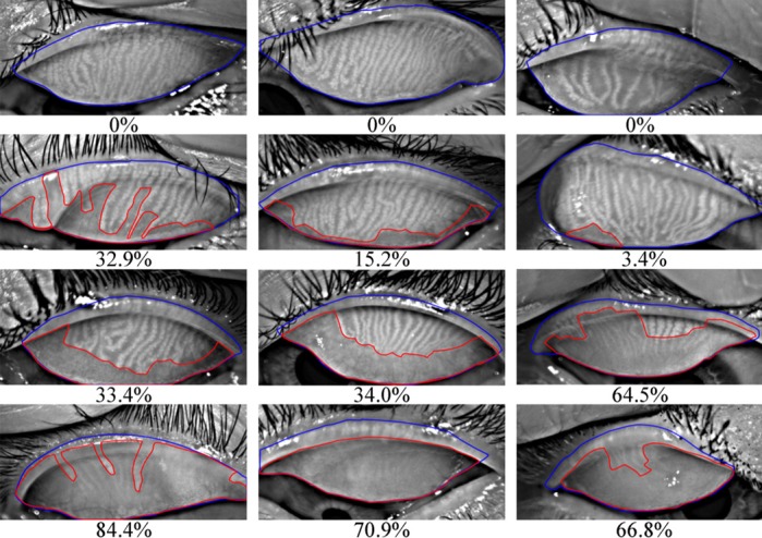
Meibography images with ground-truth percent atrophies (%) and ground-truth meiboscores. Rows 1 to 4 refer to images with meiboscores of grade 0 to 3, respectively. Given a meibography image, the area of gland atrophy (marked in red) and eyelid (marked in blue) are compared by our deep learning algorithm to estimate the percent atrophy (Equation 1), and are further converted to meiboscore according to the criteria in Table 1.

Recent advances in deep learning,9–11 a particular form of artificial intelligence (AI), show the ability of deep neural networks to learn predictive features directly from a large dataset of labeled images, without explicitly specifying rules or features. Additionally, deep learning has shown great success in medical imaging, such as diabetic retinopathy,12–14 breast cancer,15,16 melanoma,17 and others.18,19 It is of interest to use deep learning methods to benefit the process of evaluating atrophy in meibography images. Specifically, clinicians can use such methods to automatically segment the eyelid and atrophy areas in meibography images, and then compute the percent atrophy, for the purpose of evaluating MG atrophy. Therefore, an automated method will potentially provide valuable and timely information on MG atrophy.

This study aimed primarily to develop and validate an automated deep learning system for evaluating MG atrophy severity from meibography images with clinician-verified annotations of eyelid and atrophy areas. Additionally, the performance of human clinicians and deep learning algorithm in determining the atrophy severity in meibography images were compared.

Methods

Development and Evaluation Dataset

This study was based on the utilization of a meibography image dataset with clinician-verified annotations of eyelid and atrophy areas, for deep learning algorithm development and evaluation.

Subject Recruitment and Demographics

Adult human subjects (ages ≥18 years) were recruited from the University of California, Berkeley (UCB) campus and surrounding community for a single-visit ocular surface evaluation during the period from 2012 to 2017. During the visits, meibography images of the upper and lower eyelids for both eyes were captured with the OCULUS Keratograph 5M (OCULUS, Arlington, WA), a clinical instrument that uses an infrared light with wavelength 880 nm for MG imaging.20 During image captures, the same testing conditions were kept (i.e., the ambient light was off with the subject's head positioned on the chin rest and forehead strap). Yeh and Lin21 showed that MG contrast in meibography captured using the same instrument was repeatable and invariant to ambient light conditions and head poses. Only upper eyelid images were used in this study. A total of 775 images were collected and prescreened to rule out images that did not capture the entire upper eyelid (69 images or 8.90%). Examining clinicians assigned an MG atrophy severity score during the exam using the meiboscore scale in Table 1, which was previously defined.6 The meiboscores assigned during the examination were referred to as “clinical meiboscore” and were assigned by multiple clinicians. All clinicians were masked from the subject's ocular surface health status. The most experienced clinician (TNY) also provided a separate set of the clinical meiboscore data for evaluation purposes (i.e., comparing scores among group clinicians, the lead clinical investigator [LCI] and our machine-learning algorithm against the ground-truth data generated by the machine algorithms). Subject demographics can be found in Table 2.

Table 2.

Subject Demographics and Meiboscores of the Meibography Image Datasets

	Development		Evaluation
	Train	Validation
Images, N	398	99	209
Patient demographics
Unique individuals, N	308	77	191
Age, average ± SD	25.5 ± 10.9	27.0 ± 12.6	26.4 ± 11.6
Female/total patients, %	63.5	66.6	68.3
Atrophy severity distribution, n (%)
Meiboscore 0	73 (18.3)	18 (18.2)	38 (18.2)
Meiboscore 1	267 (67.1)	67 (67.7)	142 (67.9)
Meiboscore 2	53 (13.3)	13 (13.1)	27 (12.9)
Meiboscore 3	5 (1.3)	1 (1.0)	2 (1.0)

Data Annotations

A team of trained individuals labeled and measured the total eyelid and atrophy regions using the polygon tool in Fiji (ImageJ version 2.0.0-rc-59; Bethesda, MD).22 For labeling the total eyelid region, the upper border was defined at the MG orifices, the lower border was set at the edge of proximal tarsal plate, and the horizontal borders were where the top and bottom borders intersected. For labeling the total atrophy region, the upper border was drawn at the proximal ends of normal glands, the lower border was at the edge of proximal tarsal plate, and the horizontal borders were where the upper and lower borders intersected. Portions of glands that appeared atrophied (e.g., fainter, thinner) compared with other glands on the same eyelid were included in the atrophy region. The areas measured for the regions of interest were captured by selecting “Analyze>Measure” when the regions of interest were active. Final annotations were verified by an LCI (TNY) before they were made available for the machine-learning algorithm to minimize variability in the ground-truth data. From the fine-grained MG atrophy and total eyelid area annotation masks, these ground-truth annotated data were used to calculate the percent atrophy, which was then converted to meiboscore according to Table 1, for generating both “ground-truth percent atrophy” and the “ground-truth meiboscore.” Figure 1 depicts examples of atrophy- and eyelid-area annotations, along with corresponding ground-truth percent atrophy and ground-truth meiboscores. Algorithms were considered to achieve 100% accuracy if they predicted results exactly the same as the ground-truth annotations. Note that machine-learning systems can “predict” the MG atrophy region and percent atrophy from an meibography image not seen in the training phase. Machine predictions are different from medical predictions, which usually refer to predicting the future status of a disease or condition.

Data Allocations

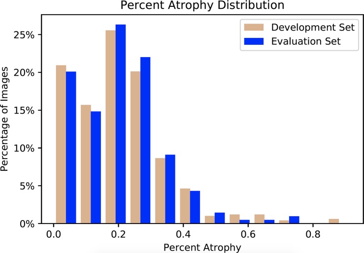
All meibography images were randomly allocated into the following two sub-datasets: development and evaluation. The former was used for developing the deep learning algorithm, while the latter was for evaluating the performance of the algorithm. The percent atrophy distributions of the two datasets were very similar as shown in Figure 2. This minimized the scenario differences between training and evaluation. For algorithm development, the development dataset was further divided randomly into 2 subsets, a train and validation set. The images in the train set were used to train the deep learning model, while the validation set was used for tuning the model hyperparameters (e.g., network architectures, learning rate, etc.). The evaluation dataset, which did not have any overlapping image with the development dataset, was evaluated using the model that achieved the best performance from the validation set. The patient demographics and atrophy severity of the development and evaluation datasets can be found in Table 2 and Figure 3.

Figure 2.

Percent atrophy distribution of the development and evaluation datasets. The distributions of the two sets are similar, indicating the scenario differences between training and evaluation are minimized.

Figure 3.

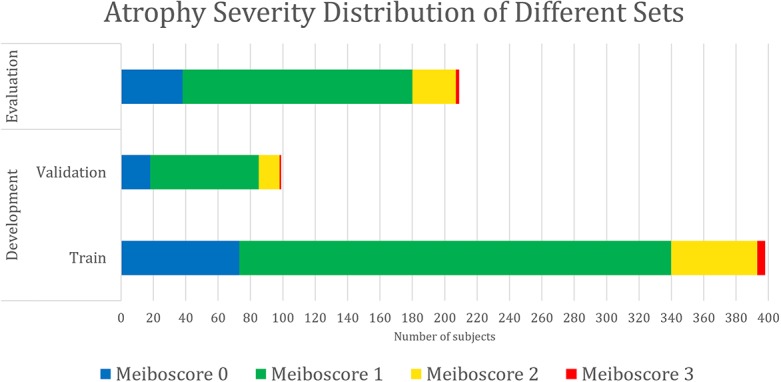
Data composition by atrophy severity. The meiboscore distributions of the train, validation, and evaluation sets are similar, indicating the scenario differences among training, validation, and evaluation are minimized.

Algorithm Design and Training

In computer vision, image segmentation is the process of partitioning an image into multiple segments.23,24 Earlier methods first extracted hand-engineered features of the image, and then used the features to classify pixels independently.25–27 More recently, deep learning methods incorporated feature extraction and classification together into a unified framework, and achieved the state-of-the-art in image segmentation.11,28 A deep learning algorithm was built upon the pyramid scene parsing network29 to segment the atrophy and eyelid region of a given meibography image, and then the percent atrophy was calculated (Fig. 4).

Figure 4.

The pipeline to evaluating meibography atrophy. The network aims to predict the atrophy area (white part in the right image) and the total eyelid area (white and gray part in the right image). Based on the predicted mask, the percent atrophy can be calculated.

The input to the neural network was a meibography image. The network could be considered as several stages of computations, parameterized by millions of parameters, and mapped the input image to the output segmentation masks of MG atrophy and eyelid area. Additionally, the network generated a vector indicating if MG atrophy existed in a given meibography image. The auxiliary output helped improve the segmentation performance by providing additional information. The final optimization goal was to have both correct segmentation and atrophy existence vector prediction.

Parameters of a neural network were determined by training the network on the development dataset. The network was repeatedly given images with known ground truth (the segmentation masks of atrophy and eyelid area, as well as atrophy existence vectors in our model). The model predicted the segmentation masks and atrophy existence vector of the given meibography image, and adjusted its parameters over the training process to make predictions increasingly more similar to the ground truth. The parameters of the model were optimized using stochastic gradient descent30 and the model performance was evaluated by the validation set every epoch. When atrophy area and eyelid area were predicted, the percent atrophy can be calculated as follows:

A hyperparameter search was performed on the network architectures, data-augmentation techniques, learning rate, auxiliary loss ratio, and learning-rate decreasing policy. The hyperparameters, which attained the best performance over the validation set, was selected. The convolutional neural networks were developed using the PyTorch31 deep learning framework. The proposed networks were repeatedly trained and evaluated on two NVIDIA GeForce GTX 1080 GPUs with NVIDIA CUDA v8.0 and NVIDIA cuDNN v5.1 acceleration (NVIDIA, Santa Clara, CA).

Evaluation Protocol

Evaluating the performance of the trained deep model was necessary. First, when performing the extensive tuning of hyperparameters on the training set, the model was evaluated on the validation set to select the hyperparameters that achieved the best performance. Additionally, once the best-performance model was obtained, the performance on the evaluation set was further evaluated to obtain the final performance. The algorithmic performance, including segmentation, percent atrophy, and meiboscore grading performance, was also examined.

Atrophy Segmentation

Two evaluation metrics were adopted to comprehensively assess the similarity between the predicted MG atrophy region and the ground-truth atrophy region.

Accuracy (or pixel accuracy)

In atrophy segmentation example, the atrophy region is referred to as our region of interest (ROI). To evaluate the similarity between network predictions and the ground truth, the label of ROI is denoted as class , while the rest as class . In Table 3, is denoted as the number of pixels of class predicted to belong to class , as the number of correctly classified ROI pixels (true positives, TP), as the number of pixels wrongly classified as ROI (false positives, FP), as true negative (TN), and as false negative (FN). If the total pixel of the input image was , + + + . Thus, accuracy (abbreviated as ACC) is defined as follows:

Table 3.

Confusion Matrix for Illustrating Segmentation Evaluation Metric Mean IU

	Class	Ground-Truth
Predicted		True positive # (TP)	False positive # (FP)
		False negative # (TN)	True negative # (FN)

Similarly, in total eyelid area segmentation example, the eyelid region would be the ROI. ACC reports the percentage of pixels in the image that is correctly classified. However, this metric sometimes provides misleading results when ROI is small, as the measure would be biased by mainly reporting how well non-ROI cases are identified.

Mean IU

Mean intersection over union (mean IU, or Jaccard index) quantifies the percent overlap between the target mask and our prediction output. It measures the number of pixels common between the target and prediction masks divided by the total number of pixels present across both masks. Denoting ground truth ROI segmentation mask as ground-truth (GT), network predicted segmentation mask as prediction, mean IU32 could be written as following:

Intuitively, Equation 3 is analogous to harmonic average of the precision and recall, F1-score, which was defined as , and provided a more “comprehensive'' evaluation—the method considered both precision and recall. For segmentation tasks, higher mean IU value indicated higher alignment of the algorithm prediction with the ground-truth.

In summary, ACC reflects the performance of pixel-wise classification accuracy, while mean IU for how the predicted ROI segmentation mask overlaps with the real counterpart. Mean IU is considered as a stricter evaluation metric than ACC in terms of segmentation. Both evaluation metrics for each image in the evaluation dataset and the calculated average score of all images were reported.

Percent Atrophy

Percent atrophy from the atrophy masks (Equation 1) can be calculated, and the percent atrophy performance of algorithm prediction can also be evaluated against the ground-truth. One standard way is to compute the atrophy ratio difference over the evaluation set and compute the root-mean-square deviation (RMSD) as follows:

where is the real atrophy ratio of image defined in Equation 1, represent the atrophy ratio predicted by the neural network. is the total number of images in evaluation set. Intuitively, Equation 4 reflects the mean difference between predicted percent atrophy and ground truth over all the images in the evaluation set. RMSD could also be considered as the error made by the algorithm when predicting the percent atrophy of an image.

Converting to Meiboscores

Percent atrophy, as a numeric indicator, provides substantial information on the MG atrophy severity of a meibography image. In order to compare with human clinicians' performance, the numeric ratios were converted back to the meiboscore.

From the meibography images with different percent atrophy in Figure 1, images near the grading transition limits (0%, 33%, 66%) were very similar and difficult to classify. A tolerance threshold near the grading transition limit was necessary. The converting criteria in Table 1 was applied with a relaxed standard. As illustrated in Figure 5, the tolerance threshold was set at 0.25%, so classifying images with percent atrophy 0% to 0.25%, 32.75% to 33.25%, and 65.75% to 66.25% either to its ground-truth or adjacent meiboscores were both considered as correct prediction. The same relaxed converting criteria for both human clinicians and algorithm in the experiments were followed for fair comparison.

Figure 5.

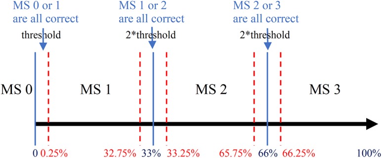
Relaxed meiboscore conversion rule with the tolerance threshold. The percent atrophy to the meiboscore conversion criteria is relaxed with tolerance threshold near the grading transition limits (0%, 33%, 66%). The threshold is set to be 0.25%. Therefore, when percent atrophy falls in 0% to 0.25%, 32.75% to 33.25%, or 65.75% to 66.25%, the correct prediction can be either the ground-truth meiboscore or the adjacent meiboscore.

Results

Network Training Details

Each meibography image and its corresponding segmentation mask(s) were resized to the size of pixels. During training, pixels were randomly cropped out of a given meibography image and corresponding annotations in every training epoch for data augmentation. A center crop of pixels was made to a given meibography image and corresponding annotations during the evaluation process for both validation and evaluation datasets.

Different network architectures (SqueezeNet, resnet18, resnet34, resnet50), auxiliary loss ratio (for 0–1.0 with grid of 0.1), learning rate, and learning-rate decreasing policy were carefully assessed to obtain the best performance of the network on the validation dataset (the best performance of the network over the validation set was resnet50, auxiliary loss ratio 0.1, learning rate 1e-3, 200 epochs in total, with learning rate decrease at 100, 150, and 180, respectively). The algorithm performance of the model on the evaluation dataset is reported.

Algorithm Performance

The baseline characteristics of the training and evaluation dataset were described in Table 2. Development and evaluation dataset had similar characteristics regarding patient demographics and MG atrophy severity.

Table 4 shows the ACC, mean IU, and RMSD of meibography images with different meiboscores. Note that images with meiboscore of grade 0 do not have atrophy so there are no corresponding ACC and mean IU. The performance of meiboscore of grade 0 can however be measured by RMSD and meiboscore grading accuracy. Regarding atrophy segmentation, ACC was higher than mean IU. The instance average ACC values were 97.6% and 95.5% for eyelid and atrophy, respectively, while mean IU values were 95.4% and 66.7% for eyelid and atrophy, respectively. Regarding mean IU for different gland atrophy severity, mean IU was the lowest for meiboscore of grade 3 samples, which only included five images in the training set and only two in evaluation set. Regarding percent atrophy prediction performance, the instance average error was 6.7%. Although images with different meiboscores had relatively similar RMSD, the RMSD value was the highest at 9.0% for meiboscore of grade 1 and the lowest at 5.7% for meiboscore of grade 2. Although the intention was to capture each subject for one single visit, there were three subjects (providing a total of 10 images) from 467 subjects (0.6% subjects) returned to the research facility for two visits within at least a 2-year time lapse. Therefore, a 10-fold cross validation was performed to confirm that the images obtained from the repeated visits would not bias the study results. The results (e.g., mean and standard deviation of ACC, mean IU, and RMSD) were reported in Table 5. Specifically, the development and evaluation sets were randomly split 10 times according to the number of images of each meiboscore category presented in Table 2. The algorithm was trained on different development sets and evaluated on the corresponding evaluation sets for 10 times. Figure 6 plots the predicted percent atrophy versus ground-truth percent atrophy. While most of the points fall on the ideal line (percent atrophy prediction equals to ground-truth), the deep learning algorithm tends to give higher percent atrophy for some cases of meiboscore of grade 0. This is because the algorithm has been trained to be sensitive to even small atrophy, which might have been ignored by clinicians. The errors are greatly reduced when converting to meiboscores using the relaxed criteria as described in the “evaluation protocols” section.

Table 4.

Performance of the Algorithm (%)

	Percent Eyelid Area		Percent Atrophy Area		Percent Atrophy, RMSD
	ACC	Mean IU	ACC	Mean IU
Meiboscore 0	97.9	96.1	/	/	9.0
Meiboscore 1	97.5	95.5	95.7	64.6	6.2
Meiboscore 2	97.6	95.6	94.5	78.3	5.7
Meiboscore 3	91.9	82.1	86.8	63.7	6.9
Class average accuracy	96.3	92.3	92.4	68.8	7.0
Instance average accuracy	97.6	95.5	95.4	66.7	6.7

Table 5.

Performance of the Algorithm Under 10-Fold Cross Validation (%)

	Percent Eyelid Area		Percent Atrophy Area		Percent Atrophy, RMSD
	ACC	Mean IU	ACC	Mean IU
Meiboscore 0	98.0 ± 0.4	96.0 ± 0.5	/	/	9.8 ± 0.8
Meiboscore 1	97.6 ± 0.3	95.4 ± 0.6	96.1 ± 1.7	65.9 ± 1.8	5.6 ± 0.6
Meiboscore 2	97.9 ± 0.5	96.0 ± 0.9	94.6 ± 1.9	77.3 ± 1.8	7.4 ± 1.6
Meiboscore 3	92.4 ± 2.0	83.8 ± 4.0	85.1 ± 3.9	61.6 ± 4.5	7.3 ± 2.0
Class average accuracy	96.4 ± 0.8	92.8 ± 1.5	91.9 ± 2.5	68.3 ± 2.7	7.5 ± 1.3
Instance average accuracy	97.6 ± 0.4	95.5 ± 0.7	95.7 ± 1.8	67.6 ± 1.8	6.6 ± 0.8

Figure 6.

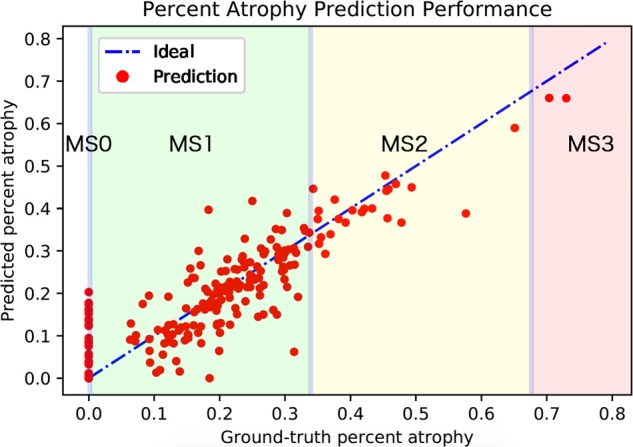
Algorithm-predicted percent atrophy versus ground-truth percent atrophy. The average RMSD of the predicted percent atrophy is 6.7%. While most of the points fall on the ideal line (percent atrophy prediction equals to the ground-truth), more percent atrophy errors occurred for meiboscore of grade 0. Note that the errors are greatly eliminated when applying relaxed meiboscore conversion criteria. The thresholds near grading transition limits are marked in blue.

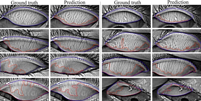
Figure 7 visualizes the atrophy region and eyelid region segmentation results of clinician team and computer. From the visualization, the human segmentation and computer segmentation appear to be very similar, especially for eyelid region segmentations.

Figure 7.

Eyelid (outlined in blue) and atrophy (outlined in red) segmentations from the deep learning algorithm versus the ground-truth. Rows 1 to 4 refer to meiboscores of grade 0 to 3, respectively. The first and third columns are ground-truth images from the annotators, while the second and fourth columns are algorithm predictions. The algorithm predictions shared high visual similarity with the ground-truth, especially for eyelid region segmentation.

Human Clinician's Performance

The confusion matrix is a specific table layout that allows visualizations of how two identities perform the same classification task. Table 6 shows the confusion matrices of study clinician and single clinician. The highest agreement percentage was 69% for meiboscore of grade 1, while the lowest was 40% for meiboscore of grade 3. The kappa score is 0.324 for clinical team and the LCI, which led to a fair agreement according to Landis et al.33 In other words, clinicians' ratings have high variability.

Table 6.

Confusion Matrix of LCI and Clinical Meiboscore (%)

Note: Warm colors with small values indicate less agreement.

Comparing Meiboscores

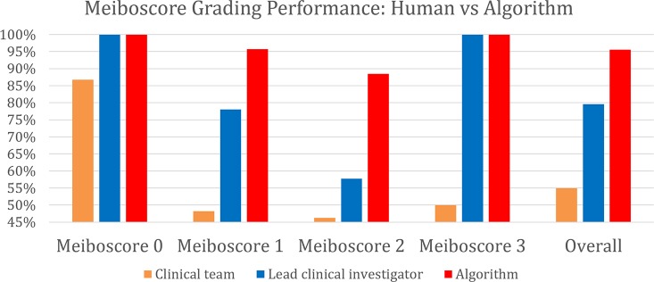
The meiboscore grading performance of the algorithm was compared against the ground-truth meiboscores. The ground-truth meiboscores were obtained from the percent atrophy (calculated from human-annotated segmentation masks) using Table 1. Tables 7 and Figure 8 show the meiboscore grading performance by the algorithm, clinical team (clinical meiboscore), and the LCI meiboscore. The algorithm achieves 95.6% overall grading accuracy, which outperforms the LCI meiboscore by 16.0% and clinical team meiboscore by 40.6%. For each meiboscore, the algorithm also largely outperforms human clinicians. Figure 9 depicts some failure cases in meiboscore grading of human clinicians and our algorithm. Failure cases appear for both human-assigned and algorithm meiboscores when percent atrophy is near the meiboscore grading transition limits.

Table 7.

Meiboscore Grading Performance of Clinicians and Algorithm (%)

	Percent Clinical Team	Percent Lead Clinical Investigator	Percent Algorithm
Meiboscore 0	86.8	100.0	100.0
Meiboscore 1	48.2	78.0	95.7
Meiboscore 2	46.2	57.7	88.5
Meiboscore 3	50.0	100.0	100.0
Class average accuracy	57.8	83.9	96.1
Instance average accuracy	55.0	79.6	95.6

Figure 8.

Meiboscore grading performance of the clinical team, the LCI, and the proposed algorithm. The algorithm outperforms the LCI meiboscore by 16.0% and clinical team meiboscore by 40.6%.

Figure 9.

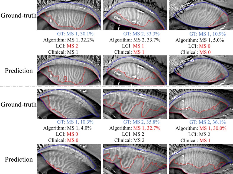
Examples of failure cases in meiboscore (MS) grading: human clinicians versus machine algorithm. GT refers to the ground-truth. Failure cases occur for both clinicians and the algorithm for the images with percent atrophy near the meiboscore grading boundaries.

Discussion

The present work introduces a deep learning approach to automatically predict the MG atrophy region and compute percent atrophy in the meibography image. The proposed method has the following three advantages: (1) low variability and high repeatability (test–retest reliability); (2) output quantitative result rather than qualitative description (e.g., specific gland atrophy region and numeric percent atrophy prediction); and (3) efficient and low cost. The average processing time per meibography image was approximately 0.29 seconds (experiments were performed on one NVIDIA GeForce GTX 1080 GPU). This means that more than 1000 unprocessed or raw meibography images can be evaluated for atrophy severity in 5 minutes without additional human resource needed.

The algorithm also has very high performance. Accuracies of eyelid area and atrophy area achieve 97.6% and 95.4%, respectively, and the overall mean IUs are 95.5% and 66.7%, respectively. Our algorithm achieves a 95.6% overall grading accuracy and outperforms the LCI meiboscore grading accuracy by 16%. From the visualization of the predicted eyelid and atrophy segmentation, the algorithm predictions have high visual similarity with the ground-truth annotations.

In all, the proposed algorithm achieves very high performance with low variability and high repeatability in evaluating MG atrophy from meibography images. Additionally, the proposed algorithm could potentially be applied to other similar image segmentation tasks in the clinical community.

Furthermore, regarding MG atrophy evaluation, numeric percent atrophy reporting is a better assessment than simple meiboscore grading. It is challenging to distinguish different meiboscores when the percent atrophy is near the grading transition limits (0%, 33%, 66%), because no distinct changes observed for meibography images in these regions. Forcing a strict meiboscore near the boundary can lead to grading inconsistency and variability. When applying numeric percent atrophy, however, clinicians would not need to worry about the images with percent atrophy near these grading transition limits. Additionally, there are several different grading scales for gland atrophy.4,5 Conversion between different grading system is impossible as the percentage information already got lost. Numeric percent atrophy adopted in this study overcomes the above-mentioned problems.

In conclusion, a deep learning approach to automatically evaluate the MG atrophy in meibography images has been developed. The system has high accuracy, repeatability, and low variability, as well as outperforming human clinicians by a significant margin. The quantitative outputs (specific atrophy region and percent atrophy) provide valuable information of MG atrophy severity of the meibography image. In the present work, our deep learning system could only predict MG atrophy region, but not individual MG morphology. Future work can explore how deep learning can automatically analyze MG morphologic characteristics (e.g., gland number, width, intensity, and tortuosity), which can be potentially important for advancing the efficiency of MGD treatment and management. Capturing human expert knowledge with data-driven, deep learning systems is the future of image-based medical diagnosis. The possibility of using deep learning methods for clinical diagnosis in ocular surface diseases is shown. New surveys can be enabled by automatic and quantitative evaluations, opening up many exciting opportunities for targeted medical treatment and drug discoveries.

References

- 1.Baudouin C, Messmer EM, Aragona P, et al. Revisiting the vicious circle of dry eye disease: a focus on the pathophysiology of meibomian gland dysfunction. Br J Ophthalmol. 2016;100:300–306. doi: 10.1136/bjophthalmol-2015-307415. [DOI] [PMC free article] [PubMed] [Google Scholar]
- 2.Arita R, Itoh K, Maeda S, et al. Proposed diagnostic criteria for obstructive meibomian gland dysfunction. Ophthalmology. 2009;116:2058–2063. doi: 10.1016/j.ophtha.2009.04.037. [DOI] [PubMed] [Google Scholar]
- 3.Giannaccare G, Vigo L, Pellegrini M, Sebastiani S, Carones F. Ocular surface workup with automated noninvasive measurements for the diagnosis of meibomian gland dysfunction. Cornea. 2018;37:740–745. doi: 10.1097/ICO.0000000000001500. [DOI] [PubMed] [Google Scholar]
- 4.Arita R, Itoh K, Inoue K, Amano S. Noncontact infrared meibography to document age-related changes of the meibomian glands in a normal population. Ophthalmology. 2008;115:911–915. doi: 10.1016/j.ophtha.2007.06.031. [DOI] [PubMed] [Google Scholar]
- 5.Pult H, Nichols JJ. A review of meibography. Optom Vis Sci. 2012;89:E760–E769. doi: 10.1097/OPX.0b013e3182512ac1. [DOI] [PubMed] [Google Scholar]
- 6.Pflugfelder SC, Tseng SCG, Sanabria O, et al. Evaluation of subjective assessments and objective diagnostic tests for diagnosing tear-film disorders known to cause ocular irritation. Cornea. 1998;17:38–56. doi: 10.1097/00003226-199801000-00007. [DOI] [PubMed] [Google Scholar]
- 7.Nichols JJ, Berntsen DA, Mitchell GL, Nichols KK. An assessment of grading scales for meibography images. Cornea. 2005;24:382–388. doi: 10.1097/01.ico.0000148291.38076.59. [DOI] [PubMed] [Google Scholar]
- 8.Pult H, Riede-Pult B. Comparison of subjective grading and objective assessment in meibography. Contact Lens Anterior Eye. 2013;36:22–27. doi: 10.1016/j.clae.2012.10.074. [DOI] [PubMed] [Google Scholar]
- 9.Krizhevsky A, Sutskever I, Hinton GE. ImageNet classification with deep convolutional neural networks. 2012. pp. 1097–1105. Available at: http://papers.nips.cc/paper/4824-imagenet-classification-with-deep-convolutional-neural-networks. Accessed February 8, 2019.
- 10.Ronneberger O, Fischer P, Brox T. International Conference on Medical Image Computing and Computer-Assisted Intervention. Switzerland AG: Springer; 2015. U-Net: convolutional networks for biomedical image segmentation; pp. 234–241. [Google Scholar]
- 11.Chen L-C, Papandreou G, Kokkinos I, Murphy K, Yuille AL. DeepLab: semantic image segmentation with deep convolutional nets, atrous convolution, and fully connected CRFs. IEEE Trans Pattern Anal Mach Intell. 2018;40:834–848. doi: 10.1109/TPAMI.2017.2699184. [DOI] [PubMed] [Google Scholar]
- 12.Ting DSW, Cheung CY-L, Lim G, et al. Development and validation of a deep learning system for diabetic retinopathy and related eye diseases using retinal images from multiethnic populations with diabetes. JAMA. 2017;318:2211. doi: 10.1001/jama.2017.18152. [DOI] [PMC free article] [PubMed] [Google Scholar]
- 13.Nayak J, Bhat PS, Acharya R, Lim CM, Kagathi M. Automated identification of diabetic retinopathy stages using digital fundus images. J Med Syst. 2008;32:107–115. doi: 10.1007/s10916-007-9113-9. [DOI] [PubMed] [Google Scholar]
- 14.Decencière E, Zhang X, Cazuguel G, et al. Feedback on a publicly distributed image database: the Messidor database. Image Anal Stereol. 2014;33:231. [Google Scholar]
- 15.Liu Y, Gadepalli K, Norouzi M, et al. Detecting cancer metastases on gigapixel pathology images. Mar, 2017. Available at: http://arxiv.org/abs/1703.02442. Accessed February 8, 2019.
- 16.Ehteshami Bejnordi B, Veta M, Johannes van Diest P, et al. Diagnostic assessment of deep learning algorithms for detection of lymph node metastases in women with breast cancer. JAMA. 2017;318:2199. doi: 10.1001/jama.2017.14585. [DOI] [PMC free article] [PubMed] [Google Scholar]
- 17.Esteva A, Kuprel B, Novoa RA, et al. Dermatologist-level classification of skin cancer with deep neural networks. Nature. 2017;542:115–118. doi: 10.1038/nature21056. [DOI] [PMC free article] [PubMed] [Google Scholar]
- 18.Litjens G, Kooi T, Bejnordi BE, et al. A survey on deep learning in medical image analysis. Med Image Anal. 2017;42:60–88. doi: 10.1016/j.media.2017.07.005. [DOI] [PubMed] [Google Scholar]
- 19.Ching T, Himmelstein DS, Beaulieu-Jones BK, et al. Opportunities and obstacles for deep learning in biology and medicine. J R Soc Interface. 2018;15:20170387. doi: 10.1098/rsif.2017.0387. [DOI] [PMC free article] [PubMed] [Google Scholar]
- 20.Markoulli M, Duong TB, Lin M, Papas E. Imaging the tear film: a comparison between the subjective Keeler Tearscope-PlusTM and the Objective Oculus® Keratograph 5M and LipiView® Interferometer. Curr Eye Res. 2018;43:155–162. doi: 10.1080/02713683.2017.1393092. [DOI] [PubMed] [Google Scholar]
- 21.Yeh TN, Lin MC. Repeatability of meibomian gland contrast, a potential indicator of meibomian gland function. Cornea. 2019 Nov;38:256–261. doi: 10.1097/ICO.0000000000001818. [DOI] [PMC free article] [PubMed] [Google Scholar]
- 22.Schindelin J, Arganda-Carreras I, Frise E, et al. Fiji: an open-source platform for biological-image analysis. Nat Methods. 2012;9:676–682. doi: 10.1038/nmeth.2019. [DOI] [PMC free article] [PubMed] [Google Scholar]
- 23.Pal NR, Pal SK. A review on image segmentation techniques. Pattern Recognit. 1993;26:1277–1294. [Google Scholar]
- 24.Malik J, Arbeláez P, Carreira J, et al. The three R's of computer vision: recognition, reconstruction and reorganization. Pattern Recognit Lett. 2016;72:4–14. [Google Scholar]
- 25.Shotton J, Johnson M, Cipolla R. Semantic texton forests for image categorization and segmentation. 2008 IEEE Conference on Computer Vision and Pattern Recognition. Paper presented at. Ankorage, AK, June 23–28, 2008.
- 26.Ladický Ľ, Sturgess P, Alahari K, Russell C, Torr PHS. Author, author, eds. European Conference on Computer Vision. Berlin: Springer; 2010. What, where and how many? Combining object detectors and CRFs; pp. 424–437. [Google Scholar]
- 27.Sturgess P, Alahari K, Ladicky L, Torr PHS. Combining appearance and structure from motion features for road scene understanding. Procedings of the British Machine Vision Conference 2009. Paper presented at. London, UK, September 7–10, 2009.
- 28.Badrinarayanan V, Kendall A, Cipolla R. SegNet: a deep convolutional encoder-decoder architecture for image segmentation. IEEE Trans Pattern Anal Mach Intell. 2017;39:2481–2495. doi: 10.1109/TPAMI.2016.2644615. [DOI] [PubMed] [Google Scholar]
- 29.Zhao H, Shi J, Qi X, Wang X, Jia J. Pyramid scene parsing network. Available at: https://github.com/hszhao/PSPNet. Accessed February 8. 2019.
- 30.Bottou L. Lechevallier Y, Saporta G, editors. Large-scale machine learning with stochastic gradient descent. Proceedings of COMPSTAT'2010. Heidelberg: Physica-Verlag HD. 2010. pp. 177–186. In. eds.
- 31.Paszke A, Gross S, Chintala S, et al. Automatic differentiation in PyTorch. Available at: https://pdfs.semanticscholar.org/b36a/5bb1707bb9c70025294b3a310138aae8327a.pdf. Accessed February 8. 2019.
- 32.Long J, Shelhamer E, Darrell T. Fully convolutional networks for semantic segmentation. Available at: https://www.cv-foundation.org/openaccess/content_cvpr_2015/app/2B_011.pdf. Accessed March 28. 2018. [DOI] [PubMed]
- 33.Landis JR, Koch GG. The measurement of observer agreement for categorical data. Biometrics. 1977;33:159. [PubMed] [Google Scholar]