Detecting mammographically occult cancer in women with dense breasts using deep convolutional neural network and Radon Cumulative Distribution Transform

Abstract.

We have applied the Radon Cumulative Distribution Transform (RCDT) as an image transformation to highlight the subtle difference between left and right mammograms to detect mammographically occult (MO) cancer in women with dense breasts and negative screening mammograms. We developed deep convolutional neural networks (CNNs) as classifiers for estimating the probability of having MO cancer. We acquired screening mammograms of 333 women (97 unilateral MO cancer) with dense breasts and at least two consecutive mammograms and used the immediate prior mammograms, which radiologists interpreted as negative. We used fivefold cross validation to divide our dataset into a training and independent test sets with ratios of 0.8:0.2. We set aside 10% of the training set as a validation set. We applied RCDT on the left and right mammograms of each view. We applied inverse Radon transform to represent the resulting RCDT images in the image domain. We then fine-tuned a VGG16 network pretrained on ImageNet using the resulting images per each view. The CNNs achieved mean areas under the receiver operating characteristic (AUC) curve of 0.73 (standard error, SE = 0.024) and 0.73 (SE = 0.04) for the craniocaudal and mediolateral oblique views, respectively. We combined the scores from two CNNs by training a logistic regression classifier and it achieved a mean AUC of 0.81 (SE = 0.032). In conclusion, we showed that inverse Radon-transformed RCDT images contain information useful for detecting MO cancers and that deep CNNs could learn such information.

1. Introduction

The purpose of this study was to develop a classifier that provides women who have dense breasts and a negative screening mammogram the likelihood of having a nonmammographically visible breast cancer. This information would help women with dense breasts and their physicians decide if additional imaging, with ultrasound or magnetic resonance imaging (MRI), is necessary.

Mammographically occult (MO) cancer is a breast cancer that is visually subtle, or occluded by other breast tissue, such that radiologists missed the cancer. The incidence rate of MO cancer is higher in women with dense breasts, as dense-breast tissue can hide cancer.^1,2 As a result, screening sensitivity via mammography is lower for women with dense breasts. In this respect, physicians may recommend that women with dense breasts undergo additional screening with MRI or ultrasound, which are more sensitive tests than mammography. However, these additional screening modalities are not perfect, as they have higher false-positive rates and cost more than mammography (especially, MRI).^3–5 Unlike a false-positive screening mammogram, which would lead to more imaging, a false-positive MRI or ultrasound can lead directly to a breast biopsy. Hence, it would be beneficial to provide information about the likelihood of having an MO breast cancer for women with dense breasts, because this would allow those women to make a more informed decision about whether or not to have additional screening.

In our previous study, we introduced the Radon Cumulative Distribution Transform (RCDT)⁶ as an image transformation to highlight the subtle differences between left and right mammograms and showed that we can use features extracted from the transformed images to detect MO cancers from negative screening mammograms.⁷ Specifically, we found that a linear combination of evenly distributed plaid or check patterns can characterize the left–right normal breast tissue difference, whereas MO cancer cases exhibit more complex patterns than plaid or check patterns. We showed that, to distinguish the MO cancer cases from the normal controls, we can use the plaid or check patterns. However, it is difficult to explain what shape and texture in the RCDT image correspond to the MO cancer.

Deep convolutional neural network (CNN) is currently the-state-of-art method for image classification, detection, and interpretation, especially in the tasks of natural scene interpretation.⁸ The medical imaging community has actively adopted deep CNN for various imaging tasks, including detection, diagnosis, and prognosis of various diseases and body parts (e.g., breast),^9–11 and showed promising performances or even outperformed the human experts for some diseases (e.g., diabetic retinal detection¹²).

To properly train deep CNNs, one requires many human labeled images. Most CNNs use ImageNet as the training dataset. ImageNet⁸ is a collection of natural scene images in 1000 categories with at least 1000 per category, which sums up to 1.4 million images in total. However, establishing such a number of labeled medical images is time-consuming and expensive. Thus, researchers in the medical imaging field have been utilizing transfer learning instead. Transfer learning is the act of reusing the knowledge learned via solving a problem on a related but different problem. In deep learning, transfer learning is reusing or fine-tuning a pretrained network on a large dataset, typically ImageNet, to solve new tasks. By using transfer learning, one only needs a few hundred or a thousand images to fine-tune the CNN for new images and new tasks.

Lower layers of a CNN detect low-level image features, such as the edge, and upper layers extract more abstract information, as the layers tend toward the output of the network. However, it is not useful to know where and what patterns/features CNNs are focusing on. Researchers proposed a class activation map (CAM)^13,14 as a solution, when a CNN analyzes an image for a given task.

Thus, we developed a CNN-based classifier to analyze the RCDT image of mammograms for distinguishing women with MO cancer from normal controls. Specifically, we fine-tuned (transfer learning) a CNN (pretrained on ImageNet) on RCDT images. Finally, we analyzed how the trained CNN perceived the given images by using the CAM approach.

2. Methods

2.1. Dataset

Under an Institutional Review Board (IRB) approved protocol, we used screening digital mammograms (DMs) of 333 women with dense-breast tissue rated as breast imaging reporting and data system (BI-RADS) breast density level 3 or level 4 (Table 1). Among the 333 women, 236 were normal with two consecutive prior negative screening DMs, and 97 had a unilateral MO cancer, where radiologists interpreted them as normal mammograms until the cancer was visible in the index screening mammogram. In this study, we used the most recent prior screening mammograms, where women with MO cancer and normal controls had negative screening mammograms.

Table 1.

Characteristics of mammogram dataset.

Total number of subjects		MO cancer	Controls
		97	236
Subject age (years)	Mean (min, max)	56.2 (39, 70)	48.5 (36, 70)
BI-RADS breast density	3	91	171
	4	6	67
Diagnosisa at index exam	IDC and DCIS	40 (41%)	N/A
	IDC only	27 (28%)
	DCIS	22 (23%)
	IMC	4 (4%)
	ID and ILC	2 (2%)
	ILC only	2 (2%)

^aIDC, Invasive ductal carcinoma; IMC, invasive mammary carcinoma (a tumor that has mixed characteristics of both ductal and lobular carcinoma); ILC, invasive lobular carcinoma; DCIS: ductal carcinoma in situ.

2.2. Radon Cumulative Distribution Transform

RCDT is a nonlinear and invertible image transform that can represent a given image $I$ in terms of a given template image $I_0$. Let two-dimensional Radon transform on the image $I$ and the template $I_0$ be $\hat{I}=R(I)$ and ${\hat{I}}_0=R(I_0)$, respectively. Then, the RCDT for image $I$ is given as

$$\overline{I}(·,\theta )=(f(·,\theta )-\mathrm{id})\sqrt{{\hat{I}}_0(·,\theta )},$$ (1)

and its inverse transform given as

$$I=R^{-1}\{det[J(g)]({\hat{I}}_0\circ g)\},\text{where}g(t,\theta )=\left[\begin{array}{c}{f}^{-1}(t,\theta )\\ \theta \end{array}\right],$$ (2)

where $J(.)$ is the Jacobian and id refers to the identity function, i.e., $r(x)=x$, $t$ and $\theta$ refers to the displacement and angle in the sinogram. In addition, $f(.,\theta )$ warps $\hat{I}(·,\theta )$ to ${\hat{I}}_0(·,\theta )$, where it satisfies

$${\int }_{-\infty }^{f(t,\theta )}\hat{I}(u,\theta )\mathrm{d}u={\int }_{-\infty }^t{\hat{I}}_0(u,\theta )\mathrm{d}u,\text{for all}\theta \in [0,\pi ].$$ (3)

By using RCDT, we can represent how the intensities of image $I$ and their locations differ from $I_0$ in terms of each angle $\theta$ and displacement $t$ from the origin in image space. We set the angle $\theta$ ranged for [0, 180] deg with an increment of 1 deg and set the displacement $t$ ranged for $\{0,\mathrm{sqrt}[\text{length}{(\text{row of image})}^2+\text{length}{(\text{column of image})}^2]\}$ with an increment of 1.

Original RCDT by Kolouri et al.⁶ sets a common image, such as an averaged image of the samples, as a template $I_0$. In our case, using a single common image as a template is not appropriate. This is because radiologists use the lateral difference, i.e., left and right breast tissue differences, as a method to detect abnormalities in a screening exam. Thus, we set the left breast image as template $I_0$ and the contralateral mammogram as target $I$ for normal controls. For MO cancer cases, we set the non-MO cancer side as template $I_0$ and the MO cancer side as target $I$ for MO cancer cases. Then, we applied RCDT on $I$ to $I_0$ using the above equations to amplify subtle suspicious signals existing in mammograms.

Kolouri et al.⁶ showed that translation and scaling of pixels in images, which are nonlinear operations in image space, are linear in RCDT space. In addition, it was also shown that complex patterns in image space can be represented as linear combinations of simple patterns in RCDT space. As left and right breast tissues are similar in most cases, a suspicious signal can be visible by comparing the breast tissues laterally, a technique used by radiologists. However, we assumed that MO cancer may not be visible at all to the naked eye—it is just very subtle or too complex to distinguish from normal breast tissue. As RCDT can decompose complex patterns in image space into linear combinations of simple patterns in RCDT space, we assumed that RCDT could decompose the subtle cancerous signal from the normal breast tissue by using RCDT to analyze the difference in left and right breast tissues. Figure 1 shows the potential of RCDT to identify MO cancer by decomposing or highlighting the subtle difference between left and right breast tissues [Figs. 1(a) and 1(b), circled in red], which direct difference image [Fig. 1(e)] failed to highlight.

Fig. 1.

An example of the RCDT technique on an example left and right craniocaudal (CC) view images. Using (a) template and (b) target, we can compute (c) RCDT of $I$ in terms of I0. If we apply (d) inverse Radon transformation, we can transform the RCDT image back to image space. The resulting RCDT image in image space highlights the lateral difference, which the (e) direct difference image failed to highlight.

2.3. Preprocessing and Applying Radon Cumulative Distribution Transform on Mammograms

The proposed RCDT is to highlight the left and right breast tissue differences. Thus, breast size difference within the same woman, as well as breast size differences across different women, can impact the output of the RCDT of a mammogram. To minimize this difference, we segmented the breast area using an algorithm that we have developed previously¹⁵ and cropped the segmented breast area using a tight rectangular box. The algorithm removed any soft tissue other than the breast. For the mediolateral oblique view, the algorithm removes the pectoral muscle (middle, second row in Fig. 2). Then, we resized each segmented image to $800\times 500\text{pixels}$ using bicubic interpolation. After that, we matched the orientation of the right and left mammograms by horizontally flipping the right side mammograms. After the above procedures, breasts depicted in the mammogram images were similar in size and orientation.

Fig. 2.

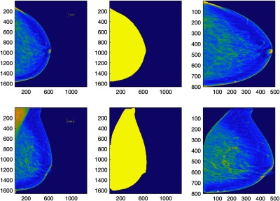
The first column shows the left CC and MLO view mammograms in the original size. The second column shows the breast area mask created by the automated algorithm.¹⁵ We then segmented the breast area by applying the breast area mask on the original mammograms and then cropping the breast area using tight rectangular window. After that, we resized the resulting segmented image to $800\times 500\text{pixels}$ as shown in the third column of the figure.

The network weights of the pretrained CNN were based on natural scenes such as cats and dogs, and therefore fine-tuning the pretrained CNN directly on RCDT images may not work, as their image domains are different. Thus, we transformed the RCDT images back to the image domain by applying the inverse Radon transformation. In addition, we applied contrast-limited adaptive histogram equalization¹⁶ to the resulting images to enhance patterns in the images that are candidates for developing classifiers. Figures 3(d), 3(e), 3(i), and 3(j) show the inverse Radon-transformed RCDT image of the left and right CC view mammograms and its contrast-enhanced version of normal woman and woman with MO cancer, respectively.

Fig. 3.

(a) A template (left breast) and (b) a target (right breast) of the CC view mammogram, its (c) RCDT image, (d) the inverse Radon transform of the RCDT image, and (e) its contrast-enhanced version of a normal woman. (f) A template (normal side, left breast) and (g) a target (MO cancer side, right breast) of the CC view mammogram, (h) its RCDT image, (i) the inverse Radon transform of the RCDT image, and (j) its contrast-enhanced version of a woman with MO cancer. The arrows indicate the location of MO cancer that can be found in the subsequent year’s mammogram.

2.4. Convolutional Neural Network Architecture

Training a deep CNN from scratch is difficult, because it is time-consuming and expensive to collect thousands of curated medical images. Thus, researchers use transfer learning instead, in which a pretrained network is used for a similar but different imaging task. One can fine-tune the pretrained networks with a much smaller dataset, a few hundred cases, to solve their own target-imaging task.

This study used the VGG16¹⁷ network pretrained on ImageNet as a basis network. We fine-tuned the network using our dataset to estimate the probability of having MO cancer in negative screening mammograms. We removed the classification, softmax, and the last fully connected layer (fc8) from the pretrained VGG16 network, to modify the network for our study, which is a two-class problem (normal versus MO cancer). We adopted a “soft-landing” approach to reduce the number of neurons in fully connected layers gradually from 4096 neurons of the “fc7” layer of the VGG16 network to the final two-class output (normal and MO cancer). Specifically, we appended two fully connected layers with 100 and 2 neurons followed by softmax and classification layers to the VGG16 network. Note that we appended a batch normalization layer after the fully connected layers with 100 neurons. The batch normalization layer is known for adding better stability and performance on the network.¹⁸ Figure 4 shows the updated VGG16 network used for this study.

Fig. 4.

The VGG16 network structure used for this study. We removed the last fully connected layer (fc8) and appended two fully connected layers, one with an output size of 100 and another with 2, to reduce the number of neurons from the 4096 neurons of the fc7 layer to the final two-class output.

2.5. Training Setup

The input image size of the VGG16 network is $224\times 224\text{pixels}$. We reduced the size of our images with $800\times 500\text{pixels}$ to $400\times 250\text{pixels}$ to make the size of our images compatible to the input size of the VGG16 network.

We used fivefold cross-validation to fully utilize the dataset for training and testing, as well as to reduce the possible bias introduced during training and testing set selection. Each cross-validation fold includes mutually exclusive training and testing sets with an 8:2 ratio. Among the training set samples, we further set aside 10% of the training set to validate the fine-tuned VGG16 network during the training process. We also implemented a data augmentation, including a horizontal and vertical random flip and random cropping, with the $224\times 224$ window. We ran data augmentation as explained above three times for the normal controls. Then, we repeated the data augmentation for MO cancer cases until the number of augmented datasets was similar to that of the augmented normal controls. After the augmentation, the total number of MO cancer cases and normal controls in each cross-validation fold were $702$ and 564, respectively.

We used the NVIDIA Titan X graphic card to fine-tune the above network. We set the learning rate of the newly added layers 10 times higher than the original layers to expedite the learning process for those new layers. We used the Adam optimizer¹⁹ to optimize the network. The training options included (mini-batch size: 16, learning rate: 0.00001, learning rate drop factor: 0.8, learning rate drop period: 5, momentum: 0.9, weight decay: 0.0001). We fine-tuned two VGG16 networks, one for the CC view and another for the MLO view.

2.6. Combining Scores from Convolutional Neural Networks for CC and MLO Views

For each cross-validation fold, we computed the scores (probability of having MO cancer) from two CNNs, one for the CC view and another for the MLO view on the training and test sets. Using the scores from the training set, we trained an ensemble classifier by training a linear regression classifier. A previous study showed that building an ensemble classifier by combining scores from multiple CNNs can reduce the variances of prediction and generalization errors and therefore achieve improved classification performance.²⁰ We used the entire preprocessed images (i.e., contrast-enhanced version of inverse Radon transform of RCDT-processed images) to the input size of the VGG16 network, which is $224\times 224\text{pixels}$. Figure 5 shows how we built an ensemble classifier for detecting MO cancer. In addition to a logistic regression classifier, we tested different types of classifiers, including linear discriminant analysis (LDA) and support vector machine (SVM), to combine scores from two CNNs.

Fig. 5.

An example of how we built an ensemble classifier for detecting MO cancer. The white arrows indicate the location of MO cancer in the mammogram and RCDT images. Note that the mammograms shown in this figure were BI-RADS assessment category 1 (no sign of malignancy). We retrospectively located the MO cancer using the cancer location at the index year (the year that cancer was diagnosed). After the completion of training two CNNs on the training set, we computed the scores or probability of having MO cancer for the held-out test set under fivefold cross validation. We then trained the final ensemble logistic regression classifier to combine the scores from two CNNs. We used the scores of CNNs for the training set to train the final ensemble classifier and used the resulting classifier to combine two scores from CNNs for the test set to the final score for having MO cancer.

2.7. Class Activation Map for Visualizing Where the Convolutional Neural Network Focuses

We analyzed where the trained CNNs look to classify the women with MO cancer from normal controls. The CAM^13,14 can visualize what the trained CNNs are looking at on a given image for a given class. We used the gradient-based method by Selvaraju et al.,¹⁴ as it can be applied to any CNN architectures (unlike CAM by Zhou et al.,¹³ which needs global averaging pooling) to localize where and at what the CNNs are looking on the inverse Radon transformation of RCDT images of MO cancers.

2.8. Training Convolutional Neural Networks from Scratch and without Radon Cumulative Distribution Transform Processing

To show the effectiveness of transfer learning or fine-tuning, we trained the VGG16 network for each view from scratch. In addition, we fine-tuned additional VGG16 networks for each view without the RCDT process. For MO cancer cases, we used the breast mammogram with MO cancer [e.g., Fig. 3(g)] for training, and we used the right breast mammogram [e.g., Fig. 3(b)] for normal controls. We used these networks on a single-side mammogram to show the effectiveness of the RCDT technique for classifying MO cancer cases. We used the same procedure, as explained in Secs. 2.5 and 2.6, to train additional VGG16 networks and combined the scores from the networks on CC and MLO views for classifying MO cancer cases from the normal controls.

3. Results

The fine-tuned VGG16 networks (MLO and CC views) achieved accuracies (number of correct estimates/total number of cases) of 99% to 100% on the training set and 80% on the validation set after 15 epochs. For each cross-validation fold, we conducted receiver operating characteristic (ROC) curve analysis and computed the area under the ROC curve (AUC) for the fine-tuned networks. The VGG16 network trained for analyzing the CC view achieved an average AUC of 0.73 with a standard error (SE) of 0.024 [(min, max) of AUC = (0.67, 0.8)] and another CNN trained for analyzing the MLO view achieved an average AUC of 0.73 with an SE of 0.04 [(min, max) of AUC = (0.66, 0.8)] for classifying MO cancer cases and normal controls on the test dataset for each cross-validation fold.

The final ensemble classifier (logistic regression) was built on the scores from two CNNs. The performance of the ensemble classifier was an average AUC of 0.81 with an SE of 0.032 [(min, max) of AUC = (0.72, 0.88)] for the testing set for each cross-validation fold. LDA and SVM classifiers for combining the scores from CNN achieved similar performances on the test results under a fivefold cross-validation (average AUC of LDA classifiers = 0.81; average AUC of SVM classifiers = 0.8). Figure 6 shows the ROC curves of the final ensemble classifiers for the fivefold cross-validation test set.

Fig. 6.

The ROC curves and their AUC values for the final ensemble classifier under the fivefold cross validation. The AUC values for the final classifier ranged from 0.71 to 0.88.

The VGG16 networks trained from scratch achieved poor accuracies (number of correct estimates/total number of cases) of around 50% to 60% on both the training and the validation sets throughout the training process. This shows the effectiveness of transfer learning, or fine-tuning, for the dataset with a limited number of samples.

The VGG16 networks trained directly on mammograms without RCDT achieved an average AUC of 0.67 with an SE of 0.029 for the CC view [(min, max) of AUC = (0.57, 0.73)] and 0.69 with an SE of 0.024 for the MLO view [(min, max) of AUC = (0.64, 0.78)]. The final ensemble classifier (logistic regression) was built on the scores from two CNNs. The performance of the ensemble classifier was an average AUC of 0.7 with an SE of 0.022 [(min, max) of AUC = (0.61, 0.74)] for the testing set for each cross-validation fold.

We found that the AUC value of the VGG16 network with the RCDT process is consistently higher than that of the VGG16 network without the RCDT process for each held out test set under the fivefold cross validation. VGG16 with RCDT versus VGG16 without RCDT for each cross-validation test set was given as follows: 0.88 versus 0.72 for first fold, 0.71 versus 0.61 for second fold, 0.87 versus 0.71 for third fold, 0.82 versus 0.71 for fourth fold, and 0.76 versus 0.74 for fifth fold. The difference in averaged AUCs for the VGG16 networks with and without the RCDT process was statistically significant (via paired $t$-test, $p\text{-}\text{value}=0.0115$). This result shows that mammograms with MO cancer has useful information for classifying MO cancer cases, but it was not as effective for RCDT-processed mammograms. As we used RCDT to highlight the lateral breast tissue difference between left and right breast mammograms, RCDT may amplify MO cancer characteristics in mammograms further by comparing the left and right breast tissues in mammograms.

We then analyzed the focal area of the trained CNN using the gradient-weighted class activation map (Grad-CAM) technique. Among the five trained CNNs for each fold, we used the one with an AUC value closest to the mean (i.e., CNN trained for fourth fold, with a test AUC of 0.82) for this analysis. Figure 7 shows the Grad-CAM of the MO cancer cases for the CC and MLO views of the inverse Radon transformation of RCDT images from the training set (upper row) and another from the test set (bottom row). The figure shows that the trained (fine-tuned) CNNs for both the MLO and CC views look at the area where the pixel intensity changes rapidly, from high intensity to low intensity, or vice versa [Fig. 7(b), where the low intensity thin lines are located, and Figs. 6(d) and 6(h), where pixel intensity drops near the big lump in the middle]. Although there were false-positive locations, the trained CNNs picked up the area where the MO cancer was located (arrows in Fig. 7). This analysis shows that the RCDT can amplify the difference between left and right breast tissues, and certain signatures (sudden dip or hike in intensity in inverse Radon transformation of RCDT images) indicate the MO cancer, where the fine-tuned CNNs were able to learn.

Fig. 7.

The CAM of the fine-tuned CNN for an MO cancer case. Images showing the MO cancer case from (a)–(d) the training set and (e)–(h) the testing set, respectively, which show how it trained to locate the key area for classifying MO cancer cases. Arrows indicate the MO cancer location. MO cancer location was based on the most recent mammogram where the radiologists identified the abnormality. Note that all images shown in this figure are based on the immediate prior mammograms before cancer detection.

4. Discussion

In this study, we developed a classifier to identify women with dense breasts and with MO cancer using the information extracted from RCDT images of their mammograms. We used RCDT to amplify suspicious signals of MO cancer that radiologists could not detect. We utilized deep CNNs to analyze the RCDT images of the mammograms to locate the MO cancer signals. We showed that CNNs could learn and locate the suspicious signals that RCDT amplified.

There is only a small number of previous studies investigating MO cancer. Mainprize et al.^21–23 focused the masking effect of breast cancer by the dense fibroglandular tissue. Instead of pinpointing the MO cancer location directly, they searched the area in the breast that has potential to mask a tumor. Specifically, they inserted a fixed size (5 mm) of a mathematically simulated lesion throughout the breast area in the screening mammography image and estimated the detectability of a human observer on the simulated lesion using a model observer. The resulting image showed the probability map of potential masking. High intensity in the image indicated the high probability of a breast tumor being masked by dense-breast tissue. In their recent study,²¹ they developed a model that distinguished nonscreen-detected cancer (NSD) and screen-detected cancer (SD) using a combination of features, including women’s age and body mass index, BI-RADS breast density, and the histogram and texture features extracted from the breast density map and the breast tumor detectability map. They reported that the model with the standard deviation of detectability map, the gray level co-occurrence matrix (GLCM) correlation on the breast density map, and the patient age at index year could classify NSD out of SD with an AUC of 0.75. They found that the low standard deviation value of detectability map and the high correlation value of the GLCM on the breast density map characterize the mammography image of NSD. This indicates that a breast with dense-breast tissue with uniform distribution and constant breast tissue density can hide the breast tumor.

It may not be possible to compare our study to that of Mainprize et al. directly, as we explored the left and right breast dense tissue differences, whereas Mainprize et al.’s study explored the breast tissue in a single view. However, our finding may complement that of Mainprize et al.’s, or vice versa. For example, we may use the method by Mainprize et al. to remove some false-positive signal shown in Fig. 6, by considering breast tissue with uniform distribution. In addition, our method may help boost the performance of the model developed by Mainprize et al. by adding the CNN scores from RCDT-processed mammograms.

One of the limitations of this study is that we used a limited dataset to fine-tune CNNs. Although 333 cases are enough for developing traditional classifiers using handcrafted features, it may not be enough to optimize CNNs. Thus, further research with larger datasets is required to validate our findings.

An additional limitation is not explicitly coregistering the left and right breasts prior to applying the RCDT. We applied a coarse registration by segmenting the breast area, but we did not further align the location of the nipple before applying the RCDT technique. However, one of the strengths of the RCDT is that it is robust for images that are not registered properly, so we do not believe that coregistering the images first will substantially change our results.

The resulting image after applying RCDT on the left and right mammography images is in Radon space [Figs. 3(c) and 3(h)]. We fine-tuned the VGG16 network pretrained on the ImageNet dataset for our study. Images in ImageNet are natural scenes in regular image space [RGB color information at $i$ and $j$ (or row and column) coordinates]. The lower layers of the pretrained network are looking for low-level visual cues, such as edges in image space. Such low-level visual cues may not exist in Radon space, especially for the RCDT images of the left and right mammograms. Thus, the transfer learning approach may be suboptimal for finding a case with MO cancer, if we fine-tune the network on the RCDT image directly. We may train the network from scratch using the RCDT image. However, as we have shown in this study (see Secs. 2.8 and 3), we need more cases to properly train the network on the RCDT images than we currently have. Future studies with larger datasets, therefore, are required to check if training directly on RCDT will work better than our current approach.

In addition, as we used the images from a single institution and a single mammography machine (Hologic, Inc.), the trained CNNs may not work for images from other institutions and from other machines. However, this study successfully used transfer learning to update (fine-tune) the pretrained network on ImageNet to analyze the RCDT images of mammograms. It is therefore straightforward to update (fine-tune) again our CNNs by using a small number of new cases from other institutions and manufactures.

In this study, we trained a CNN for each view (CC and MLO) and combined their scores by training an ensemble classifier to classify MO cancer cases from normal controls. There are other ways to build a final model to classify MO cancer cases. We may combine two CNNs into one bigger CNN by passing the outputs of each CNN before the final classification layer to another convolutional layer to concatenate view-specific predictions from each CNN for the final softmax layer to classify if the case has MO cancer or not. The resulting network can be trained in an end-to-end fashion using a backpropagation algorithm with a stochastic gradient descend. In addition, we may train additional CNNs with different architectures (e.g., ResNet²⁴) and combine their predictions at the end. We will explore the above options in a future study with a larger dataset.

In summary, we have used a novel technique, RCDT, to detect MO cancer in screening mammograms. We used RCDT to exploit subtle differences between images of the left and right mammograms and thereby highlight subtle MO cancers. Unlike left–right direct difference images, RCDT could highlight the subtle breast tissue difference between the left and the right breast mammograms (Fig. 1). In addition, we used a CNN to learn what quantitative features in RCDT-processed mammograms are important to detect MO cancer from the mammogram. We visually confirmed those features using CAM for the first time. Our findings (identified quantitative clues as shown in Fig. 7) may be useful to develop a computer-aided detection scheme for MO cancer.

Biography

Biographies of the authors are not available.

Disclosures

Robert Nishikawa receives royalties from Hologic, Inc. and has research agreements with Hologic, Inc. and GE Healthcare. He is a consultant to iCAD, Inc.

References

- 1.Berg W. A., “Supplemental breast cancer screening in women with dense breasts should be offered with simultaneous collection of outcomes data,” Ann. Intern. Med. 164(4), 299–300 (2016). 10.7326/M15-2977 [DOI] [PMC free article] [PubMed] [Google Scholar]
- 2.Connecticut General Assembly, “An act requiring communication of mammographic breast density information to patients,” Public Act No. 09–41 (2009).
- 3.Saslow D., et al. , “American Cancer Society guidelines for breast screening with MRI as an adjunct to mammography,” CA-Cancer J. Clin. 57(2), 75–89 (2007). 10.3322/canjclin.57.2.75 [DOI] [PubMed] [Google Scholar]
- 4.Elmore J. G., et al. , “Screening for breast cancer,” JAMA 293(10), 1245–1256 (2005). 10.1001/jama.293.10.1245 [DOI] [PMC free article] [PubMed] [Google Scholar]
- 5.Kimball M., “Model of cost-effectiveness of MRI for women of average lifetime risk of breast cancer,” in Scholarly and Creative Works Conf. (2015). [Google Scholar]
- 6.Kolouri S., Park S. R., Rohde G. K., “The Radon Cumulative Distribution Transform and its application to image classification,” IEEE Trans. Image Process. 25(2), 920–934 (2016). 10.1109/TIP.2015.2509419 [DOI] [PMC free article] [PubMed] [Google Scholar]
- 7.Lee J., Nishikawa R. M., Rohde G. K., “Detecting mammographically occult cancer in women with dense breasts using Radon Cumulative Distribution Transform: a preliminary analysis,” Proc. SPIE 10575, 1057508 (2018). 10.1117/12.2293541 [DOI] [PMC free article] [PubMed] [Google Scholar]
- 8.Russakovsky O., et al. , “ImageNet large scale visual recognition challenge,” Int. J. Comput. Vision 115(3), 211–252 (2015). 10.1007/s11263-015-0816-y [DOI] [Google Scholar]
- 9.Hamidinekoo A., et al. , “Deep learning in mammography and breast histology, an overview and future trends,” Med. Image Anal. 47, 45–67 (2018). 10.1016/j.media.2018.03.006 [DOI] [PubMed] [Google Scholar]
- 10.Litjens G., et al. , “A survey on deep learning in medical image analysis,” Med. Image Anal. 42(Suppl. C), 60–88 (2017). 10.1016/j.media.2017.07.005 [DOI] [PubMed] [Google Scholar]
- 11.Sahiner B., et al. , “Deep learning in medical imaging and radiation therapy,” Med. Phys. 46(1), e1–e36 (2019). 10.1002/mp.2019.46.issue-1 [DOI] [PMC free article] [PubMed] [Google Scholar]
- 12.Gulshan V., et al. , “Development and validation of a deep learning algorithm for detection of diabetic retinopathy in retinal fundus photographs,” JAMA 316(22), 2402–2410 (2016). 10.1001/jama.2016.17216 [DOI] [PubMed] [Google Scholar]
- 13.Zhou B., et al. , “Learning deep features for discriminative localization,” in IEEE Conf. Comput. Vision and Pattern Recognit., pp. 2921–2929 (2016). 10.1109/CVPR.2016.31 [DOI] [Google Scholar]
- 14.Selvaraju R. R., et al. , “Grad-CAM: visual explanations from deep networks via gradient-based localization,” in IEEE Int. Conf. Comput. Vision, pp. 618–626 (2017). 10.1109/ICCV.2017.74 [DOI] [Google Scholar]
- 15.Lee J., Nishikawa R. M., “Automated mammographic breast density estimation using a fully convolutional network,” Med. Phys. 45(3), 1178–1190 (2018). 10.1002/mp.2018.45.issue-3 [DOI] [PMC free article] [PubMed] [Google Scholar]
- 16.Pizer S. M., et al. , “Adaptive histogram equalization and its variations,” Comput. Vision Graphics Image Process. 39(3), 355–368 (1987). 10.1016/S0734-189X(87)80186-X [DOI] [Google Scholar]
- 17.Simonyan K., Zisserman A., “Very deep convolutional networks for large-scale image recognition,” arXiv:1409.1556 [cs] (2014).
- 18.Ioffe S., Szegedy C., “Batch normalization: accelerating deep network training by reducing internal covariate shift,” arXiv:1502.03167 [cs] (2015).
- 19.Kingma D. P., Ba J., “Adam: a method for stochastic optimization,” arXiv:1412.6980 [cs] (2014).
- 20.Rampun A., et al. , “Breast mass classification in mammograms using ensemble convolutional neural networks,” in IEEE 20th Int. Conf. e-Health Networking, Appl. and Serv., pp. 1–6 (2018). 10.1109/HealthCom.2018.8531154 [DOI] [Google Scholar]
- 21.Mainprize J. G., et al. , “Prediction of cancer masking in screening mammography using density and textural features,” Acad. Radiol. 26(5), 608–619 (2019). 10.1016/j.acra.2018.06.011 [DOI] [PubMed] [Google Scholar]
- 22.Mainprize J. G., et al. , “Quantifying masking in clinical mammograms via local detectability of simulated lesions,” Med. Phys. 43(3), 1249–1258 (2016). 10.1118/1.4941307 [DOI] [PubMed] [Google Scholar]
- 23.Alonzo-Proulx O., et al. , “Local detectability maps as a tool for predicting masking probability and mammographic performance,” Lect. Notes Comput. Sci. 9699, 219–225 (2016). 10.1007/978-3-319-41546-8 [DOI] [Google Scholar]
- 24.He K., et al. , “Deep residual learning for image recognition,” in 29th IEEE Conf. Comput. Vision and Pattern Recognit., Las Vegas: (2016). 10.1109/CVPR.2016.90 [DOI] [Google Scholar]
- 25.Lee J., Nishikawa R. M., “Detecting mammographically-occult cancer in women with dense breasts using deep convolutional neural network and Radon cumulative distribution transform,” Proc. SPIE 10950, 1095003 (2019). 10.1117/12.2512446 [DOI] [PMC free article] [PubMed] [Google Scholar]