Convolutional Neural Network Scoring and Minimization in the D3R 2017 Community Challenge

Abstract

We assess the ability of our convolutional neural network (CNN)-based scoring functions to perform several common tasks in the domain of drug discovery. These include correctly identifying ligand poses near and far from the true binding mode when given a set of reference receptors and classifying ligands as active or inactive using structural information. We use the CNN to re-score or refine poses generated using a conventional scoring function, Autodock Vina, and compare the performance of each of these methods to using the conventional scoring function alone. Furthermore, we assess several ways of choosing appropriate reference receptors in the context of the D3R 2017 community benchmarking challenge. We find that our CNN scoring function outperforms Vina on most tasks without requiring manual inspection by a knowledgeable operator, but that the pose prediction target chosen for the challenge, Cathepsin S, was particularly challenging for de novo docking. However, the CNN provided best-in-class performance on several virtual screening tasks, underscoring the relevance of deep learning to the field of drug discovery.

1. Introduction

Predicting whether a given small molecule binds strongly to a protein target of interest and explaining the strength of that interaction are topics of major importance in computational drug discovery [1–4]. Developing new, more accurate methods for performing these tasks holds significant promise in combating the blight of human disease [5], but these methods must be tested on de novo case studies or blinded challenges to ensure that performance expectations are not inflated by inadvertent tuning to preexisting datasets for which the answers were publicly known when the predictions were made [6, 7]. The annual Drug Design Data Resource (D3R) blind challenge provides just such an opportunity to evaluate new methods behind a veil of ignorance, assessing how the gamut of strategies currently under development in the community perform on a series of novel tests [8, 9].

Typical problems to be solved in a drug discovery pipeline include predicting absolute binding affinities [10–12], accurately ranking compounds in order of binding strength [9, 13–15], predicting the probable molecular configuration during binding [1, 2], and performing each of these tasks under various conditions of dataset construction with relevance to drug design [8, 9, 16–18], e.g. congeneric compound series, wild type and point-mutated forms of a target protein, and predicting target specificity for compounds that bind to a set of related proteins. By designing challenges that are diverse in terms of both their chemical content and predictive classes, computational models can be comprehensively assessed in terms of their accuracy, ability to generalize, and (if applicable) their transfer learning capacity. Specific strengths and weaknesses of a particular model compared to others can be identified, and interrogating the failures of particular approaches is particularly valuable as we continue to pursue methodological advances.

Methods of estimating the relative strength of binding broadly range from physics-based to statistical in their approaches. Physics-based methods [19–27] typically rely on force fields parameterized from first principles and experimental data and may compute binding free energies directly using methods that are theoretically exact. In practice their accuracy is limited by both the adequacy of their configurational sampling and the accuracy of their force field parametrization; the former is generally limited by time considerations, as are the methods chosen to compute binding free energies. Empirical scoring functions [28, 29, 29–34] use terms that represent features or interactions known to be relevant to molecular binding, and they may be parametrized (e.g. using parametric machine learning methods) to recapitulate experimental data such as binding affinities. Knowledge-based methods [35–41] are statistical potentials that favor contacts that appear with high frequency in the datasets from which they are computed.

Nonparametric machine learning methods, such as neural networks, learn both their parameters and model structure from data [42, 43]. As a result, they are less constrained by the frontiers of our knowledge during their construction - that is, they are not limited to the set of structures we can imagine imposing on them, or the set of features we can imagine providing them as input. They may take as descriptors the types of inputs found in widespread use among empirical scoring methods, including measures of electrostatic attraction or interaction fingerprints [40, 44–49], but they may also be trained using an approach that avoids overt featurization and instead provides minimally processed experimental structural data as input to the network [10, 50–53]. That has been our approach in our recent work developing grid-based convolutional neural networks (CNNs), which are remarkably successful at image classification [54–56], trained to perform various tasks relevant to protein-ligand scoring and pose prediction [57–59].

We used the 2017 D3R Grand Challenge 3 (GC3) as an opportunity to evaluate the performance of our default CNN-based scoring model (the version used for the challenge was commit b3fa6ae) in comparison with other state-of-the-art methods, including Autodock Vina [34, 60], a conventional empirical scoring function. Our CNN-based scoring models are implemented as part of the gnina molecular docking program, which is available under an open source license at https://github.com/gnina.

2. Methods

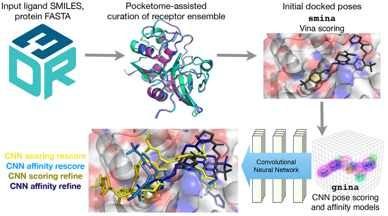
Our general workflow is shown in Figure 1. We used a structure-based docking and scoring approach, with pose sampling fundamentally based on the Autodock Vina scoring function as implemented in smina [28], a fork of the original project with increased support for minimization and custom scoring function development. We used our CNN scoring function to both further refine and simply rescore the poses generated by docking with smina, using the CNN affinity prediction and pose score as the basis for distinct submissions. This yielded a minimum of four unique CNN-based submissions for each subchallenge. We compare to smina’s performance to test whether the CNN model is capable of improving on the accuracy of an existing scoring model, and independently evaluate the performance of the affinity and scoring outputs, as well as the CNN’s ability to score putative binding modes and sample those modes itself.

Fig. 1:

Workflow used to produce gnina convolutional neural network-based predictions for binding poses and binding affinity rankings.

D3R Grand Challenge 3 consisted of five subchallenges, the first of which consisted of three phases. Only the multiphase subchallenge 1 involved a pose prediction component, while all subchallenges involved predicting affinities and/or affinity rankings. Subchallenge 1, for which the target was Cathepsin S, involved both cross-docking (stage 1A) and redocking (stage 1B) tasks for 24 ligands for which ligand-protein co-crystal structures were available but unreleased until after stage 1B, and predicting affinity rankings for 136 compounds that were a superset of those 24 both before (stage 1A) and after (stage 2) unblinding of the co-crystal structures. The remaining four subchallenges all involved kinases. The stated aim of subchallenge 2 was to test compound selectivity prediction; accordingly, it featured the kinases VEGFR2, JAK2, and p38α and 54 compounds for which K_d values were available for all three of these proteins. Subchallenges 3 and 4 were both designed to test accuracy at predicting large changes in binding affinity due to small changes in compound structure; in subchallenge 3 the target was again JAK2 and it involved 17 congeneric compounds, while in subchallenge 4 the target was TIE2 and it involved 18 congeneric compounds. Subchallenge 5 was designed to test accuracy at predicting the effect of target protein mutations on compound binding affinity, and its target was the wild type and five mutants of the target ABL1, with only two compounds. Subchallenges 2–4 did not specify the phosphorylation state of the target proteins, while subchallenge 5 noted that all proteins were unphosphorylated; we simply used the phosphorylation state of the reference receptors chosen from the PDB. Subchallenge 3 noted that chiral compounds were measured as a racemic mixture, and so for this subchallenge we docked all enantiomers of each compound.

2.1. CNN Training

Our architecture, input format, and training approach have been described previously [57–59]. Briefly, we designed a four-dimensional grid-based input representation consisting of a vector of spatially distributed atom densities for each supported atom type, where atom types fundamentally distinguish between protein and ligand atoms, different elements, and the protonation states of those atoms. The density of a particular atom within its relevant atom channel is represented as a piecewise continuous function g(d, r), where d is the distance from the atom center and r is the van der Waals radius:

$$g(d,r)=\{\begin{array}{ll}{e}^{-\frac{2d^2}{r^2}}\hfill & 0\le d<r\hfill \\ \frac{4}{e^2{r}^2}{d}^2-\frac{12}{e^{2}r}d+\frac{9}{e^2}\hfill & r\le d<1.5r\hfill \\ 0\hfill & d\ge 1.5r\hfill \end{array}$$ (1)

The CNN maps its input to an output value that is either a probability distribution over class labels (i.e.whether or not a given input is a binding pose) or a real-valued affinity prediction. The architecture used during D3R GC3 can be found in Figure 2.

Fig. 2:

Architecture of the neural network used to rescore and refine poses. The input is a voxelized grid of Gaussian atom type densities.

The CNN was trained using poses generated by redocking the 2016 PDBbind refined set [61] using the Autodock Vina scoring function as implemented in smina. Poses within 2Å RMSD are labeled as actives for the binary classification output and given the binding affinity as the target value for the regression output, while all other poses are labeled as inactives for the purposes of binary classification and are penalized (via a hinge loss) only if the predicted affinity is too high. In order to increase the number of active examples in the training set, these docked poses were supplemented with crystal poses minimized using the Autodock Vina scoring function. The training set was then further expanded by performing three rounds of iterative training during which a model was trained, used to refine the docked poses, and then the poses resulting from that process labeled based on the crystal structure and added to the training set for the next round. Using this training set of 250,000 poses, the final model was trained for 150,000 iterations with a batch size of 50 using our customized version of the GPU-optimized Caffe [62] deep learning framework. Each batch was balanced to contain an equal number of positive and negative examples (low and high RMSD poses) as well as stratified by receptor so that every receptor target was uniformly sampled, regardless of the number of docked structures. At each iteration, a random rotation and translation was applied to every input complex in order to prevent the network from learning coordinate-frame dependent features.

2.2. Pose Generation

The basic information provided for each subchallenge consisted of SMILES for the relevant compounds and FASTA sequences for the relevant proteins. RDKit [63] was used to generate a three-dimensional conformer based on the provided SMILES for each compound; only one conformer was required (or one conformer per enantiomer in subchallenge 3) because the conformational space of the ligand was subsequently explored during docking. Each protein was used to query Pocketome [64] for relevant PDB accession IDs. All available holo structures were aligned and visually inspected to manually select a conformationally diverse subset of reference structures for docking. Table 1 shows the PDB accession IDs for the reference structures that were chosen. The IDs associated with ABL1 include 1FPU, 1OPJ, and 2G1T (used as references for the wild type protein and also point-mutated in PyMOL[65] as references for the F317I, F317L, and Q252H mutations); 2G2F, 2G2H, and 2G2I (references for the H396P mutation); and 2V7A (reference for the T315I mutation). The generated conformers for each compound were then docked into the corresponding reference receptor ensemble using Vina; an additional set of docked poses was generated by performing the final minimization of the poses sampled by Vina during the Monte Carlo routine with the CNN pose scoring layer (“CNN refinement”) - this is a hybrid technique where the fast Vina scoring is used for the Metropolis criterion during Monte Carlo sampling and the slower CNN scoring is only used to minimize ligand poses selected by the sampling. The Vina docked poses were then rescored using both the CNN scoring and affinity layers, and the CNN refined poses were also rescored using the CNN affinity layer. Ranking the poses by score thereby produces a maximum of five predictions per subchallenge, although CatS phase1B (the redocking subchallenge) featured ten submissions due to redocking either with crystal waters present or absent. The top five poses for each method were submitted for the pose prediction tasks, while scoring tasks utilized the top-scoring pose for each compound to make the scoring prediction and compound ranking. Vina’s predictions were only submitted for CatS; for the other targets only the CNN-based predictions were officially submitted, though we show the results of Vina scoring for comparison in the ensuing analysis. Furthermore, we also show our results for ABL1 (subchallenge 5) using the same methods as were used in the rest of the challenge, although the required calculations were completed after the end of the challenge period.

Table 1:

Targets that appeared in at least one of the subchallenges of D3R Grand Challenge 3, with the PDB IDs used as references for docking; the most similar target in the PDBbind 2016 refined set, used to train the CNN, with its similarity to the provided FASTA sequence for the D3R target; mean and maximum Tanimoto coefficient of the crystal ligand associated with the PDBbind refined set target to the compounds in the challenge.

Target	reference PDB IDs	PDBbind/similarity	mean/max Tanimoto
CatS	2F1G, 2HXZ 2G7Y,3KWN 2HHN	2HHN/0.991	0.209/0.256
JAK2(SC2)	2W1I, 3E62 3JY9, 3UGC 4AGC, 5I4N 5UT2, 5UT5 5UT6	4JIA/0.980	0.291/0.437
VEGFR2	1VR2, 1YWN 2OH4, 2P2H 2P2I, 2GU5 3B8R, 3VNT	4ASE/0.657	0.214/0.414
p38α	1M7Q, 1OVE 1W82, 1W83 1WBS, 2GHL 2ZB1, 3ITZ 3L8S, 3NNU	1YQJ/0.978	0.278/0.488
JAK2(SC3)	2W1I, 3E62 3JY9, 3UGC 4AGC, 5I4N 5UT2, 5UT5 5UT6	4JIA/0.980	0.357/0.413
TIE2	2OO8, 2OSC 2P4I, 2WQB 3L8P, 4X3J	4V01/0.482	0.239/0.363
ABL1	1FPU, 1OPJ 2G1T,2G2F 2G2H,2G2I 2V7A	3K5V/0.979	0.302/0.332

3. Results

General information about the targets used in D3R GC3 is found in Table 1, including the aforementioned PDB IDs used to produce binding poses as well as basic measures of the similarity of the challenge targets and compounds to their most comparable targets and compounds used in the training set. In particular, the third column shows the PDB accession ID of the target in the training set that has highest sequence similarity to each GC3 target, and the fourth column shows the mean and maximum Tanimoto coefficient for that target’s co-crystal ligand to the accompanying GC3 tar get’s compounds. Tanimoto coefficients were calculated using OpenBabel [66] with FP2 fingerprints. Notably, while the most similar target to TIE2 does not have high global sequence similarity compared with the other D3R targets and their most similar training set target, it is FGFR1, whose catalytic domain is known to be highly similar to TIE2[67]. From these data we can conclude that while our training data included at least one target that was highly similar to each of the GC3 targets, the associated poses used for training did not include compounds that were particularly similar to the GC3 compounds; therefore GC3 may serve as a fair test of the CNN’s generalization ability.

3.1. Pose Prediction

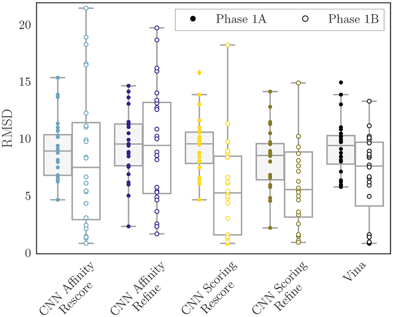
The GC3 pose prediction task was limited to a 24 compound subset of the Cathepsin S subchallenge. Participants were asked to provide predicted binding poses without (stage 1A) and with (stage 1B) knowledge of the cognate receptor structure for each compound. Up to five poses could be submitted. To maintain an automated and general approach for the submission, we produced poses by docking into a diverse receptor ensemble, using the entire binding site as the search space. Figure 3 shows the RMSD of the best pose submitted per compound for each scoring method, grouped by the method and showing the RMSD distribution for each challenge stage. The following statistics are computed based on the best-submitted pose per compound. The method associated with the lowest mean RMSD among all our submissions in stage 1A was using the CNN pose scoring model to rescore Vina-generated docked poses (“CNN Scoring Rescore”); its mean RMSD was 8.35Å and its rank among all submissions based on the mean RMSD was 31/44. The method associated with the lowest median RMSD among all our submissions in stage 1A was using the CNN pose scoring model to refine poses sampled by Vina during the Monte Carlo search (“CNN Scoring Refine”); its median RMSD was 8.16Å and its rank among all submissions based on the median RMSD was 31/44. The method associated with the lowest mean and median RMSD among all our submissions in stage 1B was using the CNN pose scoring model to rescore Vina-generated docked poses; its mean RMSD was 9.70Å and its rank among all submissions based on the mean RMSD was 23/47. Its median RMSD was7.33Å and its rank among all submissions based on the median RMSD was 13/47.

Fig. 3:

Per-compound best RMSDs for each method’s submissions in stage 1A (cross-docking, left) and stage 1B (redocking, right). Pose prediction submissions consisted of the top 5 poses according to each scoring method.

3.1.1. Sampling

Our CatS pose prediction performance was generally poor, even when redocking. A pose within 2.5Å RMSD was sampled for only a third of the test compounds. Nine poses were sampled per ligand, per reference receptor, resulting in 45 poses per ligand in stage 1A and 18 poses per ligand in stage 1B. Redocking in particular was characterized by high variance in the best-predicted RMSDs across the set of test compounds. Docking into the large CatS binding site using our scoring methods yielded predictions that were distributed throughout the search space, but in reality binding appears to be localized to a specific region.

Figure 4 shows the center of mass locations for available reference structures and for our top-ranked predictions. The GC3 compounds are densely clustered in one region of the pocket, while the available experimental data from the PDB support a somewhat larger binding region (and potentially more diverse binding modes). However, both Vina and the CNN produced many high-ranking poses that appeared in a different region of the pocket altogether. In particular, when docking with water using Vina the average distance to the closest center of mass in the set of D3R ligands is 8.11Å, and the average distance to the closest center of mass in the set of reference receptor ligands is 6.00Å; when using the CNN for the final refinement the average distance to the closest center of mass in the set of D3R ligands is5.00Å, and the average distance to the closest center of mass in the set of reference receptor ligands is 3.97Å. When docking without water using Vina the average distance to the closest center of mass in the set of D3R ligands is 4.01Å, and the average distance to the closest center of mass in the set of reference receptor ligands is 2.48Å; when using the CNN for the final refinement the average distance to the closest center of mass in the set of D3R ligands is 3.18Å, and the average distance to the closest center of mass in the set of reference receptor ligands is 2.22Å. Thus both methods produced on average more poses in the region of the pocket where the GC3 ligands actually bind when docking without crystal waters, but the CNN was better in both cases at generating as top-ranked poses those that were closer to the general region of the pocket where the crystal ligands appear.

Fig. 4:

Center of mass locations for the unblinded crystal poses of the GC3 CatS co-crystal ligands (green), the co-crystal ligands of the reference PDB structures used during phase 1 docking (blue), and the highest ranked docked poses for each compound generated by redocking (the stage 1B task) with Vina (gray), and CNN refinement (gold). The left subfigure shows the results from docking with crystal waters present, while the right subfigure shows the results from docking without them.

While docking without crystal waters present resulted in more poses in the general region of the pocket where the GC3 ligands bind, when low RMSD poses (here defined as those within 2.5Å) were sampled, they were most often produced by docking and refinement that utilized the crystal waters. Table 2 shows all 28 of the low RMSD poses sampled by any docking method for both stage 1A (the cross-docking task) and stage 1B (the redocking task). Rows are grouped by compound ID and sorted internally by the pose RMSD to the crystal pose. Values that are not relevant in a particular column are indicated with N/A; specifically, no waters were used during cross-docking and therefore the solvent category is N/A for poses sampled during that task, and the Vina score is N/A for poses generated by the CNN scoring model refinement method.

Table 2:

Poses generated for CatS compounds that were within 2.5Å RMSD of the crystal pose. Colors differentiate cross-docking (brown) from redocking (black); poses produced by Vina alone (black) or with CNN refinement (purple); with solvent (blue) or without (pink); and poses that were ranked in the top 5 (green) or outside of the top 5 (black). Entries are marked as N/A if they do not apply for a specific row (solvent columns for cross-docked poses and Vina’s rank for CNN-generated poses) and they are colored peach to reduce their visual impact.

Compound ID	cross-docking/redocking	RMSD (Å)	generation method	solvent	Vina rank	CNN scoring rank	CNN affinity rank
CatS 5	re	1.463	Vina	water	4	1	2
CatS 5	re	1.745	CNN refine	water	N/A	7	4
CatS 5	cross	1.743	CNN refine	N/A	N/A	15	18
CatS 5	cross	1.976	CNN refine	N/A	N/A	24	26
CatS 5	re	2.257	Vina	water	11	2	3
CatS 5	re	2.498	CNN refine	water	N/A	6	5
CatS 10	cross	2.272	CNN refine	N/A	N/A	2	11
CatS 11	re	1.362	Vina	water	11	1	4
CatS 15	re	0.915	Vina	water	1	1	2
CatS 15	re	1.166	CNN refine	water	N/A	4	8
CatS 15	cross	1.436	CNN refine	N/A	N/A	26	15
CatS 15	cross	2.404	CNN refine	N/A	N/A	13	3
CatS 16	re	0.989	Vina	water	2	1	6
CatS 16	re	1.522	CNN refine	water	N/A	1	6
CatS 16	re	1.535	Vina	water	10	2	5
CatS 16	re	1.768	Vina	water	14	5	12
CatS 16	re	2.072	CNN refine	water	N/A	7	12
CatS 16	re	2.254	Vina	water	1	3	6
CatS 16	re	2.388	CNN refine	water	N/A	3	3
CatS 17	re	1.599	Vina	water	1	2	10
CatS 17	re	1.643	CNN refine	water	N/A	3	15
CatS 17	re	1.762	CNN refine	water	N/A	1	14
CatS 20	re	1.679	Vina	water	2	1	13
CatS 20	re	1.691	CNN refine	water	N/A	2	15
CatS 20	re	2.005	CNN refine	no water	N/A	14	10
CatS 20	re	2.217	Vina	no water	5	8	4
CatS 24	re	0.998	CNN refine	water	N/A	2	10
CatS 24	re	1.043	Vina	water	1	1	8

Significant categorical features are highlighted, including: cross-docking versus redocking; poses produced by full Vina docking versus Vina Monte Carlo sampling followed by refinement with the CNN scoring model; crystal waters used or removed; and rank among all of that compound’s poses scored by a particular method, with any rank within the top five highlighted. The CNN scoring model was used to both rescore Vina’s poses and produce its own refined poses, and the CNN affinity model was used to rescore both Vina’s docked poses and the CNN refined poses. Consequently, these methods have two associated sets of rankings for each compound, which correspond to separate submissions to the challenge; they may therefore have up to two poses at any given rank in the table. Additionally, poses generated by docking with and without waters are grouped together to produce the ranking shown in the table; the effect of solvent will be explored in greater detail in section 3.1.3.

Only 8/24 compounds had any pose within 2.5Å RMSD of the crystal pose; only 3 had a low-RMSD pose sampled during the cross-docking task, while 7 had a low-RMSD pose sampled during redocking. It is notable that all five low-RMSD poses generated during the cross-docking task were produced by using the CNN for final refinement, though these poses were ranked in the top five only twice, once by the CNN scoring model (which sampled them) and once by the CNN affinity model (which re-scored them). CNN refinement outperformed Vina for only one compound during the redocking task (CatS 24), though it produced nearly as many low-RMSD poses (11 poses to Vina’s 12). Though the CNN’s sampling was guided at a coarse-grained level by Vina, which was used during Monte Carlo sampling, it is worth noting that in most cases its refinement did not move “good” poses in such a way that they were no longer “good” according to our threshold, and that in a few cases the CNN appears to have succeeded in moving a pose closer to the crystal pose than Vina did, as evidenced by succeeding in sampling a good pose during stage 1A, by improving on the best Vina pose RMSD, or by producing more low-RMSD poses than Vina did. Examples of cases where the CNN improved on a Vina pose (as shown in Table 2) include CatS 5, CatS 10, CatS 15, CatS 17, CatS 20, and CatS 24. A notable exception is CatS 11; only Vina sampled a low RMSD pose for that compound.

3.1.2. Rescoring

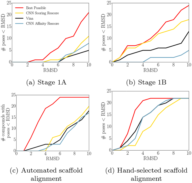
Vina and the CNN combined only sampled a low-RMSD pose for a third of the CatS compounds. When Vina sampled a low-RMSD pose during the challenge, the CNN scoring model was more likely than either Vina or the CNN affinity model to identify it as the top-ranked prediction for the associated compound. Fig 5 shows the best possible performance given the poses sampled with Vina (red lines), and then shows how significantly each scoring model deviated from that performance in its selection of top-ranked poses.

Fig. 5:

Number of poses within a given RMSD that can be found as a top-ranked pose using Vina or re-scoring Vina-generated poses with the CNN scoring or affinity models for CatS stage 1A (a), stage 1B (combining poses sampled with and without solvent) (b), and two ligand similarity-based methods ((c) and (d)). The performance that would be attained if the sampled pose with the lowest RMSD were selected as the top pose is shown in red.

The CNN scoring model outperforms the other models when using the receptor ensemble approach utilized during the challenge as well as when performing redocking. The CNN’s improved performance on stage 1A, in Figure 5a, is marginal; the CNN scoring model appears to be the only method to feature a top-ranked pose within 5Å RMSD when choosing among the poses sampled by Vina. Figure 5b, showing stage 1B performance, is more unequivocal, with the CNN scoring model nearly matching the best possible performance for low RMSD poses while the other methods fail to identify several available low-RMSD poses.

Figures 5c and 5d show new analyses performed after the subchallenge ended; they utilize preexisting experimental data to guide pose prediction. The available PDB structures of CatS were queried to identify the crystal ligand with the highest Tanimoto coefficient with each GC3 compound, and the GC3 compound was then aligned by scaffold to that crystal ligand using up to 100 conformers. In (c) the scaffold was chosen by generating a Murcko decomposition of each query and reference compound and the maximum common substructure of these were aligned; in (d) the scaffolds were chosen by visual inspection. The aligned poses were then minimized and rescored according to the same procedure used to sample and rescore poses for the original submissions, and the compounds were also cross-docked into a box defined by the binding pose of the chosen reference. This method is less general than docking agnostically into regions of the pocket, since it relies on information about similar ligands being available, but it produces significantly improved pose prediction performance in this case. Using this procedure for sampling, Vina outperforms the CNN at identifying available low-RMSD poses, though all methods fail to approach the “best available” performance.

3.1.3. Solvent effects

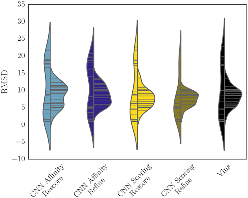
Redocking in stage 1B, for which crystal waters were available, affords an opportunity to examine whether Vina and the CNN scoring models differ in their abilities to correctly rank poses generated with and without crystal waters. Figure 6 shows the RMSD of the best pose submitted per-compound using each method. Including solvent increases the variance in the best predicted RMSDs, producing an apparently bimodal distribution with peaks at both lower and higher RMSDs than the medians of the distributions without solvent. The method that used the CNN for both refinement and the final ranking (“CNN Scoring Refine”) may slightly improve on Vina’s performance by both reducing the density at high RMSD when sampling with solvent and by shifting the median toward a slightly lower RMSD when sampling without solvent.

Fig. 6:

Per-compound best RMSDs for each method’s submissions in stage 1B, split between solvent (left) and no solvent (right).

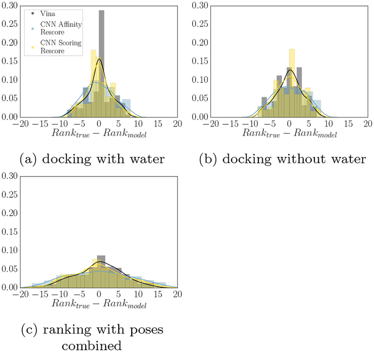
Figure 7 considers how many times a given method provided a pose ranking that deviated from that pose’s true ranking by specific amounts. A perfect classifier would have its entire density at 0, and greater spread corresponds to a less accurate ranking; compared to a correlation metric, this analysis gives information about where ranking deviations occur. All methods have lower standard deviation of their ranking error when ranking poses sampled with solvent than those sampled without it. They also have kurtosis closest to 0 when sampling with solvent - Vina and CNN scoring both have kurtosis around 0 in that case, compared with kurtosis of −0.393 and −0.492 respectively when sampling without solvent, and −0.163 and −0.370 respectively when ranking all poses. CNN scoring is less skewed when ranking poses sampled without solvent than Vina is (−0.026 versus −0.132), which corresponds to making fewer errors in misclassifying high RMSD poses as low RMSD poses. Vina’s skew is consistently negative, with its most negative skew when ranking poses sampled with solvent, while CNN scoring has positive skew when ranking poses sampled with solvent. The CNN affinity model has consistently more negative kurtosis and higher standard deviation than the other two methods, which accords with its generally worse performance at pose prediction.

Fig. 7:

Deviation of pose rankings from their true ranking, for docking with (a) and without (b) water. A classifier is more accurate if it is more strongly peaked around the center; a perfect predictor would have all of its density at 0. Combining poses generated with and without solvent produces (c).

3.1.4. Crystal pose scoring

Since so few low-RMSD poses were sampled, it merits investigating whether our poor CatS pose prediction performance was primarily a sampling problem (potentially due to too large a search space) or whether our scoring methods generally failed to score poses near the crystal pose well when performing sampling in the CatS binding site. To do this, we both re-scored the crystal poses using all three scoring methods and also minimized those poses using Vina and the CNN scoring model, then re-scored the minimized poses with the CNN scoring and affinity models as appropriate.

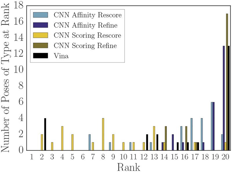
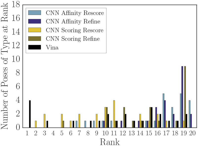
As one measure of the accuracy of a scoring method, we can use the re-scored crystal and minimized crystal poses to determine at which rank they appear when ranking them among the poses sampled during the challenge. Figures 8 (crystal poses) and 9 (minimized crystal poses) show the results of performing that ranking. Vina and the two CNN refinement-based methods rank the crystal poses for over half of the compounds at the lowest position in the ranking (rank 20), while the CNN affinity model rescore of the crystal pose ranked with its rescore of Vina-sampled poses (“CNN Affinity Rescore”) places the crystal poses for over half the compounds in the last three positions of the ranking. In contrast, the CNN scoring model rescore of Vina-sampled poses ranks the crystal poses for 8 compounds in its top 5 poses, and it accounts for over half of the crystal poses by rank 8. Only Vina and the CNN scoring model rank any crystal poses in their top 5 for any of the compounds.

Fig. 8:

Performance of each method at ranking the re-scored crystal poses among all other poses generated during stage 1B and the minimized crystal pose.

Methods were somewhat more likely to place crystal poses minimized with respect to their own scoring function at a high rank than the crystal poses themselves. The CNN refinement method with the scoring model ranking has one such pose in its top 5, and all methods feature at least one minimized crystal pose in their top 10. Vina has more mimimized crystal than crystal poses in its top 5, and their average rank is higher; in contrast the CNN scoring model applied to rescoring Vina’s poses (“CNN Scoring Rescore”) has fewer of Vina’s minimized crystal poses in its top 5 than it had crystal poses, but it ranks half of the compound’s minimized crystal poses in the top 10 compared with Vina’s ranking of half within the top 12.

These figures and the associated underlying data suggest that the CNN scoring model has a slight preference for the true crystal poses over Vina’s minimized crystal poses. Specifically, 8 crystal poses appeared in its top 5 while 5 Vina-minimized crystal poses appeared in its top 5. 10 of those poses were crystal/minimized crystal pairs, with 3 crystals appearing at a higher rank than their minimized partner and 2 minimized poses appearing above their crystal partner; when a minimized pose appeared above the crystal, the average deviation in their ranks was 1, but when a crystal was ranked higher, the average deviation in their ranks was 2.3. The remaining 3 poses were crystal poses for which the corresponding minimized crystal pose appeared outside of the top 5. In contrast, Vina ranks 4 minimized crystals at rank 1, followed by their corresponding crystal poses at rank 2, and then a lone minimized crystal pose at rank 3. However, since CNN refinement generally produced poses even further away from the crystal pose, and the CNN scoring refinement pose generation method mostly ranked those poses over the crystal or minimized crystal poses, it is not the case that the CNN scoring model generally has a global minimum closer to the CatS crystal pose than Vina does; all that appears to be true is that the crystal pose is typically closer to a CNN scoring model minimum or saddle than a Vina-produced pose is. Furthermore, across all models it is true that the crystal pose or the nearest local minimum according to either Vina or the CNN pose scoring model generally do not coincide with the global minimum.

3.1.5. Pose optimization and scoring

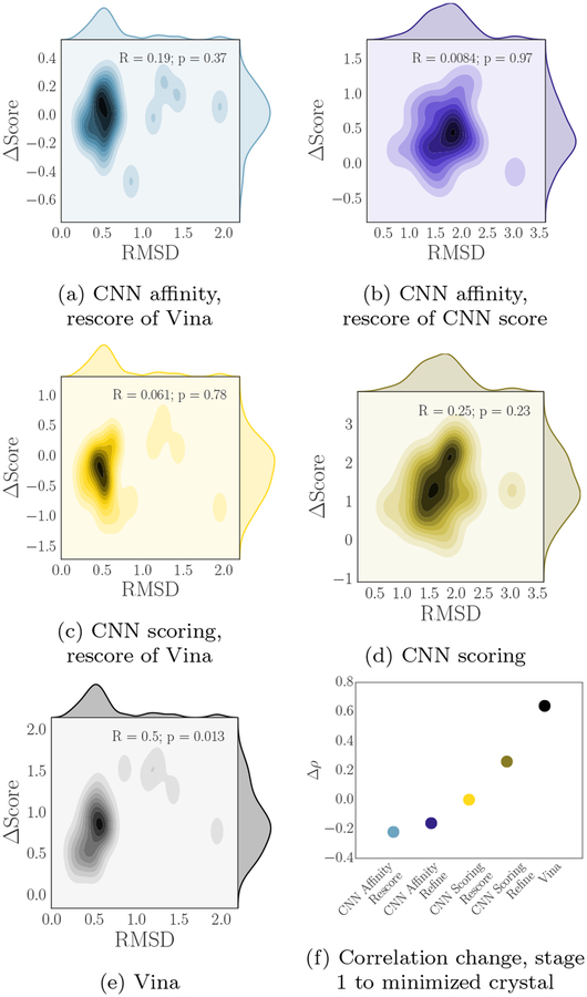
Figure 10 takes a closer look at a projection of the landscape of the three scoring models in the region around the crystal poses for the CatS pose prediction compounds (the CNN scoring model output, which is a probability, has had the logit transform applied). The left column shows the RMSD of the poses produced by minimizing crystal poses with Vina and the change in score associated with the CNN affinity model (10a), CNN scoring model (10c), and Vina (10e). The right column shows the RMSD of the poses produced by minimizing crystal poses with the CNN scoring model and the change in score associated with the CNN affinity model (10b) and the CNN scoring model (10d).

Fig. 10:

(a-e) Change in score vs. change in RMSD for crystal pose minimization, showing differences and correlation (or lack of correlation) in the functional landscape between the different scoring methods. The logit of the CNN score was used to compute ΔScore on the relevant plots. (f) Change in Spearman ρ when scoring with the high RMSD stage 1 CatS poses versus scoring with the minimized crystal poses.

One pattern that emerges is that minimizing with the CNN scoring model (middle right) tends to produce poses that are further from the crystal than Vina does; it also produces a larger range of changes in score, with a distribution that is potentially bimodal, including examples for which it performed comparatively large rearrangements of the input to produce correspondingly large changes in the final score. This does not appear to happen when performing minimization with Vina, suggesting that the CNN scoring model has a smoother landscape, at least around these minima, since it moves a larger distance before converging; alternatively Vina may on average have minima nearer to the crystal pose than the CNN scoring model does, or a combination of both factors may be relevant. Additionally, it is evident that the CNN scoring model is not correlated with Vina, nor is it correlated with the CNN affinity model; the only scoring model relationship that shows any correlation is the CNN affinity model with Vina.

Figure 10f shows a related analysis for crystal pose minimization; challenge stages 1 and 2 involved submitting affinity predictions that were based on poses generated as described. For stage 1 the analysis above demonstrates that these poses were typically far from the true poses, while the process of minimizing the crystal poses produced low-RMSD poses that coincided with a scoring model local minimum for nearly every compound (one compound was minimized to a configuration that was slightly outside of our definition of “low-RMSD” but is still much closer to its crystal pose than the stage 1 poses were). Notably, our submission for stage 1 produced the top-ranked correlation for predicting the affinity rankings of the cocrystal ligand CatS subset among all GC3 submissions, and our overall affinity rankings were also reasonably well-correlated during stage 1 (Table 3). However, in stage 2, with unblinded cocrystal structures available, our affinity prediction performance for CatS actually worsened. Additionally, the method that produced good correlations when predicting affinities for the cocrystal ligand subset was the CNN affinity model, which we do not train to predict poses. Thus we have some reason to suspect that our CNN affinity rankings for CatS are pose insensitive, or at least that whatever aspect of the poses that is useful for predicting affinities is not related to the experimental validity of those poses. Figure 10f shows that while Vina’s affinity prediction correlation significantly improves when using just the minimized crystal poses compared with the random poses from stage 1, and the CNN scoring refinement method improves to a lesser extent, the CNN scoring method that simply rescores Vina’s poses has virtually identical correlation in these two cases (i.e. the poses do not matter) and the two CNN affinity-based methods actually have worse performance when using the correct poses.

Table 3:

The rank of our top-performing CNN method among all submissions to D3R GC3 affinity ranking tasks, along with the Spearman ρ associated with that method, and the Spearman ρ associated with Vina’s predictions. The higher correlation between the best-performing CNN method and Vina’s is bolded. The ABL1 results were not submitted during the challenge period and all official submissions were partials, so we do not show a rank here.

Target	Rank	ρ	Method	Vina
CatS (1a)	6/53	0.37	CNN scoring refine	0.19
JAK2 (SC2)	1/27	0.74	CNN scoring refine	0.05
VEGFR2	14/33	0.39	CNN scoring refine	0.51
p38α	7/29	0.04	CNN scoring refine	−0.34
JAK2 (SC3)	2/18	0.75	CNN affinity refine	−0.33
TIE2	3/18	0.67	CNN affinity rescore	0.14
ABL1	N/A	0.56	CNN affinity rescore/refine (tie)	0.72

3.2. Affinity rankings

Next we consider our performance at producing affinity rankings. Table 3 shows the ranks and Spearman ρ correlations of our best performing CNN models, as well as whether they outperformed Vina according to this metric. We find that the CNN models, particularly CNN scoring, generally outperform Vina at producing scores that correlate with compounds’ true affinity. Additionally, the correlations associated with both JAK2 subchallenges, as well as the TIE2 subchallenge, are relatively strong, and the overall rank of our best submissions for those subchallenges are competitive with others who participated in GC3, as shown in the table’s rank column. It is notable that the best-performing method for two of those three correlated sets of predictions is the CNN affinity model. In contrast, our performance on target p38α in the original challenge was extremely poor.

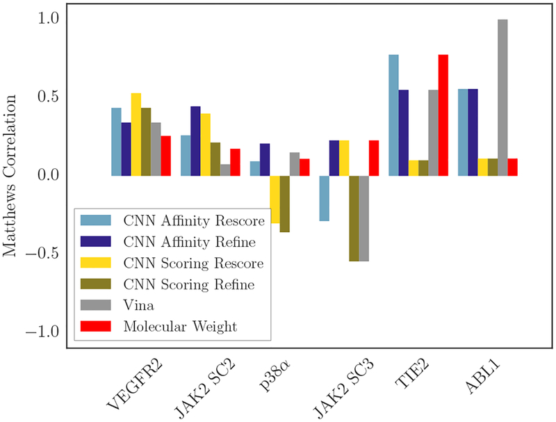
Table 4 shows the ranks and Matthews correlation coefficients in a manner similar to the previous table; this statistic represents performance at binary classification of actives. This analysis suggests that the CNN affinity model has an advantage at active/inactive discrimination when compared with both the CNN scoring model and Vina.

Table 4:

The rank of our top-performing CNN method among all submissions to D3R GC3 affinity ranking tasks based on active/inactive discrimination, along with the Matthews correlation coefficient associated with that method, and the Matthews correlation coefficient associated with Vina’s predictions. The higher correlation between the best-performing CNN method and Vina’s is bolded. The ABL1 results were not submitted during the challenge period and all official submissions were partials, so we do not show a rank here.

Target	Rank	MCC	Method	Vina
JAK2 (SC2)	3/27	0.44	CNN affinity refine	0.07
VEGFR2	1/33	0.53	CNN scoring rescore	0.34
p38α	9/29	0.21	CNN affinity refine	0.15
JAK2 (SC3)	2/18	0.23	CNN affinity refine	−0.55
TIE2	1/17 (tie)	0.78	CNN affinity rescore	0.55
ABL1	N/A	0.56	CNN affinity rescore/refine (tie)	1.00

3.2.1. Correlations

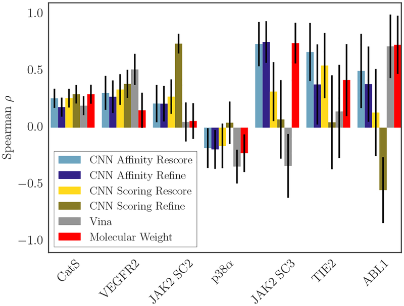
Figure 11 shows the correlations associated with all the methods we used to generate affinity rankings, as well as the correlation that can be obtained by simply using the compounds’ molecular weight (the molecular weight ranking is misleading for target ABL1, since there are only two compounds that have differing affinities for ABL1 mutants, and the molecular weight gives a high correlation here but completely fails at the prediction task for which the challenge was designed).

Fig. 11:

Spearman ρ of each scoring method with the associated experimental data for each target; compounds with K_d ≥10μM have been omitted. Black lines indicate error bars computed by bootstrapping the correlation for 10,000 iterations by resampling data points with replacement. For the bootstrapped correlations, the experimental data was perturbed with randomly generated Gaussian noise $ϵ~\mathcal{N}\left(0,RT\text{ ln}\left(I_{err}\right)\right)$, where I_err was taken to be 2.5.

There is no one method that performs well across all targets. The CNN scoring model is the top-performing method on one of the JAK2 subchallenges, while the CNN affinity model is the top-performing method on the other, and for each method it is the case that in the subchallenge for which they are not the top-ranked method, they actually perform very poorly. From this figure, it is not clear whether the CNN affinity or CNN scoring model is better-suited to performing the affinity ranking task; each performed well on half of the targets shown here, and the targets on which one method performed well preserve the pattern seen with JAK2 - one CNN model having highly correlated scores for a target is mutually exclusive with respect to the other CNN model.

Similarly, Figure 12 shows the Matthews correlation coefficients associated with all the methods used to generate affinity rankings for each target for which this analysis is appropriate, as well as the correlation obtained by using molecular weight. It again suggests that the CNN affinity model has an advantage at active/inactive classification over the other methods, where it is the best-performing method on four of the targets and comparable to the best-performing method on another; here its consistent good performance is unique among the discrimination methods used.

Fig. 12:

Matthews correlation coefficient of each scoring method with the associated experimental data for each target. The K_i compounds with K_d ≥10μM were taken as inactive, and the corresponding K_i bottom-ranked compounds for each prediction method were also taken as inactive. The remaining compounds in both cases were taken as active, and the resulting set of true/predicted pairs were used to compute the correlation. Error bars are not shown as this procedure is not amenable to bootstrapped error estimates.

3.2.2. AUCs

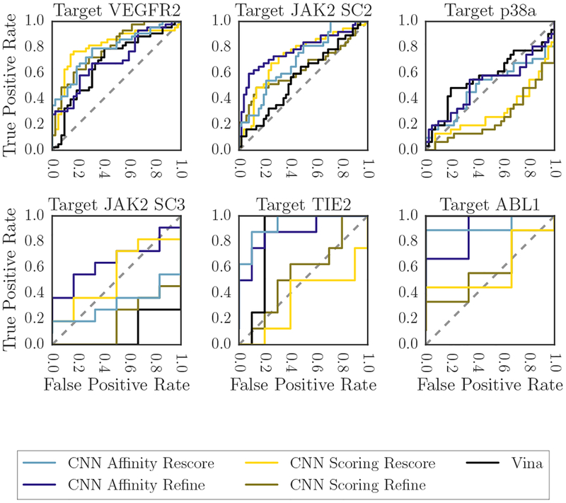
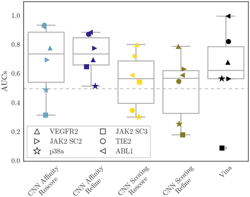
As an alternative view of the CNN ranking performance, Figure 13 shows the per-target ROC plots for the six subchallenges that had compounds with affinities both above and below 10μM, with affinities at or above that point being considered inactive and affinities below that point considered active. Figure 14 instead shows box-plots of the AUCs derived from the ROC plots in Figure 13. In this binding discrimination task, the CNN affinity model is clearly better than the CNN scoring model, and it is generally better than Vina as well, especially when the poses it is scoring were produced via refinement with the CNN scoring model.

Fig. 13:

ROC curves for all GC3 targets for which there were compounds with K_d ≥ 10μM and compounds with K_d < 10μM; the former were considered inactive and the latter active for the purposes of this figure.

Fig. 14:

Boxplots of AUCs across all methods and GC3 targets for which there were compounds with K_d ≥ 10μM and compounds with K_d < 10μM; the former were considered inactive and the latter active for the purposes of this figure.

3.2.3. Ligand similarity-based retrospective

Since we did not use ligand similarity between prediction compounds and available reference structures to identify possible binding modes during the challenge, we considered whether using this information would have been beneficial when producing affinity rankings (particularly on the targets for which we performed poorly). To that end, we utilized the approach described in section 3.1.2 to perform alignment, minimization, and docking based on the available reference structure whose crystal ligand had highest similarity to each query compound.

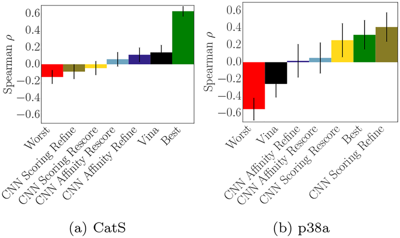
The results of this approach on pose prediction were shown in Figure 5c and Figure 5d, while its effect on the correlation of the final scores (when taking the top-ranked prediction for each compound as its predicted affinity) is shown for CatS in Figure 15a (which shows the correlation produced by the same method used to generate 5d). In general, when using our current scoring functions for CatS, methods that produce better poses also produce worse correlation for the predicted affinities - for example, our original stage 1A Spearman ρ was 0.37, while the ligand-similarity based method shown in 5d and 15a had a best-case Spearman ρ of 0.14.

Fig. 15:

Performing the scoring and affinity ranking process again using ligand structural information for(a) CatS and (b) p38α. The best and worst overall submissions from the original challenge are shown with the new results. Using this process, we had worse performance on predicting CatS affinity rankings but much better performance on p38α.

We also performed this analysis to generate new predictions for p38 using ligand similarity. The best correlation produced by that analysis is shown in Figure 15b. This method produced good correlation using the CNN scoring model, particularly when the scoring model was used to sample poses itself in the final refinement. Notably, these results were dependent on the method used to identify similar ligands as well as the alignment method; for CatS, Tanimoto distance computed with OpenBabel FP2 fingerprints and a scaffold alignment (using the hand-selected scaffold) produced the best results for pose prediction (though no similarity-based method we tried produced correlation that matched our original stage 1 submission), while for p38α the best result was produced using a Tanimoto distance computed with RDKit Daylight-like fingerprints and O3A shape alignment.

4. Discussion

The 2017 D3R Grand Challenge presented diverse subchallenges spanning several classes of problems in computational chemistry. There was one pose prediction component that ultimately encompassed both redocking and cross-docking for a single target, and several affinity prediction/ranking components that were constructed to test binding discrimination and affinity prediction in different contexts. We used this opportunity to evaluate the convolutional neural network-based scoring functions we have been developing, particularly recent work that enables us to use the CNN to optimize input poses. We found that although our performance was best-in-class when performing affinity ranking for two of the targets (three of the subchallenges), our performance was average on two of the other targets and poor on a third. Additionally, our performance at pose prediction was limited not only by inadequate sampling, but also by failures of both Vina and the CNN to identify crystal and near-crystal poses as high-ranking poses when they are sampled. In both cases poor performance at ranking is partially due to mistakenly identifying other poses that are actually far from the crystal pose as being better, though we have not yet identified the causes of these failures. However, when using the CNN to rescore poses generated by Vina, the CNN was in some cases much better than Vina at correctly ranking low-RMSD poses. It also exhibited some promising signs when guiding sampling itself; it sampled several low-RMSD poses during CatS cross-docking, when Vina did not sample any, and also sampled a low-RMSD pose for CatS 10 during redocking when Vina failed to do so, though the reverse is true for CatS 11.

We see a general trend in the CNN performance that accords with what we have previously observed, which is that we often “get what we train for.” Specifically, the CNN scoring model is a relatively effective predictor of low RMSD structural poses, while the CNN affinity model has indifferent performance at this task; conversely the CNN affinity model may have a slight advantage when it comes to discriminating between active and inactive compounds for a given target, as evidenced by the Matthews correlation (Table 4 and Figure 12), ROC curves (Figure 13), and associated AUCs (Figure 14), though the CNN affinity and scoring models both produced scores that correlate with the experimental affinities on some tasks and failed on others. Additionally, the differing performance between Vina and the CNN when performing redocking with and without crystal waters present might be related to the zero-node relevance analysis we have conducted [59], which suggests that the CNN may be implicitly interpreting empty regions in the input as containing solvent. This may enable the CNN to outperform Vina in the absence of explicit solvent, though further analysis is required to understand this phenomenon. More fundamental differences exist between the functional landscapes of Vina and the CNN, as evidenced by our simple projections in the regions around the crystal pose. Since we would like to achieve rapid convergence to a minimum, the CNN’s tendency to make large movements that also significantly improve a pose’s score is actually a desirable property (compared with Vina’s smaller changes to optimize the input); however, this property is only useful if the movements are actually bringing the input closer to the true global minimum, which is still frequently not the case for the CNN.

All our methods appear to have difficulty with CatS in particular, and although we can use reasonable, automated approaches to generate either low-RMSD poses or reasonably correlated affinity predictions for this target, we have not yet found a single method that can do both simultaneously in this case. This suggests that something about its binding modes is represented poorly by our current models and merits further investigation. The CNN appears to have additional issues, since it performs significantly worse than Vina at pose prediction when using the alignment-and-minimization approach taken in Figure 5c and Figure 5d, but was able to identify low-RMSD docked poses during stage 1b (Figure 5b). Since we have not explicitly trained for cross-docking, perhaps it has more difficulty identifying a ligand’s pose as being similar to a binding pose when it is in a foreign binding site, as in the ligand similarity-based analysis. We are currently training to improve cross-docking performance, so we will be able to test whether our performance on this task improves with such training. Ultimately we hope that further interrogation of our performance on D3R GC3 will help us achieve even better performance when we apply the CNN to prospective drug discovery tasks in the future.

Fig. 9:

Performance of each method at ranking the minimized crystal pose among all other poses generated during stage 1B and re-scored crystal pose.

References

- 1.Wang Jui-Chih and Lin Jung-Hsin. Scoring functions for prediction of protein-ligand interactions. Current pharmaceutical design, 19(12):2174–2182, 2013. [DOI] [PubMed] [Google Scholar]
- 2.Colwell Lucy J. Statistical and machine learning approaches to predicting protein-ligand interactions. Current opinion in structural biology, 49: 123–128, 2018. [DOI] [PubMed] [Google Scholar]
- 3.Braga Rodolpho C, Alves Vinicius M, Silva Arthur C, Nascimento Marilia N, Silva Flavia C, Liao Luciano M, and Andrade Carolina H. Virtual screening strategies in medicinal chemistry: the state of the art and current challenges. Current topics in medicinal chemistry, 14(16):1899–1912, 2014. [DOI] [PubMed] [Google Scholar]
- 4.Javier Pérez-Sianes, Horacio Pérez-Sánchez, and Fernando Díaz. Virtual screening: a challenge for deep learning. In 10th International Conference on Practical Applications of Computational Biology & Bioinformatics, pages 13–22. Springer, 2016. [Google Scholar]
- 5.Sliwoski Gregory, Kothiwale Sandeepkumar, Meiler Jens, and Lowe Edward W. Computational methods in drug discovery. Pharmacological reviews, 66(1):334–395, 2014. [DOI] [PMC free article] [PubMed] [Google Scholar]
- 6.Jansen Johanna M, Amaro Rommie E, Cornell Wendy, Tseng Y Jane, and Walters W Patrick. Computational chemistry and drug discovery: a call to action. Future medicinal chemistry, 4(15):1893–1896, 2012. [DOI] [PubMed] [Google Scholar]
- 7.Boutros Paul C, Margolin Adam A, Stuart Joshua M, Califano Andrea, and Stolovitzky Gustavo. Toward better benchmarking: challenge-based methods assessment in cancer genomics. Genome biology, 15(9):462, 2014. [DOI] [PMC free article] [PubMed] [Google Scholar]
- 8.Gathiaka Symon, Liu Shuai, Chiu Michael, Yang Huanwang, Jeanne A Stuckey You Na Kang, Delproposto Jim, Kubish Ginger, Dunbar James B, Carlson Heather A, et al. D3r grand challenge 2015: evaluation of protein–ligand pose and affinity predictions. Journal of computer-aided molecular design, 30(9):651–668, 2016. [DOI] [PMC free article] [PubMed] [Google Scholar]
- 9.Gaieb Zied, Liu Shuai, Gathiaka Symon, Chiu Michael, Yang Huanwang, Shao Chenghua, Feher Victoria A, Walters W Patrick, Kuhn Bernd, Rudolph Markus G, et al. D3r grand challenge 2: blind prediction of protein–ligand poses, affinity rankings, and relative binding free energies. Journal of computer-aided molecular design, 32(1):1–20, 2018. [DOI] [PMC free article] [PubMed] [Google Scholar]
- 10.José Jiménez Luna, Miha, Gerard Martinez-Rosell, and Gianni De Fabritiis. K deep: Protein-ligand absolute binding affinity prediction via 3dconvolutional neural networks. Journal of chemical information and modeling, 2018. [DOI] [PubMed] [Google Scholar]
- 11.Mobley David L, Graves Alan P, Chodera John D, McReynolds Andrea C, Shoichet Brian K, and Dill Ken A. Predicting absolute ligand binding free energies to a simple model site. Journal of molecular biology, 371(4):1118–1134, 2007. [DOI] [PMC free article] [PubMed] [Google Scholar]
- 12.Aldeghi Matteo, Heifetz Alexander, Bodkin Michael J, Knapp Stefan, and Biggin Philip C. Accurate calculation of the absolute free energy of binding for drug molecules. Chemical science, 7(1):207–218, 2016. [DOI] [PMC free article] [PubMed] [Google Scholar]
- 13.Stjernschantz Eva and Oostenbrink Chris. Improved ligand-protein binding affinity predictions using multiple binding modes. Biophysical journal, 98(11):2682–2691, 2010. [DOI] [PMC free article] [PubMed] [Google Scholar]
- 14.Kim Ryangguk and Skolnick Jeffrey. Assessment of programs for ligand binding affinity prediction. Journal of computational chemistry, 29(8):1316–1331, 2008. [DOI] [PMC free article] [PubMed] [Google Scholar]
- 15.Ashtawy Hossam M and Mahapatra Nihar R. A comparative assessment of ranking accuracies of conventional and machine-learning-based scoring functions for protein-ligand binding affinity prediction. IEEE/ACM Transactions on computational biology and bioinformatics, 9(5):1301–1313, 2012. [DOI] [PubMed] [Google Scholar]
- 16.Carlson Heather A. Lessons learned over four benchmark exercises from the community structure–activity resource, 2016. [DOI] [PMC free article] [PubMed]
- 17.Smith Richard D, Damm-Ganamet Kelly L, Dunbar James B Jr, Ahmed Aqeel, Chinnaswamy Krishnapriya, Delproposto James E, Kubish Ginger M, Tinberg Christine E, Khare Sagar D, Dou Jiayi, et al. Csar benchmark exercise 2013: evaluation of results from a combined computational protein design, docking, and scoring/ranking challenge. Journal of chemical information and modeling, 56(6):1022–1031, 2015. [DOI] [PMC free article] [PubMed] [Google Scholar]
- 18.Carlson Heather A, Smith Richard D, Damm-Ganamet Kelly L, Stuckey Jeanne A, Ahmed Aqeel, Convery Maire A, Somers Donald O, Kranz Michael, Elkins Patricia A, Cui Guanglei, et al. Csar 2014: a benchmark exercise using unpublished data from pharma. Journal of chemical information and modeling, 56(6):1063–1077, 2016. [DOI] [PMC free article] [PubMed] [Google Scholar]
- 19.Harder Edward, Damm Wolfgang, Maple Jon, Wu Chuanjie, Reboul Mark, Jin Yu Xiang Lingle Wang, Lupyan Dmitry, Dahlgren Markus K., Knight Jennifer L., Kaus Joseph W., Cerutti David S., Krilov Goran, Jorgensen William L., Abel Robert, and Friesner Richard A.. OPLS3: A force field providing broad coverage of drug-like small molecules and proteins. J. Chem. Theory Comput, 12(1):281–296, January 2016. doi: 10.1021/acs.jctc.5b00864. URL 10.1021/acs.jctc.5b00864. [DOI] [PubMed] [Google Scholar]
- 20.Yin Shuangye, Biedermannova Lada, Vondrasek Jiri, and Dokholyan Nikolay V.. MedusaScore: An accurate force field-based scoring function for virtual drug screening. Journal of Chemical Information and Modeling, 48(8):1656–1662, August 2008. doi: 10.1021/ci8001167. URL 10.1021/ci8001167. [DOI] [PMC free article] [PubMed] [Google Scholar]
- 21.Case DA, Cheatham TE, Darden T, Gohlke H, Luo R, Merz KM, Onufriev A, Simmerling C, Wang B, and Woods RJ. The Amber biomolecular simulation programs. J. Comput. Chem, 26(16):1668–1688, 2005. ISSN 1096-987X. [doi: 10.1002/jcc.20290]. [DOI] [PMC free article] [PubMed] [Google Scholar]
- 22.Cheng T, Li X, Li Y, Liu Z, and Wang R. Comparative assessment of scoring functions on a diverse test set. J Chem Inf Model, 49(4):1079–93, 2009. [doi: 10.1021/ci9000053]. [DOI] [PubMed] [Google Scholar]
- 23.Ewing TJ, Makino S, Skillman AG, and Kuntz ID. DOCK 4.0: search strategies for automated molecular docking of flexible molecule databases. J Comput Aided Mol Des, 15(5):411–28, 2001. [DOI] [PubMed] [Google Scholar]
- 24.Brooks BR, Bruccoleri RE, and Olafson BD. CHARMM: A program for macromolecular energy, minimization, and dynamics calculations. J. Comput. Chem, 4(2):187–217, 1983. ISSN 1096–987X. [Google Scholar]
- 25.Lindahl E, Hess B, and Van Der Spoel D. GROMACS 3.0: a package for molecular simulation and trajectory analysis. J. Mol. Model, 7(8):306–317, 2001. ISSN 1610–2940. [Google Scholar]
- 26.Jorgensen WL, Maxwell DS, and Tirado-Rives J. Development and testing of the OPLS all-atom force field on conformational energetics and properties of organic liquids. J. Am. Chem. Soc, 118(45):11225–11236, 1996. ISSN 0002–7863. [Google Scholar]
- 27.Jones G, Willett P, Glen RC, Leach AR, and Taylor R. Development and validation of a genetic algorithm for flexible docking. J Mol Biol, 267(3):727–48, 1997. [doi: 10.1006/jmbi.1996.0897]. [DOI] [PubMed] [Google Scholar]
- 28.Koes David Ryan, Baumgartner Matthew P, and Camacho Carlos J.. Lessons Learned in Empirical Scoring with smina from the CSAR 2011 Benchmarking Exercise. Journal of Chemical Information and Modeling, 2013. doi: 10.1021/ci300604z. URL http://pubs.acs.org/doi/abs/10.1021/ci300604z.. [DOI] [PMC free article] [PubMed] [Google Scholar]
- 29.Eldridge MD, Murray CW, Auton TR, Paolini GV, and Mee RP. Empirical scoring functions: I. The development of a fast empirical scoring function to estimate the binding affinity of ligands in receptor complexes. J Comput Aided Mol Des, 11(5):425–45, 1997. [DOI] [PubMed] [Google Scholar]
- 30.Böhm HJ. The development of a simple empirical scoring function to estimate the binding constant for a protein-ligand complex of known three-dimensional structure. J. Comput.-Aided Mol. Des, 8(3):243–256, 1994. ISSN 0920–654X. [DOI] [PubMed] [Google Scholar]
- 31.Wang R, Lai L, and Wang S. Further development and validation of empirical scoring functions for structure-based binding affinity prediction. J. Comput.-Aided Mol. Des, 16(1):11–26, 2002. ISSN 0920–654X. [DOI] [PubMed] [Google Scholar]
- 32.Korb O, Stützle T, and Exner TE. Empirical scoring functions for advanced protein-ligand docking with PLANTS. J. Chem. Inf. Model, 49(1): 84–96, 2009. ISSN 1549–9596. [doi: 10.1021/ci800298z]. [DOI] [PubMed] [Google Scholar]
- 33.Friesner RA, Banks JL, Murphy RB, Halgren TA, Klicic JJ, Mainz DT, Repasky MP, Knoll EH, Shelley M, Perry JK, Shaw DE, Francis P, and Shenkin PS. Glide: a new approach for rapid, accurate docking and scoring. 1. Method and assessment of docking accuracy. J Med Chem, 47(7):1739–49, 2004. [doi: 10.1021/jm0306430]. [DOI] [PubMed] [Google Scholar]
- 34.Trott Oleg and Olson Arthur J.. AutoDock Vina: Improving the speed and accuracy of docking with a new scoring function, efficient optimization, and multithreading. Journal of Computational Chemistry, 9999(9999):NA, 2009. ISSN 1096–987X. URL 10.1002/jcc.21334. [doi: 10.1002/jcc.21334]. [DOI] [PMC free article] [PubMed] [Google Scholar]
- 35.Huang SY and Zou X. Mean-Force Scoring Functions for Protein-Ligand Binding. Annu. Rep. Comp. Chem, 6:280–296, 2010. ISSN 1574–1400. [Google Scholar]
- 36.Muegge I and Martin YC. A general and fast scoring function for protein-ligand interactions: a simplified potential approach. J Med Chem, 42(5):791–804, 1999. [doi: 10.1021/jm980536j]. [DOI] [PubMed] [Google Scholar]
- 37.Gohlke H, Hendlich M, and Klebe G. Knowledge-based scoring function to predict protein-ligand interactions. J. Mol. Biol, 295(2):337–356, 2000. [DOI] [PubMed] [Google Scholar]
- 38.Zhou Hongyi and Skolnick Jeffrey. GOAP: a generalized orientation-dependent, all-atom statistical potential for protein structure prediction. Biophys. J, 101(8):2043–52, October 2011. doi: 10.1016/j.bpj.2011.09.012. [DOI] [PMC free article] [PubMed] [Google Scholar]
- 39.Mooij WT and Verdonk ML. General and targeted statistical potentials for protein-ligand interactions. Proteins, 61(2):272–87, 2005. [doi: 10.1002/prot.20588]. [DOI] [PubMed] [Google Scholar]
- 40.Ballester PJ and Mitchell JBO. A machine learning approach to predicting protein-ligand binding affinity with applications to molecular docking. Bioinformatics, 26(9):1169,2010. ISSN 1367–4803. [doi: 10.1093/bioinformatics/btq112]. [DOI] [PMC free article] [PubMed] [Google Scholar]
- 41.Huang SY and Zou X. An iterative knowledge-based scoring function to predict protein-ligand interactions: II. Validation of the scoring function. J. Comput. Chem, 27(15):1876–1882, 2006. ISSN 1096–987X. [doi: 10.1002/jcc.20505]. [DOI] [PubMed] [Google Scholar]
- 42.Rojas Raúl. Neural networks: a systematic introduction. Springer Science & Business Media, 2013. [Google Scholar]
- 43.Yann LeCun Yoshua Bengio, and Hinton Geoffrey. Deep learning. Nature, 521(7553):436–444, 2015. [DOI] [PubMed] [Google Scholar]
- 44.Durrant Jacob D and McCammon J Andrew. Nnscore: A neural-network-based scoring function for the characterization of protein-ligand complexes. Journal of chemical information and modeling, 50(10):1865–1871, 2010. [doi: 10.1021/ci100244v]. [DOI] [PMC free article] [PubMed] [Google Scholar]
- 45.Durrant Jacob D and McCammon J Andrew. Nnscore 2.0: a neural-network receptor–ligand scoring function. Journal of chemical information and modeling, 51(11):2897–2903, 2011. [doi: 10.1021/ci2003889]. [DOI] [PMC free article] [PubMed] [Google Scholar]
- 46.Chupakhin Vladimir, Marcou Gilles, Baskin Igor, Varnek Alexandre, and Rognan Didier. Predicting ligand binding modes from neural networks trained on protein–ligand interaction fingerprints. Journal of chemical information and modeling, 53(4):763–772, 2013. [doi: 10.1021/ci300200r]. [DOI] [PubMed] [Google Scholar]
- 47.Ashtawy Hossam M. and Mahapatra Nihar R.. Machine-learning scoring functions for identifying native poses of ligands docked to known and novel proteins. BMC Bioinformatics, 16(6):1–17, 2015. ISSN 1471–2105. doi: 10.1186/1471-2105-16-S6-S3. URL 10.1186/1471-2105-16-S6-S3. [DOI] [PMC free article] [PubMed] [Google Scholar]
- 48.Jorissen Robert N. and Gilson Michael K.. Virtual screening of molecular databases using a support vector machine. Journal of Chemical Information and Modeling, 45(3):549–561, 2005. doi: 10.1021/ci049641u. URL 10.1021/ci049641u. [DOI] [PubMed] [Google Scholar]
- 49.Zilian David and Christoph A Sotriffer. Sfcscorerf: a random forest-based scoring function for improved affinity prediction of protein–ligand complexes. Journal of chemical information and modeling, 53(8):1923–1933, 2013. [doi: 10.1021/ci400120b]. [DOI] [PubMed] [Google Scholar]
- 50.Gomes Joseph, Ramsundar Bharath, Feinberg Evan N, and Pande Vijay S. Atomic convolutional networks for predicting protein-ligand binding affinity. arXiv preprint arXiv:1703.10603, 2017. [Google Scholar]
- 51.Wallach Izhar, Dzamba Michael, and Heifets Abraham. Atomnet: A deep convolutional neural network for bioactivity prediction in structure-based drug discovery. arXiv preprint arXiv:1510.02855, 2015. [Google Scholar]
- 52.Duvenaud David K, Maclaurin Dougal, Iparraguirre Jorge, Bombarell Rafael, Hirzel Timothy, Aspuru-Guzik Alán, and Adams Ryan P. Convolutional networks on graphs for learning molecular fingerprints. In Advances in neural information processing systems, pages 2224–2232, 2015. [Google Scholar]
- 53.Schütt Kristof T, Kindermans Pieter-Jan, Sauceda Huziel E, Chmiela Stefan, Tkatchenko Alexandre, and Müller Klaus-Robert. Moleculenet: A continuous-filter convolutional neural network for modeling quantum interactions. arXiv preprint arXiv:1706.08566, 2017. [Google Scholar]
- 54.Krizhevsky Alex, Sutskever Ilya, and Hinton Geoffrey E. Imagenet classification with deep convolutional neural networks. In Advances in neural information processing systems, pages 1097–1105, 2012. [Google Scholar]
- 55.Szegedy Christian, Liu Wei, Jia Yangqing, Sermanet Pierre, Reed Scott, Anguelov Dragomir, Erhan Dumitru, Vanhoucke Vincent, and Rabinovich Andrew. Going deeper with convolutions. In Proceedings of the IEEE Conference on Computer Vision and Pattern Recognition, pages 1–9, 2015. [Google Scholar]
- 56.He Kaiming, Zhang Xiangyu, Ren Shaoqing, and Sun Jian. Deep residual learning for image recognition. CoRR, abs/1512.03385, 2015. URL http://arxiv.org/abs/1512.03385. [arXiv:1512.03385.
- 57.Ragoza Matthew, Hochuli Joshua, Idrobo Elisa, Sunseri Jocelyn, and David Ryan Koes. Protein–ligand scoring with convolutional neural networks. Journal of chemical information and modeling, 57(4):942–957, 2017. [DOI] [PMC free article] [PubMed] [Google Scholar]
- 58.Ragoza Matthew, Turner Lillian, and Koes David Ryan. Ligand pose optimization with atomic grid-based convolutional neural networks. arXiv preprint arXiv:1710.07400, 2017. [Google Scholar]
- 59.Hochuli Joshua, Helbling Alec, Skaist Tamar, Ragoza Matthew, and Koes David Ryan. Visualizing convolutional neural network protein-ligand scoring. arXiv preprint arXiv:1803.02398, 2018. [DOI] [PMC free article] [PubMed] [Google Scholar]
- 60.Trott O and Olson AJ. AutoDock Vina: improving the speed and accuracy of docking with a new scoring function, efficient optimization, and multithreading. J Comput Chem, 31(2): 455–61, 2010. [doi: 10.1002/jcc.21334]. [DOI] [PMC free article] [PubMed] [Google Scholar]
- 61.Liu Zhihai, Su Minyi, Han Li, Liu Jie, Yang Qifan, Li Yan, and Wang Renxiao. Forging the basis for developing proteinligand interaction scoring functions. Accounts of Chemical Research, 50(2):302–309, 2017. doi: 10.1021/acs.accounts.6b00491 URL 10.1021/acs.accounts.6b00491. [DOI] [PubMed] [Google Scholar]
- 62.Jia Yangqing, Shelhamer Evan, Donahue Je, Karayev Sergey, Long Jonathan, Girshick Ross, Guadarrama Sergio, and Darrell Trevor. Caffe: Convolutional architecture for fast feature embedding. arXiv preprint arXiv:1408.5093, 2014. [Google Scholar]
- 63.rdkit. RDKit: Open-Source Cheminformatics. http://www.rdkit.org. accessed November 6, 2017.
- 64.Kufareva Irina, Ilatovskiy Andrey V, and Abagyan Ruben. Pocketome: an encyclopedia of small-molecule binding sites in 4d. Nucleic acids research, 40(D1):D535–D540, 2011. [DOI] [PMC free article] [PubMed] [Google Scholar]
- 65.DeLano WL and Schrödinger LLC. The PyMOL molecular graphics system, version 1.8. November 2015. [Google Scholar]
- 66.Noel M O’Boyle Michael Banck, Craig A James Chris Morley, Vandermeersch Tim, and Hutchison Geoffrey R. Open babel: An open chemical toolbox. Journal of cheminformatics, 3(1):33, 2011. [DOI] [PMC free article] [PubMed] [Google Scholar]
- 67.Shewchuk Lisa M, Hassell Anne M, Ellis Byron, Holmes WD, Davis Roderick, Horne Earnest L, Kadwell Sue H, McKee David D, and Moore John T. Structure of the tie2 rtk domain: self-inhibition by the nucleotide binding loop, activation loop, and c-terminal tail. Structure, 8(11): 1105–1113, 2000. [DOI] [PubMed] [Google Scholar]