Computational tools for automated histological image analysis and quantification in cardiac tissue

Graphical abstract

Abstract

Image processing and quantification is a routine and important task across disciplines in biomedical research. Understanding the effects of disease on the tissue and organ level often requires the use of images, however the process of interpreting those images into data which can be tested for significance is often time intensive, tedious and prone to inaccuracy or bias. When working within resource constraints, these different issues often present a trade-off between time invested in analysis and accuracy. To address these issues, we present two novel open source and publically available tools for automated analysis of histological cardiac tissue samples:

• •Automated Fibrosis Analysis Tool (AFAT) for quantifying fibrosis; and
• •Macrophage Analysis Tool (MAT) for quantifying infiltrating macrophages.

Specification Table

Subject Area:	Medicine and Dentistry
More specific subject area:	Cardiovascular physiology
Method name:	Automated histological image analysis
Name and reference of original method:	ImageJ is an open resource for performing image analysis with similar functionality as the method shared here. https://imagej.nih.gov/ij/
Resource availability:	code.osu.edu/hundlab

Method details

Overview of method

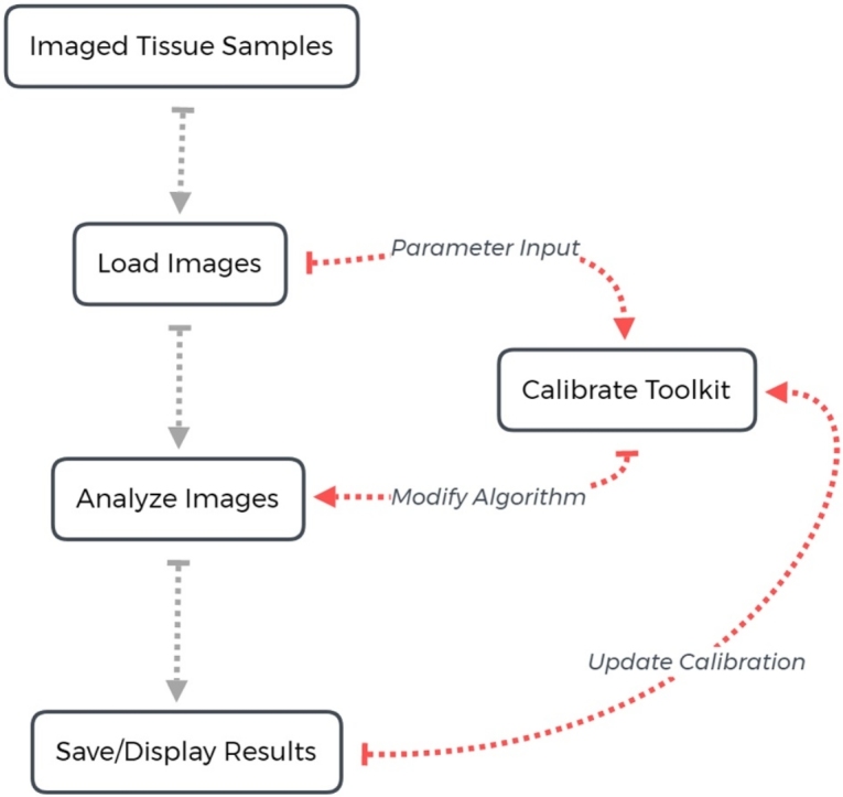
Cardiac structure undergoes a remarkable process of remodeling in response to chronic stress. While the specific structural changes vary across disease states and individuals, a common observation across ischemic and non-ischemic forms of cardiac disease is infiltration and/or activation of non-cardiac cells (e.g. immune cells, fibroblasts) to assist with recovery of the myocardium from injury [[1], [2], [3]]. For example, transaortic constriction (TAC) to induce chronic pressure overload in the mouse induces infiltration of pro-inflammatory monocytes/macrophages, associated with increased fibrosis and cardiac dysfunction [4,5]. Thus, there is interest in the field in describing the remodeling process, often through quantification of tissue properties like fibrosis and infiltration of immune cells – identifiable through immunohistological staining of cardiac tissue sections. However, quantification of these measures may be challenging due to the quantity of data to be analyzed and many groups resort to a qualitative rather than quantitative description. In the interest of improving the rigor, reproducibility and ease of quantifying fibrosis and related phenomena, we describe here a novel suite of open-source, publically available computational tools. Each program is accessible via a user-friendly interface that facilitates calibration and customization to account for variability in image quality. The programs utilize unsupervised machine learning techniques to rapidly and reproducibly quantify the images.

The image analysis suite is comprised of two separate tools: 1) Automated Fibrosis Analysis Tool (AFAT) for quantifying amount of collagen relative to total tissue area in heart tissue sections processed with Masson’s Trichrome staining (collagen stained blue); and 2) Macrophage Analysis Tool (MFAT) for rapid quantification of the number of macrophages in heart tissue sections immunostained with macrophage marker F4/80 [6]. The programs presented here were written in python v3.7, tested with the CPython implementation, and can be run on Windows, OS X or Linux. The algorithms utilize the following libraries obtainable from the Python Package Index (PyPI): numpy, scipy, scikit-learn, scikit-image, PIL, matplotlib, PyQt5, tkinter, xlrd and xlsxwriter. The code can be found on code.osu.edu/hundlab or through hundlab.org/research.

Sample preparation and image acquisition

To fix heart tissue for immunohistochemistry, mice were heparinized, and the hearts were perfused with 10 ml of PBS followed by 20 ml of 4 % paraformaldehyde (PFA)-PBS and then excised and placed in 4 % PFA-PBS for 24 h. Hearts were sectioned and stained using standard methods (Comparative Pathology and Mouse Phenotyping Shared Resource Research Core at Ohio State University) [6,7]. F4/80 antibody (Serotec, catalog number: MCA497 G) was used in immunohistochemistry experiments to identiy monocyte derived macrophages. Images were scanned using an EVOS FL Auto 2 at 40X magnification. They were then stored as tiff files to be read directly by AFAT or MAT. In general, AFAT and MAT are designed to work with numerous different microscope setups, at lower magnifications, and with most common image formats.

Animal studies

Hearts were analyzed from 2-month-old male wildtype and mice expressing truncated β_IV-spectrin [qv^3J, obtained from the Jackson Laboratory [7,8]. WT and qv^3J mice were subjected to transaortic constriction to induce pressure overload conditions, as described [7,9]. Animal studies were conducted in accordance with the Guide for the Care and Use of Laboratory Animals published by the National Institutes of Health (NIH) following protocols that were reviewed and approved by the Institutional Animal Care and Use Committee (IACUC) at The Ohio State University

Overview of the Automated Fibrosis Analysis Tool (AFAT)

AFAT facilitates analysis of Masson’s trichrome stained heart sections for the relative amount of collagen in a repeatable, fast, and accurate manner with an easy-to-operate interface. No programming experience is needed to use the program in its current state. Configuration is possible to adjust for image variability/staining quality, and the code may be easily tailored to suit a different imaging. Briefly, AFAT preforms the following steps to quantify fibrosis as a percentage of the tissue area:

• 1Convert image from RGB to HSV (Hue, Value, Saturation) or CIELAB color spaces, which was defined by the International Commission on Illumination (CIE) to allow for small numerical changes to equate to small differences in perceived color (perceptual uniformity);
• 2Filter image into following groups of pixels: white, red, blue, and pixels that do not readily fit into one of the other groups (undetermined);
• 3Apply linear regression to identify white pixels from undetermined pixels;
• 4Use K-Nearest Neighbors to classify the remaining undetermined points as red, blue, or still undetermined;
• 5Calculate the percent fibrosis as a fraction of blue and red pixels.

AFAT algorithm

The first step for pixel categorization is to use a single pass color filter to classify pixels which are within a preset definition of blue, red or white. The definition was tuned to cover the range of staining saturations and shades typically observed in our sections, but the settings may be re-tuned later to improve the algorithm for different staining protocols. The approach is similar to the algorithm used in ImageJ [10], except that tuning parameters is simpler in AFAT. The color filter by default uses HSV because of its more intuitive definition of color values and saturation. However, RGB values are also made available for use in the color filter when necessary, such as for following the rules used by the ImageJ algorithm. Once classified as white, red or blue, the color label for a pixel does not change in subsequent classification rounds, which focus on pixels that not classifiable by the color filter.

Next, the program classifies white pixels that were left unclassified by the color filter. This is done by building two linear models via regression: one with the known white and red pixels from the previous color filter step, and another using white and blue pixels. The two models are then used to extend the definitions provided in the color filter to classify the white pixels which were skipped by the color filter. To ensure that the pixels are classified correctly, both linear models must agree for a pixel to be classified as white. By using two models instead of one, the bias towards red and blue that are present in each individual model is decreased. Linear models were compared to more complex regression approaches but had similar performance and faster computation time. Computation time at this step is critical, as for images which are not tightly cropped, white pixels will comprise the vast majority of all the pixels present in the image.

In the sample dataset, the average percentage of pixels left unclassified was 0.5 % after linear regression classification. While this is a small section of the whole image, it is on average 2.9 % of the red tissue, which is significant compared to the percentage of fibrosis. Therefore, a more sophisticated algorithm is used (K nearest neighbors) at the next classification step. K nearest neighbors uses a defined number (K) of closest points to the unclassified point to determine its new label. The AFAT algorithm uses the 5 closest neighbors in the CIELAB color-space. The distance between points is measured using the standard Euclidean metric, with the numeric values L*, a*, b* defining a point in 3-dimentional space. CIELAB space was found to be superior to HSV or RGB for this task as colors in CIELAB are designed to be perceptually uniform, which means that a small change in distance equates to a small change in the perceived color, thus making it amenable for use in KNN which relies on accurate distance metrics. Using 5 neighbor points is the standard for the KNN algorithm and changing it did not show a strong impact on the prediction results. In some cases, setting K to another value may be beneficial, however we recommend against setting K to a very large value as that may greatly slow AFAT down. After the 5 closest neighbors are found, their labels (red, blue, white) are used to assign a label for the unknown pixel. A conservative classifier is utilized whereby 4 of the 5 neighbors must agree to the same label for the pixel to be classified. If a pixel fails to meet this requirement, its classification remains undetermined.

Finally, the number of red and blue pixels are calculated and the fibrosis percentage is found as the ratio of blue pixels to the sum of red and blue pixels.

AFAT user interface

AFAT can be launched by double-clicking on the script Automated Fibrosis Analysis Toolkit.py (program will open in python, installation steps are detailed in the associated README file included with source code). Once launched, the program prompts the user for input at three distinct stages. First, the user is asked to select image files to be processed. Multiple files may be selected for batch processing. The second prompt is for the “results file” where the fibrosis percentage and pixel counts will be saved. If this prompt is cancelled, the numerical results will only be displayed onscreen once the analysis is finished. The final prompt asks for a “results directory” where images generated during the analysis will be saved. Again, if no directory is specified, the results will be plotted to the screen.

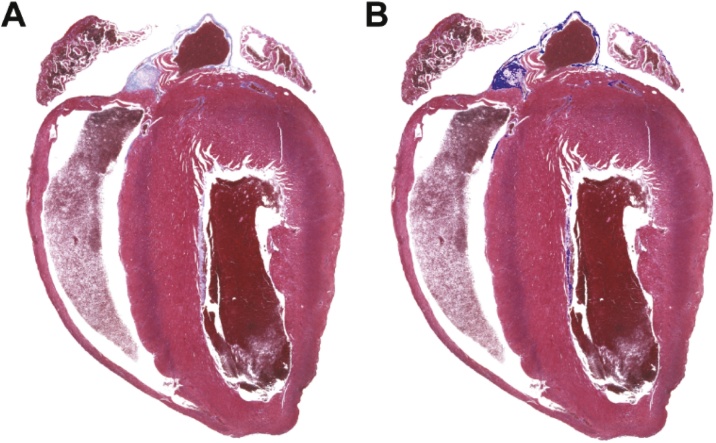
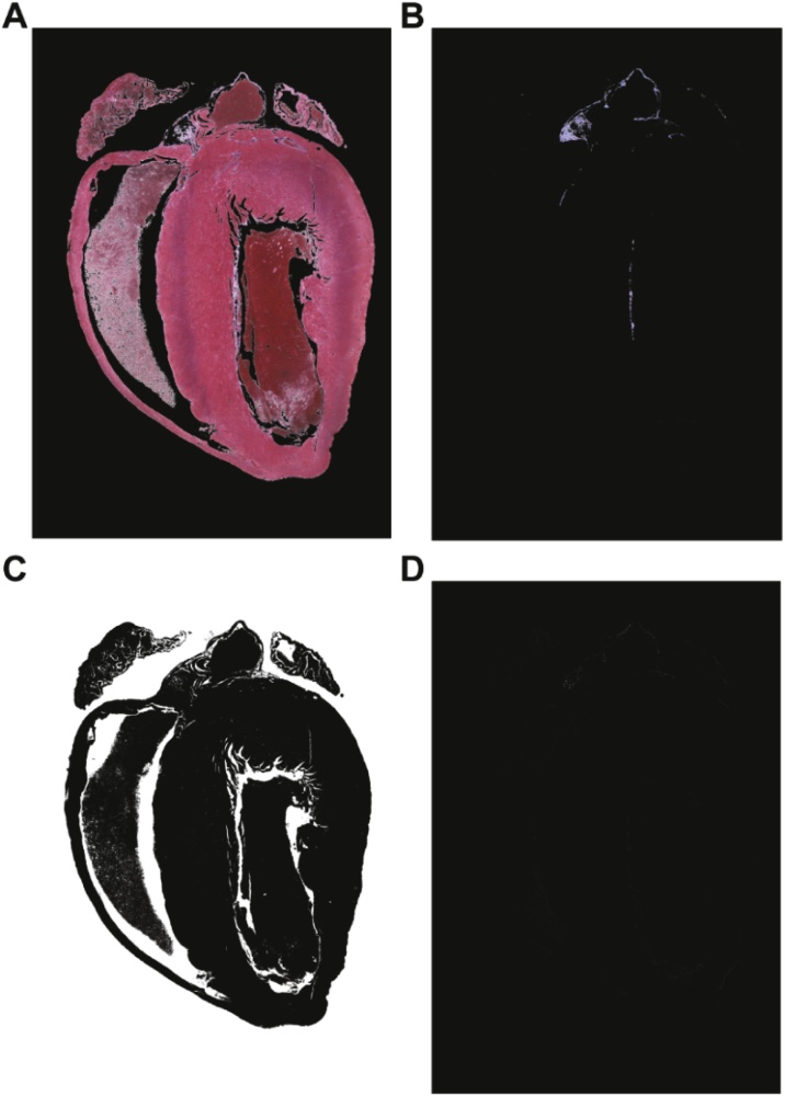
Image processing results are displayed in four plotting windows. The first window displays the original image (Fig. 1A); the second displays the red and blue pixels which were detected (Fig. 2A and B respectively); the third displays white and undetermined (Fig. 2C and D respectively); and the fourth displays the original image with area determined to be fibrosis (blue pixels) highlighted (first and fourth windows shown in Fig. 1). For displaying the red, blue, white and undetermined pixels, everything that is not classified as that color is covered in black so only the relevant portion can be seen (Fig. 2). For visualization of detected fibrosis, blue pixels are highlighted by adjusting the hue in the HSV color-space to be fully saturated, causing them to appear as bright blue.

Fig. 1.

Identification of fibrosis using the automated fibrosis analysis tool (AFAT). Images displayed by AFAT after fibrosis quantification is completed. A) The original Masson’s trichrome stained heart section imported into AFAT. B) Final image with highlighting of regions identified by AFAT as fibrosis (indicated by bright blue).

Fig. 2.

Color classification of pixels in AFAT. (A–D) Color masks indicating pixels identified as red (myocardium), blue (fibrosis), white (background), and unclassified, respectively.

When the analysis is finished, the results, including pixel counts at each stage, are saved in a csv file (“results file” specified by the user) and may be used for subsequent analysis.

Algorithm settings adjustable by user

There are a number of ways to adjust the algorithm without needing to edit large amounts of code. The settings.py script file may be opened in any plain text editor (such as notepad) and contains variables to modify the sensitivity of the algorithms. Most notably, the minimum saturation of blue (min_blue_saturation) can be adjusted to control the lightest shade of blue that will be accepted in the color filter. For the second classification step, there is the n_neighbors value corresponding to K (number of neighbors) in the K nearest neighbors algorithm (default set to 5). Finally, the min_consensus variable adjusts the percentage of neighbors which must agree on a color label before the point can be reclassified as that color (e.g. if this is set to 0 then all undetermined pixels will be classified by their most common neighbor).

Validation of AFAT, comparison to existing analysis tools and limitations

ImageJ is a free and commonly-used application developed by the NIH for low-level processing of digital images and has the capability to analyze the fibrotic content of a histological section using an algorithm developed by the Shapiro lab group [10]. Briefly, the ImageJ program separates the input image into its corresponding red, blue and green layers. Brightness values of the blue layer are then divided by the brightness values of the red layers. Pixels that are 120 % brighter in blue than they are in red are determined to be blue (indicative of fibrosis). Conversely, pixels that are 120 % brighter in red than blue are designated red (indicative of myocardium). The percentage of fibrosis is defined as the ratio of blue pixels to the sum of red and blue pixels. One drawback of this procedure is that images with lower contrast may fail to be appropriately quantified. Additionally, the staining may be highly variable between experiments and adjusting the algorithm to compensate may be difficult. In contrast, AFAT accounts for variability in the resulting blue, by using the KNN to extrapolate from the blue pixels found in the image. The AFAT settings file also allows for much easier and more fine-tuned control, and for adjustments to be made if the staining is substantially different.

Other tools are available that improve on the ImageJ algorithm, but these are largely commercial applications, or for different staining protocols (e.g. picosirius red) [11,12]. Aperio ImageScope’s colocalization is a solution developed by Leica Biosystems (leicabiosystems.com) for use in pathology research and provides useful toolboxes such as their nuclear algorithm which allows quantification of cell nuclei under certain staining conditions. ImageScope uses color deconvolution for quantifying fibrosis in histological sections. Other tools are available for quantification but colocalization is well suited for small batch sizes without the need to use data to train the algorithm.

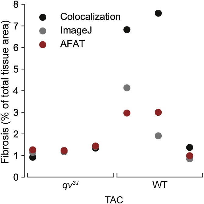
In order to validate AFAT, we compared the results of our fibrosis quantifier to both the ImageJ plugin and the colocalization method in ImageScope on WT and qv^3J mice following 6 weeks of TAC surgery. The qv^3J mice have been shown previously to be resistant to fibrosis and cardiac dysfunction following TAC [7]. All three fibrosis quantifiers yielded similar values for the level of fibrosis in 3 different qv^3J hearts with AFAT producing the lowest standard deviation (Fig. 3). AFAT and ImageJ returned similar values for WT hearts with ImageScope colocalization consistently yielding larger values than the other two programs. While the absolute numbers varied between quantification algorithms, there was agreement across all three platforms that WT hearts showed more fibrosis than qv^3J, consistent with previous reports [7].

Fig. 3.

Comparison of AFAT to existing image analysis programs. Percent fibrosis calculated using AFAT, ImageJ or Aperio ImageScope’s colocalization algorithm, on three independent samples from WT and qv^3J hearts following 6 weeks of trans-aortic constriction (TAC).

Although we have demonstrated that AFAT yields results similar to existing image analysis programs, additional independent validation (e.g. immunoblot for related proteins) would be important going forward to bolster confidence in absolute values returned by the program. It is also important to note that the algorithm is not tuned to differentiate between myocardium and other non-fibrotic tissue components (e.g. blood in the cavity). Thus, pre-processing of the image may be required to remove cavity blood or other elements that might affect calculation of total tissue area by the program.

Overview of the Macrophage Analysis Tool (MAT)

MAT facilitates rapid quantification of macrophage populations using immunostained heart sections. The program takes the image(s) to be processed, guides the user through a simple calibration procedure to ensure data accuracy, and provides enumeration of macrophages including size and location. The output dataset including the calibration information can be saved for reopening as well as exported to an Excel worksheet for further analysis

MAT algorithm

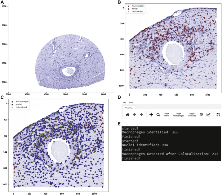
Following preparation and staining procedures, the tissue samples are imaged at 40X magnification and opened in MAT using the procedure detailed below. Due to experimental variability in immunostaining quality and imaging conditions, the detection algorithm must be calibrated for each image set. Upon opening the calibration procedure, as described later, the user is prompted to select cells representative of appropriately stained macrophages. Through an intuitive graphical interface (Fig. 4, discussed in more detail below), the user identifies a center point and radius to define the location of each cell. The RGB tuple for each pixel within these defined borders is normalized by its mean to produce a 3-point color ratio and an independent brightness level. This normalization step serves to mitigate the effects of brightness artifacts left from the imaging procedure. The mean RGB tuple for the entire set is calculated along with a tolerance defined by the range per channel. Finally, a brightness threshold is set at one standard deviation above the average color intensity in order to remove pixels whose color ratio may fall within the tolerance but are too light to be considered a valid match.

Fig. 4.

Main user interface for the macrophage analysis tool (MAT). A) MAT’s main window with an image imported and ready for calibration and processing. B) Preliminary analysis showing cells initially identified as macrophages in red. Analysis can be further improved by generating a nuclear calibration profile and using the colocalization tool found in the Tools menu. C) Completed analysis demonstrating tagged nuclei (blue), macrophages from initial identification (red), and macrophages verified by colocalization (green). D) The File menu has options to open new images and save the identified nuclei macrophages and localized macrophages. The Tools menu has the calibration and processing functions as well as a crop tool. The toolbar includes zoom (magnifier glass) and pan (cross hairs) functionality, as well as toggle buttons for showing/hiding specific markers. E) Representative terminal output from running macrophage detection and colocalization. Results can also be saved using File > Save > Save All CSV Files.

Once the calibration sequence is complete, the user may then run the detection algorithm with the goal of identifying the location of all macrophages (representative identification of macrophages shown in Fig. 4B). In a similar manner to the calibration procedure, the RGB tuple for each pixel in the selected image is normalized by its mean to yield independent metrics of color and brightness. Those pixels that fall within the tolerance range of the calibration tuple and below the brightness threshold are selected as pixels of interest. Gaussian filtering is applied to the selection to smooth noise, followed by a subsequent thresholding step to return the selection to binary values. As the primary directive of this tool is to provide an accurate count of presented macrophages, several steps are taken to ensure proper segmentation of the selected regions of interest. Densely populated regions where two or more cells are adjacent can pose a problem to generating an accurate count if the selected areas for those cells overlap each other. By applying a Gaussian filter, the selected pixels are converted from a binary selection (i.e. either a point of interest or not) into a probability of being a point of interest, with the maximum probability in the center of the region. The threshold following the filtering step is set to eliminate any points that are not greater than 25 % probability. This serves to reduce the edges of the selected regions where borders may intersect.

Next, an erosion operation is performed using a disk-shaped structuring element. This step segments thin regions of high probability along their narrow dimension, further decreasing the likelihood of overlapping regions. The selected regions are then passed into a density-based clustering algorithm (DBSCAN) [13]. This algorithm takes a radius (epsilon) and minimum points value to generate clusters from the input array. If a given point has the minimum value of neighboring points within epsilon, it is determined as a core point and attached to a cluster. If a point is connected to a core point (within epsilon) but does not have the minimum number of adjacent points, it is classified as an edge point and associated with the adjacent cluster of core point(s). Points which do not have the minimum number of neighboring points and are not connected to a core point are assumed to be noise and rejected. The centroid of each cluster is saved as well as the Manhattan distance corresponding to its most distant point. This Manhattan distance serves as a radius measure for the detected cell. The centroids are then plotted on top of the original image within the user interface.

Once macrophages have been detected, a colocalization algorithm is applied to reduce the presence of false positives in the dataset (Fig. 4C). This colocalization algorithm identifies nuclei in the same manner as the macrophages save for using separately gathered calibration data. By using the spatial relationship between potential macrophages and nearest-neighbor nuclei, regions that test positively for the appropriate staining but do not have the required nuclear structure are eliminated. This ability of the program to take advantage of multiple features of the macrophages allows the user to ensure greater precision in their measurements.

MAT user interface

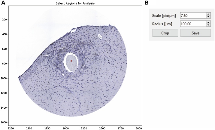
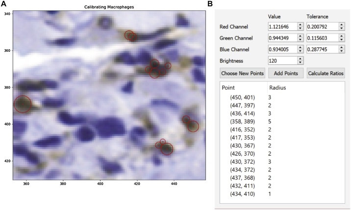
To launch MAT open the script Macrophage Analysis Toolkit.py with python by double-clicking on the script (detailed installation steps are provided in the README file included with source code). First, the user is prompted to select the image for processing, which can be done through the menu bar (File > Open > Open Image) or using the ‘Ctrl + O’ keyboard shortcut (representative image shown in Fig. 4A). If the user would like to limit analysis to perivascular regions, a crop tool can be found under the Tools tab in the menu bar (Fig. 4D). The image selected after choosing the crop tool opens in a new window, after which the user provides the scale factor of the scan [pixels/μm] and the desired radius for consideration. The user is then prompted to select the center of each vascular region by double-clicking and indicated with a red dot (Fig. 5). Selecting crop processes the image and opens it in a new window. Once the selection has been confirmed, the original window can be closed and the save button allows for a directory to be chosen for the cropped image. The image must then be opened in the main window as described above using Open Image. To analyze the image, a calibration profile for both macrophages and nuclei needs to be provided. If this has already been defined and saved in a previous session, the user can reopen the data through the menu bar (File > Open > Open Calibration), and navigate to the appropriate csv file. If the data still needs to be calculated, the calibration menus may be accessed via (Tools > Calibrate). Selection of Choose New Points in the popup menu opens the image in a new window and briefly describes the selection procedure (Fig. 6). The navigation buttons in the toolbar can be used to zoom in on a selection of the image at which point several representative macrophages should be chosen. A double-click defines the center (a red dot will appear on the window) and a right-click will define the radius of the macrophage (a circle will then be drawn with the corresponding radius). Once the desired macrophages are selected, closing the window and pressing the Calculate Ratios button will populate the data boxes with the calculated values (Fig. 6B). If the calculation must be added to or redone, Add Points will reopen the window with the previously-selected macrophages still displayed and Choose New Points will delete the previous selection. For use in later analyses, the calibration may be saved (File > Save > Save Individual CSV > Save Macrophage Calibration). The same procedure is used for defining the nucleus calibration data. Once both sets of calibration data are loaded, processing of the image can be completed by initializing identification of the macrophages (Tools > Process > Macrophages), as seen in Fig. 4B. The python console will update the user on status of calculation (e.g. “started!” followed by a macrophage count and “finished!” when the analysis is complete (Fig. 4E). The nuclei should then be identified in the same manner, before colocalization of the two datasets can be performed.

Fig. 5.

MAT cropping tool. The crop tool can be used to reduce the image to a region or regions of interest. A) The center (red dot) and a desired radius are specified under the “select region for analysis” B) The scale and radius of the crop are specified in a popup box.

Fig. 6.

Generation of a macrophage calibration profile in MAT. A) Using the calibration tool, image sections representative of the cells of interest are selected and an RGB profile for pixel-matching is generated. The centers are chosen by double-clicking and the radius is selected by left-clicking. B) Once representative macrophages are selected for calibration, the “Calculate Ratios” button in the “Calibrating Brown Dots” pop-up menu will create and display calibration values.

Once the analysis of nuclei and macrophages is complete, the user performs the colocalization step to determine those macrophages with nuclei, which increases the accuracy of the analysis by removing staining artifacts. To perform colocalization, select (Tools > Process > Colocalize) and the main window will have the colocalized macrophages marked with a green plus over the original brown macrophage marker (Fig. 4C). The toggle buttons shown in Fig. 4D may then be used to show or hide the nuclei, macrophages, or colocalized macrophages. The locations and radii from each of the analyses may be saved as separate CSV files, or as an excel spreadsheet (File > Save). Calibration data must be imported from CSV files.

Validation of MAT, comparison to existing tools and limitations

Perhaps, the most reliable method for quantification of these data is manual identification by lab personnel. However, this approach is limited by user bias and time demands. Automated methodologies for quantifying macrophage populations (or any cell type) in histological sections are currently limited. ImageJ (discussed above) has a plugin for this application aptly named the color pixel counter allowing for identification of pixels of certain colors (RGBCMY) with a minimum threshold for identification. The data output by this plugin details the number of pixels matching this color range and can be used to quantify an area percentage representative of the specific color. The value of these data are limited however, as a cell count cannot be accurately provided, and the pixels of interest can only be identified if their color matches one of the predefined RGBCMY values. This gives the plugin significant utility when fluorescently-tagged cells are the subject of interest, but makes identification difficult when other tagging/staining methods are used. Aperio ImageScope (commercial suite discussed above) is a commercial option with useful toolboxes such as a nuclear algorithm which allows quantification of cell nuclei under certain staining conditions. This equates to a more complex version of the pixel count provided by ImageJ as the quantification not only provides cell count through the use of clustering algorithms, but is also able to be used with a greater range of identifying markers than the 6 RGBCMY options provided in ImageJ. This means it can be applied to images without fluorescent tags.

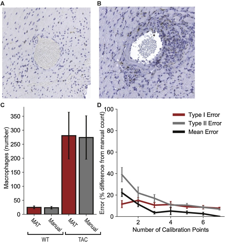
In the interest of generating an accuracy metric for this toolkit, manual quantification was performed by a trained scientist to serve as the true count. A group of 6 images, all from separate wild type (WT) animals was used. 3 mice were subjected to 7 day transaortic constriction (WT TAC) and while the remaining 3 baseline (WT BL) were not. The WT TAC animals demonstrated a markedly higher level of macrophage proliferation than the WT BL allowing for comparison of accuracy across images with different densities (Fig. 7A–C). As the DBSCAN algorithm powering the MAT’s clustering ability is density dependent, it was important to gauge the program’s robustness to such changes in macrophage density. Each image was processed through the toolkit 7 times. The first trial with only one representative macrophage selected and adding another characteristic cell with each successive analysis. The locations of the MAT-identified macrophages for each trial were then compared against those identified in the true count to quantify Type I and Type II error (Fig. 7D). Based on Mean Error curve in the plot shown, it is reasonable to conclude that specifying approximately 4 calibration points is sufficient to provide a count within 5 % of the true value with minimal gains presented by specifying further cells.

Fig. 7.

Validation of MAT through comparison to manual count. Representative images for WT heart sections (A) at baseline and (B) following 7 days of TAC. Nuclei are indicated in blue and macrophages in brown (F4/80 positive). C) Summary data for number of macrophages identified by MAT and by manual counting (N = 3 sections analyzed per group). 4 representative macrophages were used for MAT calibration. D) Estimation of error in analysis as a function of the number of macrophages used for calibration (N = 6 sections analyzed per group). Calibration profiles were derived by selecting between 1 and 7 representative macrophages. Type 1 and type 2 errors were then manually quantified for each trial. Type 1 and Type 2 errors were calculated as percentages of the total number of macrophages, and Mean Error was calculated as the mean percentage difference between MAT and the manual count.

The general applicability of the cell detection algorithm can already be seen in that only recalibration was necessary for it to detect cell nuclei instead of F4/80 stains. This suggests that MAT’s algorithm could also be used to quantify similarly stained features in other images with only recalibration or minor changes. Stained features that MAT would be easily extendable to would have a distinct color with a reasonably continuous shape. As detailed in the methods section of this paper, the calibration process allows a precise definition of the parameters by which identification is made. This results in a paradigm for selection that is not only more versatile than those options afforded by ImageJ and ImageScope, but also more easily repeated than the parameters lab personnel may use for selection.

References

- 1.Yan X. Temporal dynamics of cardiac immune cell accumulation following acute myocardial infarction. J. Mol. Cell. Cardiol. 2013;62(September):24–35. doi: 10.1016/j.yjmcc.2013.04.023. [DOI] [PubMed] [Google Scholar]
- 2.Suetomi T., Miyamoto S., Brown J.H. Inflammation in non-ischemic heart disease: initiation by cardiomyocyte CaMKII and NLRP3 inflammasome signaling. Am. J. Physiol. Heart Circ. Physiol. 2019;317(August):H877–H890. doi: 10.1152/ajpheart.00223.2019. [DOI] [PMC free article] [PubMed] [Google Scholar]
- 3.Prabhu S.D., Frangogiannis N.G. The biological basis for cardiac repair after myocardial infarction: from inflammation to fibrosis. Circ. Res. 2016;119(1):91–112. doi: 10.1161/CIRCRESAHA.116.303577. [DOI] [PMC free article] [PubMed] [Google Scholar]
- 4.Patel B. CCR2+ monocyte-derived infiltrating macrophages are required for adverse cardiac remodeling during pressure overload. JACC Basic Transl. Sci. 2018;3(April (2)):230–244. doi: 10.1016/j.jacbts.2017.12.006. [DOI] [PMC free article] [PubMed] [Google Scholar]
- 5.Bacmeister L. Inflammation and fibrosis in murine models of heart failure. Basic Res. Cardiol. 2019;114(3):19. doi: 10.1007/s00395-019-0722-5. [DOI] [PubMed] [Google Scholar]
- 6.dos Anjos Cassado A. F4/80 as a major macrophage marker: the case of the peritoneum and spleen. Results Probl Cell Differ. 2017;62:161–179. doi: 10.1007/978-3-319-54090-0_7. [DOI] [PubMed] [Google Scholar]
- 7.Unudurthi S.D. βIV-Spectrin regulates STAT3 targeting to tune cardiac response to pressure overload. J. Clin. Invest. 2018;128(December (12)):5561–5572. doi: 10.1172/JCI99245. [DOI] [PMC free article] [PubMed] [Google Scholar]
- 8.Hund T.J. A βIV-spectrin/CaMKII signaling complex is essential for membrane excitability in mice. J. Clin. Invest. 2010;120(10):3508–3519. doi: 10.1172/JCI43621. [DOI] [PMC free article] [PubMed] [Google Scholar]
- 9.Glynn P. Voltage-gated sodium channel phosphorylation at Ser571 regulates late current, arrhythmia, and cardiac function in vivo. Circulation. 2015;132:567–577. doi: 10.1161/CIRCULATIONAHA.114.015218. [DOI] [PMC free article] [PubMed] [Google Scholar]
- 10.Kennedy D.J. Central role for the cardiotonic steroid marinobufagenin in the pathogenesis of experimental uremic cardiomyopathy. Hypertension. 2006;47(3):488–495. doi: 10.1161/01.HYP.0000202594.82271.92. [DOI] [PubMed] [Google Scholar]
- 11.Hadi A.M. Rapid quantification of myocardial fibrosis: a new macro-based automated analysis. Cell. Oncol. 2011;34(August (4)):343–354. doi: 10.1007/s13402-011-0035-7. [DOI] [PMC free article] [PubMed] [Google Scholar]
- 12.Schipke J. Assessment of cardiac fibrosis: a morphometric method comparison for collagen quantification. J. Appl. Physiol. 2017;122(April (4)):1019–1030. doi: 10.1152/japplphysiol.00987.2016. [DOI] [PubMed] [Google Scholar]
- 13.Ester M., Kriegel H.-P., Sander J., Xu X. KDD-96 Proc. 1996. A density-based algorithm for discovering clusters in large spatial databases with noise. [Google Scholar]