Changes in Dipolar Structure of Cardiac Magnetic Field Maps after ST Elevation Myocardial Infarction

Abstract

Background: Pathological changes in cardiac electrophysiology have been investigated in coronary artery disease using magnetocardiography. Aim of this work was to examine the structure of cardiac magnetic field maps (MFM) during ventricular depolarization and repolarization in patients with acute ST elevation myocardial infarction (STEMI).

Methods: Magnetocardiograms were recorded in 39 healthy subjects and 97 patients who had been successfully revascularized after STEMI. Using the Karhunen–Loeve transform, 12 eigenmaps were constructed for six intervals within the QT interval of each subject's signal‐averaged data. The relative information content of the eigenmaps was compared between STEMI patients and healthy subjects.

Results: Relative nondipolar content was between 0.03% and 0.52% higher in the STEMI group, (P < 0.001 for the repolarization intervals). Information content of the first dipolar eigenmap in the STEMI group was reduced by 2.6%–11.7% (P < 0.001 for the repolarization intervals). STT interval was best able to discriminate between groups: area‐under‐the‐curve for nondipolar content was 85.8% (P < 0.001), for the first eigenmap 91.7% (P < 0.001). Severity of infarction was reflected in lower STT interval map 1 content for patients with anterior versus posterior infarction (83%± 11% vs. 87%± 10%, P < 0.05), with wall motion disturbances (84%± 11% vs. 92%± 7%, P < 0.001) and with microvascular obstruction (81%± 12% vs. 87%± 10%, P < 0.05). Regression analysis showed that patients with lower ejection fraction tended to have less information content (P < 0.001).

Conclusion: STEMI is associated with a loss of spatial coherence during repolarization, as quantified by principal component analysis of cardiac MFM.

Ann Noninvasive Electrocardiol 2011;16(4):379–387

Magnetic fields generated by cardiac electrophysiological processes and detectable by superconducting quantum interference devices have been shown to deliver unique information not apparent in the electrical potentials measured at the body surface. ¹ Magnetocardiography (MCG) thus complements electrocardiography (ECG) ² and various approaches have been investigated on how to quantify and visualize characteristics of the cardiac magnetic fields which reflect both physiological processes as well as the corresponding changes induced by cardiac disease. ³ These approaches have focused on the analysis of MCG signals themselves, ⁴ , ⁵ on the examination of magnetic field maps (MFM) which can be derived from multichannel recordings ⁶ , ⁷ and on procedures which localize electrophysiological activity in the cardiac muscle. ⁸ In the context of coronary artery disease (CAD) pathologically induced MCG changes have been reported on the basis of various measures which examine the structure of the MFM. ⁶ , ⁹ , ¹⁰ , ¹¹

An approach that has been applied to examine the overall spatial features of the electrical cardiac cycle is principle component analysis. ¹² Based on orthogonal expansion methods developed by Lux et al., ¹³ it has been possible to reduce the large amount of data information contained in multilead ECG or multichannel MCG measurements and to identify the main spatial patterns contained in body surface potential maps or MFM. Using the principal spatial features identified in the QRST signals on the basis of the Karhunen–Loeve transformation, studies have demonstrated the discrimination of patients at risk for ventricular tachycardia, both in ECG ¹⁴ and MCG ¹⁵ studies. More recently, the QRS, ST, and T wave signals have been examined in patients in the general context of CAD. ¹⁶ , ¹⁷

In most of these and similar studies, the focus has been on the identification of heterogeneity of repolarization as quantified by the signal components believed to reflect the nondipolar content of the spatial patterns. Structured dipolar content is presumed to be contained in the first three eigenvectors with the most information and nondipolar as the amount of information in the eigenvectors beyond the third. ¹⁴ , ¹⁵ In this study, we examined the nondipolar content during various intervals of depolarization and repolarization in patients who had suffered ST elevation myocardial infarction (STEMI) on the basis of multichannel MCG. Furthermore, we also examined the information content in each of the first three eigenvectors which reflect the more structured, dipolar content. The results were compared with those found in age‐matched healthy subjects. We addressed the question whether, in patients who have suffered myocardial infarction, the primary change in the spatial features of the cardiac signals is a shift from the dipolar to the nondipolar or there are also substantial transfers of information within the dipolar components.

METHODS

Subjects

Patients who had been admitted to hospital emergency services in the city of Essen with STEMI and who had been treated interventionally immediately upon admission were eligible for this study. Of 113 patients who received successful invasive diagnosis and revascularization treatment and were stable enough to be transferred to the Department of Biomagnetism in Bochum, MCG was performed in all but 16 patients. Exclusion resulted for the following reasons: arrhythmia (N = 2), artifacts (N = 7), technical problems (N = 4), or nonconsent (N = 3). This left 97 subjects (aged 58.7 ± 11.7 years, 75 male) in the study whose clinical characteristics can be found in Table 1. The normal group consisted of 39 aged‐matched healthy subjects (aged 54.7 ± 9.0 years, 22 male) with no history of cardiovascular disease and normal resting ECG and echocardiograms. The study was approved by the local ethics committee and all subjects gave written informed consent.

Table 1.

Clinical Characteristics of the Study Subjects

	STEMI Patients	Healthy Subjects
Number	97	39
Age (years)	58.7 ± 11.7	54.7 ± 9.0
Gender (m/f)	75/22	22/17
Left ventriculara function (EF in %)a	50.0 ± 10.1
Anterior/inferior myocardial infarction	51/46
1/2/3 vessel disease	58/25/14
RCA/CX/LAD	55/30/65
Wall motion disturbancesa	79
Delayed enhancementa	87
Microvascular obstructiona	43

^aDetermined on the basis of magnetic resonance imaging. CX = circumflex; EF = ejection fraction; LAD = left anterior descending; RCA = right coronary artery.

Data Acquisition

MCG were obtained in all subjects using a 61 channel biomagnetometer (Magnes 1300C, four‐dimensional Neuroimaging, San Diego, CA, USA). The sensor with a diameter of 32.4 cm and a coverage of ca. 825 cm² was placed symmetrically over the upper frontal thorax of the supine subject. Data were recorded at rest for 3 minutes at a sampling rate of 1 kHz with a bandwidth of DC‐200 Hz. To reduce the effects of external noise, data were registered inside a standard 3‐layered magnetically shielded room (AK3b, Vakuumschmelze, Hanau, Germany). In the patients, MCG was performed 5.8 ± 3.0 days after infarction and immediate subsequent successful intervention.

Immediately prior to the MCG acquisition, cardiac magnetic resonance imaging (MRI) was performed using one of two systems: a 1.5 T Twinspeed Excite MRI system (GE Deutschland, Munich, Germany) or a 1.5 T Magnetom Espree (Siemens Deutschland, Erlangen, Germany). Eight channel coils were used and all patients were in the supine position with pulse (GE) or ECG (Siemens) monitoring and gating. Each sequence was obtained during end‐expiratory breath holding. The standard clinical cardiac MRI protocol provides a localizer, cine images of the left ventricle in long and short axes, acquired using a steady‐state free precession (SSFP) sequence with following typical parameters: GE: TE 1.6 ms, TR 3.5 ms, flip angle 45°, slice thickness 8 mm, slice gap 0, phases 20, matrix 224 × 224; Siemens: TE 1.6 ms, TR 50.5 ms, flip angle 80°, slice thickness 8 mm, slice gap 0, phases 25, matrix 256 × 202. After cine images a bolus of gadolinium contrast agent (0.2 mmol/kg bodyweight) (Dotarem, Guerbet or Magnegita, Insight Agents, Heidelberg, Germany) was given i.v. LGE images were acquired 10–15 minutes after contrast injection using an inversion recovery gradient echo sequence (GE: TE 3.1 ms, TR 6.5 ms, TI 180–250 ms, slice thickness 8 mm, slice gap 0, matrix 256 × 192; Siemens: TE 3.4 ms, TR 650–950 ms, TI 250–350 ms, slice thickness 8 mm, slice gap 0, matrix 256 × 174) and the same slice orientation as cine SSFP images.

Data Processing and Analysis

In each subject's MCG data set, overall noise produced by distant artifacts was cancelled using reference channels and low frequency drift was removed by subtracting a fitted stepwise 3rd degree polynomial fit. In the noise reduced data, all cardiac beats were identified on the basis of correlation to a representative QRS template. Beats were then selectively averaged with respect to beat duration in order to avoid the effect of varying heart rates on QT interval. Accordingly, about 65 beats were selected for averaging within ±10 ms of the modal RR interval duration. Using an automated process, ¹⁸ the following times were determined in the signal averaged data: onset and end of the QRS complex as well as onset, apex, and end of the T wave. These times were visually checked and corrected if necessary. The following intervals were extracted for analysis: QT interval, QRS, ST‐segment, T wave, STT interval, and terminal T wave (Tapex‐Tend).

Singular value decomposition was performed on the basis of the Karhunen–Loeve transform (KLT). ¹³ For each subject, the above‐mentioned depolarization and repolarization intervals were examined. For each interval, the input matrix consisted of (61 channels) × (number of samples in the interval). This was used to calculate the covariance matrix and to determine the eigenvalues and eigenvectors. From this, we reconstructed the first 12 eigenmaps based on the coefficients with the highest relative content and ordered them in descending order of the singular values. The relative content of the first three maps with the highest percentage contribution was considered to represent dipolar content. The summed contribution of the remaining maps 3–12 was defined as the nondipolar content. We then compared the percent content of these maps between the normal and STEMI groups for all time intervals. Furthermore, within the STEMI group, percent content was investigated with respect to a number of clinical variables which are associated with the severity of the underlying disease.

The cardiac MR images were analyzed off‐line using commercial software (GE: MASS Analysis plus V 4.0.1, Medis, Leiden, The Netherlands; Siemens: Argus, Siemens, Erlangen, Germany). For assessment of left ventricular function and mass, the end‐diastolic and end‐systolic cine frames were identified for each slice and the endocardial and epicardial borders were manually traced. The end‐diastolic and end‐systolic volumes were then calculated using Simpson's rule (i.e., sum of cavity sizes across all continuous slices). Wall motion abnormalities, the presence of delayed enhancement, and microvascular obstruction were visually assessed and described by using the 16‐segment heart model.

Statistics

Values are generally given as means ± standard deviation (SD). We compared the percent content of the eigenmaps between the normal and STEMI groups for all time intervals on the basis of descriptive statistics and the Mann–Whitney U‐test (two sided). In addition, the capacity of the maps to distinguish between the two groups was examined on the basis of the receiver operation characteristic (ROC) where the area‐under‐the‐curve (AUC) was used as a measure for sensitivity/specificity. In particular, the percent content of the first map (map 1) of the STT interval was compared in sub‐groups of patients based on infarct localization, wall motion disturbances, delayed enhancement, and microvascular obstruction with the Mann–Whitney U‐test, the number of affected vessels was compared with the chi‐square test (both one sided). The relationship to EF was examined on the basis of regression analysis. A P‐value <0.05 was considered statistically significant.

RESULTS

Most of the information content was found in eigenmaps 1–3 in all subjects and in all intervals. Examples which show the first 12 maps of the STT interval for a healthy subject and a STEMI patient with single vessel disease are given in Figure 1. In both subjects, maps 1–3 display a dipolar structure and contain >99% of the information. The remaining maps are increasingly nondipolar and unstructured and, in this example, the content of maps 4–12 of the patient is higher than that of the healthy subject (0.66% vs. 0.11%, respectively). The results for all subjects and intervals revealed that, on average, more than 98% of the content was contained in the first three maps and less than 2% in maps 4–12 (Table 2). However, for the repolarization intervals, the relative content of the dipolar maps was significantly higher in the healthy subjects whereas the nondipolar content was significantly higher in the patient group. The trend was similar for the QT interval and QRS but only statistically significant for the dipolar content of the QT interval.

Figure 1.

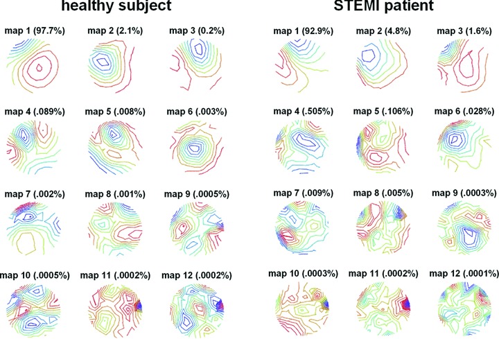
KLT eigenmaps of the STT interval: the first 12 maps of a healthy subject (left) and a STEMI patient (right). The percent information content is given for each map. Maps 1–3 show dipolar spatial features whereas the maps 4–12 are increasingly nondipolar and unstructured. In maps 4–12, the STEMI patient reveals more content.

Table 2.

Percent Content in the Dipolar Maps (1–3) and Nondipolar Maps (4–12) of the Time Intervals for the Healthy Subjects (N = 39) and the STEMI Patients (N = 97). P‐Values < 0.05 in Bold Type

		% Dipolar Content		% Nondipolar Content
		Mean ± SD	P‐Value	Mean ± SD	P‐Value
QT interval	Healthy	98.69 ± 0.65		1.31 ± 0.65
	STEMI	98.11 ± 1.30	0.022	1.83 ± 1.27	0.316
QRS	Healthy	99.05 ± 0.53		0.95 ± 0.53
	STEMI	98.93 ± 0.83	0.092	1.11 ± 0.88	0.810
STT interval	Healthy	99.94 ± 0.05		0.06 ± 0.05
	STEMI	99.62 ± 0.74	0.001	0.39 ± 0.78	0.001
ST segment	Healthy	99.75 ± 0.37		0.20 ± 0.30
	STEMI	99.53 ± 0.49	0.001	0.41 ± 0.43	0.001
T wave	Healthy	99.97 ± 0.02		0.03 ± 0.02
	STEMI	99.88 ± 0.22	0.001	0.13 ± 0.23	0.001
Terminal T wave	Healthy	99.99 ± 0.01		0.01 ± 0.01
	STEMI	99.96 ± 0.06	0.001	0.04 ± 0.06	0.001

STEMI = ST elevation myocardial infarction.

Within the dipolar maps 1–3, most of the information was contained in the first map, some in the second and a minimal amount in the third (Table 3). Generally, the healthy subjects had more content in map 1 than the STEMI patients, whereas they had less content than the patients in maps 2 and 3.These differences were statistically significant only for the repolarization intervals.

Table 3.

Percent Content in the Dipolar Maps 1–3 of the Time Intervals for the Healthy Subjects (N = 39) and the STEMI Patients (N = 97). P‐Values < 0.05 in Bold Type

		Map 1 % Content		Map 2 % Content		Map 3 % Content
		Mean ± SD	P‐Value	Mean ± SD	P‐Value	Mean ± SD	P‐Value
QT interval	Healthy	80.39 ± 9.08		14.50 ± 7.88		3.80 ± 2.23
	STEMI	76.14 ± 11.62	0.097	17.53 ± 9.53	0.096	4.44 ± 2.97	0.324
QRS	Healthy	85.67 ± 9.53		10.39 ± 8.08		2.99 ± 2.21
	STEMI	81.90 ± 11.38	0.239	14.07 ± 10.23	0.066	2.96 ± 2.48	0.696
STT interval	Healthy	96.81 ± 2.90		2.84 ± 2.80		0.29 ± 0.20
	STEMI	85.16 ± 11.01	0.001	12.75 ± 10.02	0.001	1.72 ± 2.09	0.001
ST segment	Healthy	97.83 ± 2.11		1.61 ± 1.60		0.31 ± 0.57
	STEMI	93.75 ± 5.44	0.001	5.13 ± 4.85	0.001	0.65 ± 0.81	0.001
T wave	Healthy	96.47 ± 3.32		3.36 ± 3.29		0.14 ± 0.10
	STEMI	85.77 ± 10.07	0.001	13.37 ± 9.72	0.001	0.73 ± 1.09	0.001
Terminal T wave	Healthy	99.23 ± 0.88		0.73 ± 0.87		0.03 ± 0.06
	STEMI	96.60 ± 4.79	0.001	3.26 ± 4.73	0.001	0.11 ± 0.19	0.001

STEMI = ST elevation myocardial infarction.

ROC analysis of the percent content showed that the repolarization intervals were also able to best discriminate between healthy subjects and STEMI patients (Table 4). Irregardless of the eigenmaps considered, the AUC for the STT interval was consistently the greatest. The best differentiation between subject groups was possible with the information content of the map 1 of the STT interval: AUC was 91.7% and at a cut‐off of 94.8% information content the sensitivity was 87.2%, the specificity 84.5%. Figure 2 demonstrates the results for the repolarization intervals with respect to the nondipolar content and content of map 1.

Table 4.

Area‐under‐the‐Curve (in %) of the Receiver Operation Characteristic (ROC) Analysis for Dipolar and Nondipolar Content of the Different Intervals

	Dipolar Content Map 1–3	Nondipolar Content Map 4–12	Dipolar Content Map 1	Dipolar Content Map 2	Dipolar Content Map 3
QT interval	62.7a	62.7a	60.9a	59.1	55.5
QRS	50.6	50.6	59.2	60.0	47.8
STT interval	86.1a	85.8a	91.7a	89.8a	84.0a
ST segment	70.1a	70.5a	81.3a	81.1a	75.9a
T wave	81.0a	80.6a	89.6a	88.6a	81.9a
Terminal T wave	82.3a	81.9a	77.9a	77.1a	81.3a

^aP < 0.05, P‐values essentially correspond to those in Tables 1 and 2.

Figure 2.

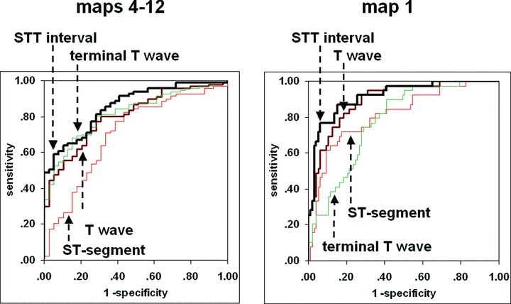
Receiver operation characteristic (ROC) curves for the repolarization intervals with respect to the nondipolar content (maps 4–12) and content of map 1.

As the STT interval was best able to distinguish between healthy subjects and STEMI patients, we also examined the percent content of map 1 of this interval with respect to infarct localization and clinical parameters which are associated with the severity of disease. We found that patients with an anterior infarction had statistically significant less content in STT map 1 than patients with posterior infarction (P = 0.038). Wall motion disturbances, as a measure for the lack of early and effective revascularization, were associated with a greater loss of STT map 1 content (P < 0.001). Furthermore,regression analysis showed that EF had a moderate, positive relationship to STT map 1 content, i.e., lower EF was associated with lower content (r = 0.39, slope = 0.003, P < 0.001). The number of vessels involved did not play a role (P = 0.118). Of the parameters that can be determined on the basis of cardiac MRI, the presence of microvascular obstruction was associated with lower map 1 content (P = 0.012). Although map 1 content was on average lower in patients who displayed delayed enhancement, the differences was not statistically significant (P = 0.122).

DISCUSSION

The main finding in this study is that myocardial infarction leads to a loss of coherent spatial structure in cardiac MFM. This spatial structure was quantified by the information content found in eigenvectors determined using principal component analysis. The loss of coherent structure was evident, on the one hand, in the shift of information content from the maps with a dipolar structure to those with a multipolar structure. It has been proposed that the nondipolarity of cardiac electrical field maps can be characterized by the information content of the KLT eigenvectors beyond the third. ¹⁴ We confirmed this in our examination of MFM for various intervals which comprise the QT interval: the structure of the eigenmaps 1–3 had predominantly dipolar patterns whereas maps 4–12 were generally multipolar. This was true in both the patient group and in the group of healthy subjects. The two groups differed, however, in the fact that the healthy subjects generally had higher information content in the dipolar maps, i.e., the content in the maps of the STEMI patients had shifted slightly but significantly to those with nondipolar structure. This was primarily so for the repolarization intervals in which an up to five‐fold increase of information content was documented.

Examination of nondipolarity in patients after myocardial infarction was first performed in order to assess these patients’ vulnerability to ventricular arrhythmias. ¹⁴ , ¹⁵ , ¹⁹ This is consistent with the results published by Dambrink et al. who showed that nondipolarity may be associated with left ventricular remodeling and altered repolarization characteristics after myocardial infarction. ²⁰ More recently nondipolarity of the T wave in patients with cardiovascular disease has been examined using 12‐lead ECG. ¹⁷ In this and similar studies, T wave residue is defined as the absolute or relative sum of the principal components greater than the third, derived from the singular value decomposition of the signal of the eight independent ECG leads. It has been shown that T wave residue, determined from serial ECGs acquired over ca. 12 hours in patients after onset of STEMI, was on average almost twice as high as that of a control group, indicating that nondipolarity during repolarization is present in the immediate aftermath of myocardial infarction. ²¹ The authors also noted that the dynamics of change of T wave residue values could be associated with the resolution of ST elevation. Furthermore, Schindler et al. have shown that the distribution of Karhunen–Loeve coefficients of the STT segment acquired immediately after presentation in the emergency department can distinguish patients with myocardial infarction (either STEMI or non‐STEMI) from patients without myocardial infarction or patients with unstable angina. ²² In our study, we show that higher nondipolarity can still be detected within days after the acute event and immediate successful revascularization, indicating a shift away from coherent spatial structures to more disorganized patterns.

Apart from the nondipolar content, we also examined the changes in the information content of the individual eigenvectors which make up the dipolar content. It has been suggested that examination of the first three components may be helpful when the relative nondipolar content does not reflect repolarization inhomogeneities accurately. ²³ In our data of both the normal and the patient groups, the relative information content of the nondipolar components was very low (generally <1%): with respect to the total amount of information available in the MFM, the difference in nondipolar content between the two groups was <0.2% on average, and thus minimal. In contrast, when we examined the information content of the individual dipolar maps (maps 1–3), we found substantial differences between the maps of the healthy subjects and those of the patients. Specifically, compared to the healthy subjects, the STEMI patients demonstrated a considerable loss of information in map 1, on average between 3% and 14%, depending on interval. This loss was mainly compensated for by an increase in the content of map 2. The greatest shifts occurred in the repolarization intervals: e.g., in the STT interval 14% and in the T wave 12%. These shifts in information content from the first to the second and, to a lesser degree, the third component are further evidence of a loss of a simple dipolar structure, which in the healthy subjects is dominated by the first eigenmap with up to 99% information content. In the patients, the shift of content consists of a transfer within the dipolar maps and this shift is substantially larger than the increase in nondipolar content.

The individual dipolar maps proved to be more powerful than nondipolar content in the separation between the healthy and patient groups. Taking the loss of content in map 1, ROC analysis showed a higher discriminatory power for all intervals except QT and the terminal T wave when compared to the ROC results based on nondipolar content. The map 1 information loss in the STT interval performed best, with an AUC of 92%. At a cut‐off of 95% content, this gave a sensitivity of 87% and specificity of 84%. In a previous study examining isointegral MCG maps in healthy subjects and patients with ventricular arrhythmias, Hren et al. noted that in the control subjects, the patterns of the QRST maps were primarily determined by the sequence of maps in the STT interval. ¹⁵ In our data, the analysis of the QRS complex resulted in AUC values between 50% and 60% which was not better than chance in identifying patients. Accordingly, the inclusion of depolarization activity in the QT interval also led to relatively poor results. This corroborates the sensitivity of the repolarization intervals. In our results, although the analysis of the T wave on its own performed well, better results in discrimination between healthy and STEMI were achieved when the ST segment and T wave were both included, i.e., in the STT interval.

For the repolarization intervals of the healthy subjects, the first eigenmap contained between 96% and 99% of the total information. In the patients, the information in these first eigenmaps content fell considerably, in the STT interval on average 12%. However, information content varied widely for individual patients: some had content values within in the range of the normals whereas at the other extreme, some patients had content values below 60%, corresponding to a loss of >40%. We postulated that the information loss might be associated with the severity of the infarction and examined a number of clinical measures which reflect compromised cardiovascular function. This could be confirmed for a number of such measures. STEMI patients with poorer left ventricular function, as quantified by EF, tended to greater loss of content in eigenmap 1, as did patients with wall motion disturbances and patients with anterior infarction. Although patients with single vessel disease tended to have somewhat higher relative content, on the whole the number of affected vessels did not correlate clearly to information loss in eigenmap 1. On the other hand, patients in whom microvascular obstruction, as a measure for incomplete revascularization, was present had significantly less content. The presence of delayed enhancement, as a measure for irreversible damage of the myocardium, was also associated with information loss but this could not be statistically confirmed. Taken together, lower information content of the STT interval eigenmap seems to reflect disease severity.

Overall the results suggest that myocardial damage induced by infarction is associated electrophysiological changes which lead to a loss of spatial structure and coherence in MFM, particularly during the repolarization phase. These changes can be adequately quantified on the basis the loss of information content of the first eigenvector map of STT interval activity. This measure may be useful in patients who have suffered myocardial infarction in assessing success of treatment in the acute phase immediately following the event as well as the myocardial recovery in the follow‐up period. Considering that inhomogeneity of repolarization is reflected in STT eigenmap information, the latter may also serve as a predictor of dysrhythmogenic conditions. The study of patient data after appropriate follow‐up times may reveal the capability to identify patients with vulnerability to ventricular arrhythmias or those with deteriorating left ventricular function. Furthermore, it might be of interest to examine dipolar content of repolarization in the broader context of CAD, i.e., in patients who have not had myocardial infarction but in whom ischemia due to stenosis of the coronary arteries is present.

Overall, the results indicate not only that the nondipolar content of MFM in patients with acute symptoms of CAD increases but also that the coherence in the dipolar maps is compromised, particularly during repolarization. Principal component analysis of cardiac MFM using the KLT may thus be helpful in the surveillance of patients with CAD.

Limitations

It should be noted that the time period between the acute event and the MCG measurement varied from a few days to over a week. From ECG, it is known that repolarization processes may change substantially in the days following MI. Thus, the changes in eigenmap content may have been influenced accordingly and led to increased variability in the results. Furthermore, patients with extensive damage remained on intensive care for longer periods and were not eligible for transport to the MCG facilities. This resulted in a selection of subjects with a preference for patients who were in a more stable condition. This is apparent the relatively high EF values in the patient group. The loss of spatial coherence in the patients we could not examine may be expected to be greater than what we have reported here.

REFERENCES

- 1. Koch H. SQUID magnetocardiography: Status and perspectives. IEEE Trans Appl Superconduct 2001;11:49–59. [Google Scholar]
- 2. Lant J, Stroink G, ten Voorde B, et al Complementary nature of electrocardiographic and magnetocardiographic data inpatients with ischemic heart disease. J Electrocardiol 1990;23:315–322. [DOI] [PubMed] [Google Scholar]
- 3. Stroink G, Hailer B, Van Leeuwen P. Cardiomagnetism In Andrä W, Nowak H. (eds.): Magnetism in Medicine. Weinheim , Wiley‐VCH, 2006, pp. 164–209. [Google Scholar]
- 4. Hänninen H, Takala P, Mäkijärvi M, et al Recording locations in multichannel magnetocardiography and body surface potential mapping sensitive for regional exercise‐induced myocardial ischemia. Basic Res Cardiol 2001;96:405–414. [DOI] [PubMed] [Google Scholar]
- 5. Hailer B, Van Leeuwen P, Lange S, et al Spatial dispersion of the magnetocardiographically determined QT intervals and its components in the identification of patients at risk for arrhythmia after myocardial infarction. Ann Noninvasive Electrocardiol 1998;3:311–318. [Google Scholar]
- 6. Van Leeuwen P, Hailer B, Lange S, et al Quantification of cardiac magnetic field orientation during ventricular de‐ and repolarization. Phys Med Biol 2008;53:2291–2301. [DOI] [PubMed] [Google Scholar]
- 7. Jurkko R, Mäntynen V, Tapanainen JM, et al Non‐invasive detection of conduction pathways to left atrium using magnetocardiography: Validation by intra‐cardiac electroanatomic mapping. Europace 2008;11:169–77. [DOI] [PubMed] [Google Scholar]
- 8. Moshage W, Achenbach S, Gohl K, et al Evaluation of the non‐invasive localization accuracy of cardiac arrhythmias attainable by multichannel magnetocardiography (MCG). Int J Card Imaging 1996;12:47–59. [DOI] [PubMed] [Google Scholar]
- 9. Hänninen H, Takala P, Makijarvi M, et al Detection of exercise‐induced myocardial ischemia by multichannel magnetocardiography in single vessel coronary artery disease. Ann Noninvasive Electrocardiol 2000;5:147–157. [Google Scholar]
- 10. Lim HK, Kwon H, Chung N, et al Usefulness of magnetocardiogram to detect unstable angina pectoris and non‐ST elevation myocardial infarction. Am J Cardiol 2009;103:448–454. [DOI] [PubMed] [Google Scholar]
- 11. Ogata K, Kandori A, Watanabe Y, et al Repolarization spatial‐time current abnormalities in patients with coronary heart disease. Pacing Clin Electrophysiol 2009;32:516–624. [DOI] [PubMed] [Google Scholar]
- 12. Castells F, Laguna P, Sörnmo L, et al Principal component analysis in ECG signal processing. EURASIP J Adv Sig Pr 2007;2007:1–21. [Google Scholar]
- 13. Lux RL, Evans AK, Burgess MJ, et al Redundancy reduction for improved display and analysis of body surface potential maps, I: Spatial compression. Circ Res 1981;49:186–196. [DOI] [PubMed] [Google Scholar]
- 14. Hubley‐Kozey CL, Mitchell LB, Gardner MJ, et al Spatial features in body‐surface potential maps can identify patients with a history of sustained ventricular tachycardia. Circulation 1995;92:1825–1838. [DOI] [PubMed] [Google Scholar]
- 15. Hren R, Steinhoff U, Gessner C, et al Value of magnetocardiographic QRST integral maps in the identification of patients at risk of ventricular arrhythmias. Pacing Clin Electrophysiol 1999;22:1292–1304. [DOI] [PubMed] [Google Scholar]
- 16. Garcia J, Wagner G, Sornmo L, et al Temporal evolution of traditional versus transformed ECG‐based indexes in patients with induced myocardial ischemia. J Electrocardiol 2000;33:37–47. [DOI] [PubMed] [Google Scholar]
- 17. Zabel M, Malik M, Hnatkova K, et al Analysis of T‐wave morphology from the 12‐lead electrocardiogram for prediction of long‐term Prognosis in male US veterans. Circulation 2002;105:1066–1070. [DOI] [PubMed] [Google Scholar]
- 18. Van Leeuwen P, Geue D, Poplutz C, et al Reliability of automated determination of QRST times in ECG and MCG. Biomed Tech 2003;48(suppl 1):370–371. [Google Scholar]
- 19. Stellbrink C, Mischke K, Stegemann E, et al Spatial features in body surface potential maps of patients with ventricular tachyarrhythmias with or without coronary artery disease. Int J Cardiol 1999;70:109–118. [DOI] [PubMed] [Google Scholar]
- 20. Dambrink JH, SippensGroenewegen A, van Gilst WH, et al Association of left ventricular remodeling and nonuniform electrical recovery expressed by nondipolar QRST integral map patterns in survivors of a first anterior myocardial infarction. Captopril and Thrombolysis Study Investigators. Circulation 1995;92:300–310. [DOI] [PubMed] [Google Scholar]
- 21. Kesek M, Bjorklund E, Jernberg T, et al Non‐dipolar content of the T‐wave as a measure of repolarization inhomogeneity in ST‐elevation myocardial infarction. Clin Physiol Funct Imaging 2006;26:362–370. [DOI] [PubMed] [Google Scholar]
- 22. Schindler DM, Lux RL, Shusterman V, et al Karhunen–Loève representation distinguishes ST‐T wave morphology differences in emergency department chest pain patients with non‐ST‐elevation myocardial infarction versus nonacute coronary syndrome. J Electrocardiol 2007;40(6 Suppl):S145–S149. [DOI] [PMC free article] [PubMed] [Google Scholar]
- 23. Biagetti MO, Arini PD, Valverde ER, et al Role of dipolar and nondipolar components of the T wave in determining the T wave residuum in an isolated rabbit heart model. J Cardiovasc Electrophysiol 2004;15:356–363. [DOI] [PubMed] [Google Scholar]