Automated QT Analysis That Learns from Cardiologist Annotations

Abstract

Background: Reliable, automated QT analysis would allow the use of all the ECG data recorded during continuous Holter monitoring, rather than just intermittent 10‐second ECGs.

Methods: BioQT is an automated ECG analysis system based on a Hidden Markov Model, which is trained to segment ECG signals using a database of thousands of annotated waveforms. Each sample of the ECG signal is encoded by its wavelet transform coefficients. BioQT also produces a confidence measure which can be used to identify unreliable segmentations. The automatic generation of templates based on shape descriptors allows an entire 24 hours of QT data to be rapidly reviewed by a human expert, after which the template annotations can automatically be applied to all beats in the recording.

Results: The BioQT software has been used to show that drug‐related perturbation of the T wave is greater in subjects receiving sotalol than in those receiving moxifloxacin. Chronological dissociation of T‐wave morphology changes from the QT prolonging effect of the drug was observed with sotalol. In a definitive QT study, the percentage increase of standard deviation of QT_c for the standard manual method with respect to that obtained with BioQT analysis was shown to be 44% and 30% for the placebo and moxifloxacin treatments, respectively.

Conclusions: BioQT provides fully automated analysis, with confidence values for self‐checking, on very large data sets such as Holter recordings. Automatic templating and expert reannotation of a small number of templates lead to a reduction in the sample size requirements for definitive QT studies.

The electrocardiographic QT interval is a clinically important measurement because, when abnormal, it is a harbinger of both cardiac and arrhythmic deaths. ¹ In addition, most regulatory agencies, in accordance with the International Conference on Harmonisation, require an assessment of the effects of new drugs upon the QT interval for their approval and appropriate labeling. ² There are three persuasive reasons for automation of the measurement of QT. First, the measurement can only be made accurately by an expert, and the required expertise is relatively rare: that of a certified cardiologist with special training in and awareness of the practice and pitfalls of QT measurement. Second, the volume of ECGs that must be recorded properly to assess a drug's cardiac repolarization effects is enormous, often exceeding 100,000 12‐lead tracings during the premarketing assessment of a new drug. Accurate automated annotation of the QT could greatly reduce the expense of measurements made by expert readers. Currently regulatory agencies do not consider existing commercial QT measurement algorithms to be acceptably accurate. ² Third, a reliable QT measurement automation technology would allow the use of all the ECG data recorded during continuous Holter monitoring, rather than intermittent 10‐second ECGs, and this would greatly enhance the assessment of cardiac repolarization.

Current automated methods for QT interval measurements typically rely on identifying the end of the T wave as the intersection between a tangent to the waveform and the isoelectric line. ³ , ⁴ These methods have proved not to be particularly robust in the presence of unusual waveform morphologies (e.g., inverted/biphasic T waves or ectopic beats) and noisy signals (60 Hz interference, muscle artifact, baseline wander). More importantly, automated techniques usually provide no associated confidence measures which could identify those beats that the system cannot, and should not, analyze, either because of noise, artifact or abnormal waveform morphology. This lack of self‐assessment has contributed to a reluctance by the pharmaceutical industry and regulatory authorities to adopt the use of automated algorithms for QT analysis.

In this article, we introduce BioQT, an automated QT analysis system based on a model trained on thousands of examples. BioQT reports both the QT interval for that beat and a confidence value associated with that measurement. In addition, BioQT automatically generates templates of beat families according to T‐wave shape. These templates may be reannotated by an expert cardiologist, after which the annotations can be applied to all the beats in the recording.

METHODS

Hidden Markov Models

BioQT is an automated ECG interval measurement technique based on probabilistic dynamic signal segmentation. The dynamic model, a Hidden Markov Model (HMM), is trained to segment ECG signals using a database of thousands of ECG waveforms previously annotated by expert cardiologists.

Figure 1 shows a typical HMM for ECG segmentation. The model architecture is composed of a “hidden” state sequence (indicated by the clear nodes), which is stochastically related to the observed ECG signal (indicated by the shaded nodes). This model is composed of five unique states, which represent, in this instance, the sections of ECG from P to Q, from Q to R, from R to S, from J to T and finally the section from the end of the T wave to the start of the P wave of the following heart beat (“Baseline or B”). This is only one of a possible set of HMM architectures; others are discussed in reference 5 and some of the results presented in the next section were obtained with a different model known as the Q–R–J–T model.

Figure 1.

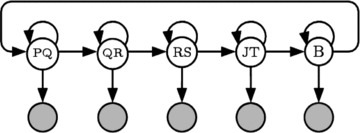
A Hidden Markov Model with five states for ECG segmentation.

At the heart of HMMs are two probabilistic functions, one of which quantifies the probability of the state of interest at a particular time step given the value of the state at the previous time step, and another which quantifies the probability of observing a particular signal value given knowledge of the state. These two probabilistic functions can be evaluated on a sample‐by‐sample basis over the entire course of an ECG waveform and then used to segment the waveform into its P, Q, R, S, and T components. In addition, the probabilistic nature of the HMM makes it possible for a confidence measure to be computed to quantify the validity of the segmentation (see below).

Wavelet Representation of ECG Signal

For ECG segmentation, the hidden state corresponds to a particular waveform feature (i.e., one of PQ, QR, RS, JT, or baseline) which is active at time t, and the observed signal sample corresponds to the associated ECG sample representation at that time. Although it is possible to use the raw ECG signal samples as the input to the HMM, we have found that in practice the accuracy of the model segmentations can be improved considerably by incorporating “contextual information” from neighboring signal samples into the ECG representation. For this purpose, we use a sample‐wise encoding of the ECG derived from a wavelet transform of the signal. ⁵

Wavelets are a class of functions that are well localized in both the time and frequency domains. They are able to capture the nonstationary spectral characteristics of a signal by decomposing it over a set of atoms which are localized in both time and frequency. These atoms are generated by scaling and translating a single mother wavelet. The result of a wavelet transform of a signal is a set of coefficients which capture the activity of the signal over a range of different frequencies (or “scales”) and at a number of different time points.

BioQT makes use of a particular class of wavelet transform known as the “undecimated wavelet transform” or (UWT). ⁶ The UWT is particularly well suited to ECG interval analysis as it provides a time–frequency description of the ECG signal on a sample‐by‐sample basis. In addition, the UWT coefficients are translation‐invariant (unlike, e.g., the coefficients of the discrete wavelet transform), an ideal property for waveform segmentation. Thus each successive sample of the ECG signal (the observations in the HMM) is encoded by its UWT coefficients in BioQT, as shown in Figure 2 for an eight‐coefficient model for one ECG cycle.

Figure 2.

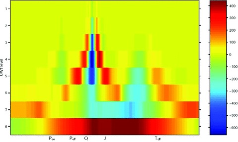
Undecimated wavelet transform (UWT) of ECG waveform—sample number on horizontal axis (500 samples/s), wavelet scale on vertical axis and intensity in color.

The computational overhead associated with computing the wavelet transform is an insignificant fraction of the overall computational time. UWT computation can be implemented efficiently using a filter‐bank structure. BioQT processes a 24‐hour Holter recording in 3–4 minutes on a Dell 390 workstation, with the UWT computation taking a few seconds in total.

The wavelet representation of the ECG offers a number of advantages over the use of the raw ECG signal as the input to the HMM. First, each UWT “observation vector” encodes information about the ECG waveform morphology evaluated over a local window at each time point. This provides the HMM with a form of context, which enables the model to perform the ECG waveform segmentation more accurately. In addition, the UWT coefficients encode the spectral content of the ECG signal (on a sample‐by‐sample basis) over the entire range of frequencies. Hence any low‐ or high‐frequency noise (such as baseline wander or 60 Hz interference, respectively) is captured in different elements of the wavelet feature vector. Since this information is included in the ECG representation, BioQT is able to produce confidence measures (see below) which allow it to differentiate between clean ECG signals and noisy or corrupted signals (for which QT measurements should not be made).

Training the Hidden Markov Model in BioQT

A HMM is parameterized by the following three sets of parameters: (a) the initial state distribution; (b) the state transition matrix A_ij; and (c) the set of observation probability models B_k for each state k (in our case the probability distribution of the UWT coefficients for state k). The training procedure for the HMM is described below.

The data set used to train the BioQT HMM was assembled from the placebo arm of a thorough phase 1 QT/QT_c study. This data set contains approximately 20,000 10‐second 12‐lead ECGs which were recorded (at a sampling rate of 500 Hz) from 380 healthy normal volunteers. For each 10‐second ECG, three consecutive beats were annotated by the expert cardiologists, who identified the following points within each beat and marked them on the digitized waveform with electronic callipers:

• • P‐wave onset (P_onset)
• • QRS onset (Q_onset)
• • R peak (R_peak)
• • QRS offset (J)
• • T‐wave offset (T_offset)

The annotations provided by the experts allow the transitions from one state to the next to be identified and so each sample within the ECG waveform can be given the appropriate state label (i.e., the value of k for that sample). The initial state distribution and the elements of the transition matrix A_ij are computed from the interval durations derived from the expert annotations using maximum likelihood estimates. ⁵ The observation probability densities B_k for each state k are obtained by fitting a Gaussian Mixture Model (GMM) to the wavelet coefficient data for the time samples that occur during the interval corresponding to the given state, for the set of ECG waveforms in the training set. The parameters of the GMM are learnt using the expectation‐maximization algorithm. ⁵

Once the parameters of the model have been learnt, for each lead, BioQT can be used to segment new ECG waveforms. The most probable state sequence S* for a given ECG waveform is inferred through the use of the Viterbi algorithm. ⁷ This state sequence indicates the samples at which the state transitions occur, and hence provides a computer‐derived set of P_onset, Q_onset, R_peak, J, and T_offset annotations.

Confidence Measure for Automated QT Interval Measurements

A key advantage of a probabilistic model such as BioQT over traditional methods of automated ECG segmentation is the ability of such a model to produce a confidence measure for each ECG waveform analyzed. The confidence measure is generated by evaluating the natural logarithm of the likelihood of the observed waveform and the optimal hidden state sequence over the course of the segmented waveform. This log likelihood is then transformed to produce a confidence value between 0 and 1. ⁸ The confidence measure in effect quantifies the “closeness” of the waveform under consideration to the 20,000 exemplar waveforms stored in the training database. There should be more confidence in the segmentation of ECG waveforms similar to those used for training the model than in the segmentation of waveforms which are very different from those in the training data set. The confidence measure can therefore be used to identify segmentations (and hence QT interval measurements) which are unreliable, due to either unusual waveform morphologies (e.g., flat T waves or ectopic beats) or noisy signals (60 Hz or muscle artifact).

BioQT can be used to analyze both conventional 10‐second ECGs or 24‐hour 12‐lead Holter recordings. With the latter, the Q–R–J–T model is often used for QT interval measurement, rather than the full five‐state HMM. The Q–R–J–T model only outputs annotations for the Q_onset, R_peak, J, and T_offset points. It uses two separate HMMs, which only process subsegments of the ECG waveform, the first to detect the Q_onset and J points and the second to detect the T_offset point. Confidence values for the Q–R–J–T model are based on the window of data processed by the HMM that locates the T_offset point. Any waveform whose confidence falls below a given threshold (usually set at 0.7) is then set aside (see later).

Once a 24‐hour Holter tape has been analyzed, BioQT produces a time‐series of QT interval measurements using the Q–R–J–T HMM. Such measurements will inevitably be noisy to an extent, due mostly to artifacts and noise present in the ECG signal. We exploit the fact that each QT measurement is part of a time‐series, representing a quantity expected to change relatively slowly over time, to smooth out some of the noise in these measurements. We therefore use a simple 10‐point moving average, each QT interval measurement being taken as the average of a 10‐beat window of beats. In the case where the measurement is missing for a particular beat (when the confidence value is below the rejection threshold of 0.7), the QT value for that beat is taken to be the same as for the previous beat.

Heart Rate Correction

The standard heart rate corrections (Bazett and Fridericia) can be applied to the QT interval measurements derived by the BioQT software, but we have also investigated heart rate corrections based on the time variation of the QT/RR relationship for that subject. For example, an individual contemporaneous correction, QT_cIc, can be calculated from the regression of the QT interval against the RR interval on the day of treatment, for a given subject, using the following formula:

where Δ(QT/RR) is the gradient of the observed QT–RR linear regression over the time period of interest and the QT and RR intervals are expressed in milliseconds. We have applied this correction formula for sliding windows of different durations (6 and 4 hours) to provide heart rate correction formulae which are localized in time. In each case, the sliding window is centered on the beat to be corrected.

T‐Wave Shape Descriptors

It is now accepted that drug‐induced changes in ventricular repolarization can lead not only to prolongation of the QT interval but also to changes in the shape of the T wave.

Shape descriptors are therefore used to characterize the JT segment of the ECG using frequency‐domain analysis, by constructing what is known as the analytic signal. For shape characterization purposes, it is the ECG waveform itself which is considered rather than the UWT coefficients. The JT segment is firstly smoothed using principal component analysis (PCA), whereby only the first few principal components in a singular‐value decomposition of a set of consecutive JT waveforms are retained and used to reconstruct a set of smoothed waveforms.

Each smoothed JT segment is then decomposed into a series of sine and cosine waveforms whose frequencies are integer multiples of the fundamental frequency. From the amplitude and phase signals, the following shape features s_n are computed:

• • sine of the initial value of the phase signal;
• • cosine of the initial value of the phase signal;
• • initial gradient of the phase signal;
• • final gradient of the phase signal;
• • difference between the phase signal at the start and end; and
• • maximum value of the amplitude signal.

These features s₁ to s₆ are concatenated into a six dimensional shape vector {s₁, …, s₆} which describes the shape of the corresponding JT segment. Several of the features of the shape vector have been observed to be correlated with heart rate, and so those morphology differences are tracked by the shape vector.

The novelty of the shape of a JT segment can be assessed with respect to the BioQT model of normal T‐wave shapes. This is a set of 500 prototypical six dimensional shape descriptors, which were extracted from the original data set of 20,000 ECG waveforms using a standard clustering algorithm (k‐means clustering). The probability density function for these 500 shape vectors, representative of normal shapes, is computed using a Parzen Windows density estimator. ⁹

Once the parameters of this density estimator (number of cluster centers and their width) have been set, the estimator can be used to compute the likelihood P that the shape of any JT segment is normal. With BioQT, the “morphology novelty indicator” is the associated log likelihood. The more novel the shape of a T wave in a JT segment is, the smaller the value of P and hence the more negative the log likelihood will be.

Automated Generation of Templates Using Shape Descriptors

The BioQT software also uses the shape descriptors for the automatic generation of templates, to try and identify beats with unusual waveforms. The latter arise either because the waveform is corrupted by noise or artifact, or because the study drug causes changes in the morphology of the T wave. It is very important to identify the latter, and BioQT automatically generates templates which characterize groups of beats with unexpected T‐wave shapes, that is, “novel beats.” These can then be reviewed by an expert cardiologist, who will be able to distinguish between noisy or artifactual beats and those novel beats with unusual T‐wave morphology. Although there are around 100,000 beats to analyze for each lead in a 24‐hour Holter study, the BioQT software only produces between 10 and 20 templates for the cardiologist to review, that is, the number of waveforms requiring expert review is reduced up to 10,000‐fold. The cardiologist can also choose to reannotate the template, if the unusual morphology has caused the T_offset estimate to be inaccurate, and all the beats characterized by that template are then automatically reannotated by the BioQT software, as explained below.

The shape vectors are used in an on‐line “templating algorithm” which assembles templates of the different T‐wave morphologies in the ECG recording. The shape of the T wave is assumed to be normal at the start of the drug study and so the initial template is the average six dimensional shape descriptor from, say, the first 15 minutes of the recording period. The six dimensional shape descriptor for each subsequent JT segment is tested against this initial template. When the Euclidean distance between the shape descriptor and the template is greater than a given threshold, a new template is created: this template is the average waveform for the family of beats which has this novel T‐wave morphology. The shape of subsequent JT segments is now tested against both the initial template and the new template; again, when the Euclidean distance between a six dimensional shape descriptor and its closest template (in six dimensional space) is greater than the threshold, a new template is created. This process continues until the entire 24 hours of ECG data have been analyzed. The value of the threshold chosen controls the number of templates generated and experience acquired over a number of QT studies has enabled us to set this threshold so that the number of templates generated remains below 20.

Refined Analysis

All of the analysis described above is fully automated: for every beat, the BioQT software produces a QT interval estimate, together with a confidence value associated with that estimate, and a scalar parameter indicating the novelty of the T‐wave shape with respect to the normal ECG waveforms stored in the training data set. Templates which characterize the different shapes of the T wave encountered during the course of the drug study are also generated automatically.

A completely automated report, based on high‐confidence beats only, can therefore be generated at this stage but BioQT goes an additional stage by producing a refined analysis using an additional software tool for the expert cardiologist. This tool (described more fully in the Results section) allows the cardiologist to review the templates generated by the BioQT software, and either reannotate them or reject them as noise or artifact. As explained above, the BioQT software only produces between 10 and 20 templates for the cardiologist to review, and so the number of waveforms requiring expert review is highly manageable.

If a template has been generated by a family of novel beats with unusual morphology, the estimate of T_offset produced by BioQT may be inaccurate and the refined analysis tool allows the cardiologist to reannotate the template. This reannotation is then applied automatically to all the beats in the recording with a similar T‐wave shape. These are the beats for which the JT segment shape descriptor is closest in six dimensional Euclidean space to the template shape descriptor. The beats belonging to this family of beats will, of course, all have different durations, depending on the heart rate at the time. To cope with this variability, the reannotations of the template beat are reapplied to every beat in the family using Dynamic Time Warping (DTW). The use of DTW is common in automated speech recognition: ¹⁰ it allows the various sounds in a word to be stretched and compressed by different amounts when trying to match an unknown utterance against a number of templates, each of which corresponds to a different word. Here DTW is the process of matching each ECG waveform in the family of beats to the template waveform by local nonlinear stretching and compression of the time axis. As the heart rate varies, a simple linear rescaling of the time axis tends to result in the different features (e.g., the R_peak and T_peak) being located at a spread of different positions. The DTW software in BioQT maps the template annotations to each beat in a family, all of which have a similar shape but different durations.

The on‐line templating algorithm in BioQT has been used to highlight beat families in 24‐hour Holter recordings that require reannotation by a cardiologist. This strategy allows for an entire 24 hours of QT data to be reviewed by a human expert and for the template annotations to be applied to all beats in the recording, all in a few minutes. In addition, the algorithm provides a mathematically principled but visually simple means of tracking T‐wave morphology and hence of identifying novel T‐wave shapes.

RESULTS

BioQT has now been applied to a number of ECG data sets on which it has out‐performed conventional QT measurements methods. Figures 3 and 4 show the QT interval segmentations (i.e., from Q_onset to T_offset) calculated by the automated BioQT system, together with the respective confidence values, for two sets of ECG waveforms: first, a high‐quality set of waveforms (Fig. 3) for which the confidence values are around 0.94 and second a set of more noisy waveforms (Fig. 4), for which the confidence values are lower, but still acceptable; two out of three waveforms have a confidence value just above 0.7.

Figure 3.

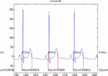
Three high‐quality ECG waveforms and the corresponding QT interval measurements calculated by the automated BioQT system, together with the associated confidence values (on a scale of 0–1), which are all close to 0.94.

Figure 4.

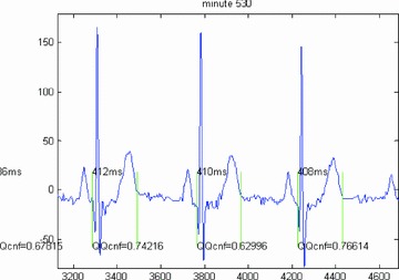
Three noisy ECG waveforms and the corresponding QT interval measurements calculated by the BioQT system, together with the associated confidence values (on a scale of 0–1), which vary between 0.63 and 0.77.

BioQT's performance on a set of ECG waveforms containing an ectopic beat is shown in Figure 5. Note also that this ECG signal has an inverted QRS complex. The ectopic beat affects the two central ECG waveforms (beats 2 and 3). The QT intervals for beats 1 and 4, which are normal, are 398 and 404 ms, respectively and both have a confidence value of 0.86. The QT interval for beat 2, however, is 644 ms, but it has a confidence value of 0.00, and that for beat 3 is 472 ms, with a confidence value of 0.04. The use of confidence values allows BioQT to detect automatically unreliable interval measurements.

Figure 5.

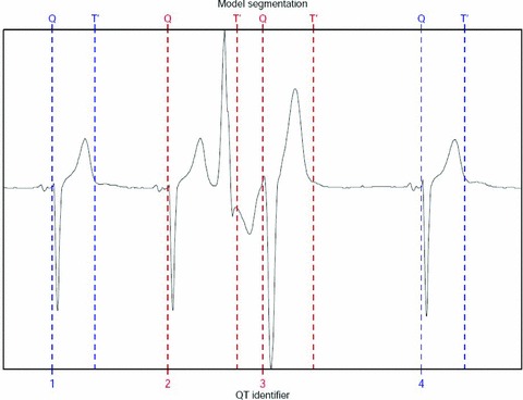
Four consecutive ECG waveforms with an ectopic beat (beat 2) and subsequent distorted beat (beat 3). Beats 1 and 4 are normal ECG waveforms.

The BioQT software has also been used to analyze the sotalol data previously presented by Sarapa et al. ¹¹ In this study, the mean change in QT interval was analyzed for a number of healthy volunteers given two different doses of sotalol:

• Day 1: 

  Baseline—39 patients

• Day 1: 

  Single dose of sotalol (160 mg)—39 patients

• Day 2: 

  Double dose of sotalol (320 mg)—22 patients

Standard 12‐lead 10‐second ECGs were recorded at 16 distinct time points throughout each day. Manual QT analysis was performed by cardiologists (using both a digipad and onscreen callipers) on limb lead II.

Complete data (all three days) were available for a subset of 11 patients, whose ECGs had previously been deidentified. For each ECG, an aggregate QT interval measurement was derived by taking the mean of the QT intervals over the three consecutive beats with the highest overall confidence score, in that 10‐second record. Beats with confidence values lower than 0.7 were automatically set aside. The QT interval measurements produced by the BioQT software from the high‐confidence beats were closely correlated with the manual measurements made by the cardiologists. These results are reported in full elsewhere. ⁵

We were also able to analyze the 24‐hour Holter recordings for five of the subjects in this study. Figure 6 shows the results of this analysis for one subject, the upper trace showing the QT interval, the next one the (corrected) QT_c interval, and the lowest trace the confidence values from the HMM. The blue values in the QT and QT_c time‐series are derived from high‐confidence beats; those colored in red correspond to low‐confidence beats. The top two traces clearly show prolongation of the QT interval after drug dose, with the maximum prolongation occurring soon after 200 minutes. The green markers are the BioQT measurements from the 16 10‐second ECGs taken throughout the 24‐hour study and these indicate that there is very good agreement between the continuous Holter data and the 16 discrete measurements.

Figure 6.

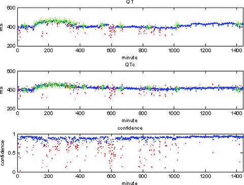
QT_c interval shows prolongation after drug dose (sotalol). Green markers from discrete BioQT measurements on 10‐second ECG data show good agreement with continuous Holter data.

Figure 7 shows the shape analysis results for one of the subjects with a 24‐hour Holter recording in the sotalol study. Four of the templates automatically generated by the BioQT software can be seen in the figure: first, the initial template (minute 16), which is an ECG waveform with a normal T‐wave shape. Then, at minute 184, another template is generated, which reveals a reduction in the height of the T wave. When the maximum morphology change occurs (minute 388), the T wave is almost entirely flat, as evidenced by the third template. By the time of the fourth template shown in the figure (minute 568), the T wave is well on its way to having recovered its original shape.

Figure 7.

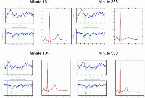
Templates generated by the BioQT on‐line algorithm, at minutes 16, 184, 388, and 568 of a 24‐hour Holter study when the subject was given a 320 mg dose of sotalol. Each template, shown in red, has the same two panels on its left: the QT interval and morphology novelty indicator, with a vertical green line indicating the time at which the template is generated. Note the flat T‐wave shape at minute 388.

For each template, the same two panels displayed to the left of the template represent the QT interval (top panel) with the morphology novelty indicator shown below, both plotted against time (for the whole 24 hours of the study). The green vertical line indicates for each panel the time at which the template is generated. The morphology novelty indicator continues to show a lower probability of normality (i.e., increasing degree of novelty) after the time at which the maximum QT prolongation is found. The greatest deviation from shape normality (the lowest value of the log likelihood for the morphology indicator) occurs at around 388 minutes into the recording, with the shallow and wide T wave of the third template.

The combined investigation of QT prolongation and T‐wave morphology changes has also been performed with recordings from subjects who were given moxifloxacin. This analysis revealed that, not surprisingly, drug‐related perturbation of the T wave is greater in subjects receiving sotalol than in those receiving moxifloxacin. The chronological dissociation of T‐wave morphology changes from the QT prolonging effect of the drug, found with sotalol, is not replicated with moxifloxacin. This can be seen from examining Figures 8 and 9 together. These figures also include a time plot of the QT/RR gradient computed, for every beat, using a sliding 4‐hour window centered on the beat in question (i.e., 2 hours of data before the beat and 2 hours afterwards. The value for the first 2 hours is simply held to be constant, set to the value of the gradient in the first 4 hours in the recording; similarly, the value for the last 2 hours is taken to be the gradient calculated for the last 4 hours).

Figure 8.

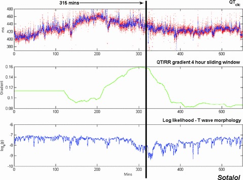
Time plots of QT_cIc (upper trace), QT/RR gradient computed over a 4‐hour sliding window (middle trace), and morphology novelty indicator (lower trace) for a sotalol 24‐hour Holter recording (double dose day). In the plot of QT_cIc, all the high‐confidence beats are shown in red; the blue trace represents the output of a 10‐point moving‐average filter. The lower trace is a plot of the log likelihood of the T‐wave morphology shape descriptor vectors. The point of maximum morphology change (315 minutes after the start of the recording) is indicated by a black vertical line.

Figure 9.

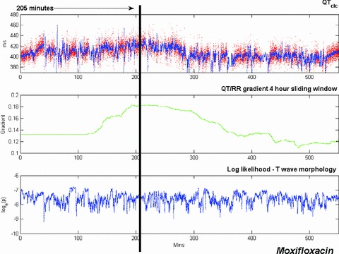
Time plots of QT_cIc (upper trace), QT/RR gradient computed over a 4‐hour sliding window (middle trace), and morphology novelty indicator (lower trace) for a moxifloxacin 24‐hour Holter recording. The point of maximum QT prolongation (205 minutes after the start of the recording) is indicated by a black vertical line.

Interestingly, the peak change in the QT/RR gradient for the sotalol data (Fig. 8) occurs at approximately the same time as the maximum morphology change (315 minutes into the recording for this subject), not at the time of maximum QT prolongation, which takes place much earlier. With the moxifloxacin data, the recording was considerably noisier but a small increase in QT_cIc is still discernible in the upper trace in Figure 9. The maximum increase in QT_cIc occurs 205 minutes after the start of the recording, just after the peak change in QT/RR gradient computed over the 4‐hour sliding window. The morphology indicator is oscillatory throughout the moxifloxacin recording, as the recording is noisy and there are no significant changes in the shape of the T wave.

As mentioned in the Methods section, BioQT provides not only a fully automated analysis, with confidence values, of QT prolongation and T‐wave morphology changes for each beat in a 24‐hour drug study, it also includes a software tool which allow a cardiologist to review and then reannotate or reject the templates automatically generated by the on‐line templating algorithm.

An example of the use of this software tool is shown in Figure 10. The top graph shows the template in black, with the family of beats used to generate it in light gray. All the beats in gray have been warped onto the template time axis using DTW. The cardiologist can adjust the position of the annotation lines either by dragging the vertical lines with the mouse or using the cursor arrow keys on the keyboard to move by one pixel at a time. The currently active annotation (which moves with the arrow keys) is shown highlighted with its indicator in red (here T_off).

Figure 10.

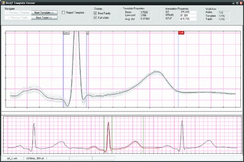
Display screen for the BioQT expert reannotation tool. The upper graph shows the template in black, with the family of beats used to generate it in light gray, and expert annotation lines as vertical blue lines. The currently active annotation is shown highlighted with its indicator in red at the top of the graph (T_off). The lower trace shows the template warped onto the middle beat of a triplet of beats.

The lower trace in Figure 10 shows a triplet of beats, the middle beat being one of the beats used to generate the template. The red trace shows the template warped onto the beat's time axis (the reverse mapping from the top graph). When the cardiologist moves the annotations, the corresponding positions on the lower trace (the green vertical lines) also move according to the DTW mapping.

An example of the use of the reannotation tool is shown in Figure 11. The upper trace in this figure shows the QT interval measurements for a 24‐hour Holter recording taken from a moxifloxacin study in which there are two periods in the study (shown shaded in Fig. 11) during which most of the beats have an unusual morphology. The confidence values associated with these beats are below the rejection threshold of 0.7 and so the QT interval measurements are not displayed. Once the cardiologist has reviewed and reannotated the templates generated during these periods, each beat is automatically reannotated using reverse DTW, producing the refined analysis of the lower trace, in which the reannotated beats are reinserted into the QT interval time‐series.

Figure 11.

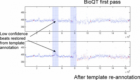
BioQT analysis of moxifloxacin 24‐hour Holter recording. The upper trace shows the first‐pass analysis of QT interval values, with missing beats (due to low confidence) in the two shaded sections. After the cardiologist has reannotated the templates from these sections, each beat is automatically reannotated and its QT interval measurement is reinserted into the interval time‐series, as shown in the lower trace.

The refined analysis enabled by the BioQT reannotation tool has now been applied to placebo and moxifloxacin 24‐hour Holter recordings from a definitive QT study performed in normal human volunteers. QT interval values were calculated as 5‐minute averages at each time point and were compared to cardiologists’ manual results obtained by measurement of three consecutive beats in each of three ECGs performed at each time point (standard ECG data). The results are given in Table 1. Standard deviation (SD) values are shown for each time point for the placebo and moxifloxacin arms. The percentage increase of SD of QT_c for the standard manual method with respect to the SD obtained by the BioQT method is given in Table 1. SD by the manual method was higher at every time point. The average increase was 44% and 30% for the placebo and moxifloxacin treatments, respectively. The improvement in SD delivered by the BioQT refined analysis indicates the potential for reducing sample size requirements in definitive QT studies analyzed using this method.

Table 1.

Standard Deviation (SD) Values for QT_c Values in the Placebo and Moxifloxacin Arms of a Definitive QT Study

Hour	Placebo			Moxifloxacin
	Refined HMM	Standard ECG	%	Refined HMM	Standard ECG	%
0.5	5.62	9.92	77	6.59	9.69	47
1	7.37	8.18	11	8.66	9.56	10
2	7.47	11.13	49	7.39	11.12	50
4	7.06	10.45	48	9.19	9.92	21
12	9.35	12.68	36	9.75	11.92	19
		Average%	44		Average%	30

The SD of QT_c for the refined Hidden Markov Model (HMM) of BioQT is shown in the left‐hand most column for both arms. The SD of QT_c for the standard manual method is shown in the middle column. The percentage increase in SD obtained with the standard manual method with respect to the SD obtained by the BioQT method is given in the third column.

CONCLUSION

The BioQT probabilistic model provides fully automated QT analysis, with confidence values for self‐checking, on very large data sets such as 24‐hour 12‐lead Holter recordings. The technique has shown itself to be capable of detecting drug‐induced changes in cardiac repolarization status in humans, characterized by both QT interval prolongation and T‐wave shape changes. In addition, the refined analysis made possible by automatic templating and expert reannotation of a small number of templates potentially leads to a reduction in the sample size requirements for definitive QT studies.

Conflicts of Interest:  Lionel Tarassenko is a non‐executive director of OBS Medical, and holds stock in the company. Mustafa Poonawala is Vice President of Engineering at OBS Medical and holds stock in the company. Jay Mason is Chief Medical Officer at OBS Medical.

REFERENCES

- 1. Kass RS, Moss AJ. Long QT syndrome: Novel insights into the mechanisms of cardiac arrhythmias. J Clin Invest 2003;112:810–815. [DOI] [PMC free article] [PubMed] [Google Scholar]
- 2. International Conference on Harmonisation . Guidance on E14 Clinical Evaluation of QT/QTc Interval Prolongation and Proarrhythmic Potential for Non‐Antiarrhythmic Drugs; availability. Notice Fed Regist 2005;70:61134–61135. [PubMed] [Google Scholar]
- 3. Laguna P, Jane R, Caminal P. Automatic detection of wave boundaries in multilead ECG signals: Validation with the CSE database. Comput Biomed Res 1994;27:45–60. [DOI] [PubMed] [Google Scholar]
- 4. Xue Q, Reddy S. Algorithms for computerized QT analysis. J Electrocardiol 1998;30:181–186. [DOI] [PubMed] [Google Scholar]
- 5. Hughes NP, Tarassenko L. Probabilistic models for automated ECG interval analysis in Phase 1 Studies. Technical Report BSP 08‐01, Available at http://www.robots.ox.ac.uk/~davidc/pubs/bsp_08_01.pdf. [Google Scholar]
- 6. Shensa MJ. The discrete wavelet transform: Wedding the a trous and Mallat algorithms. IEEE Trans. Signal Process 1992;40:2464–2482. [Google Scholar]
- 7. Rabiner LR. A tutorial on hidden Markov models and selected applications in speech recognition. Proc IEEE 1989;77:257–286. [Google Scholar]
- 8. Hughes NP. Probabilistic Models for Automated ECG Interval Analysis. DPhil thesis, University of Oxford , 2006.
- 9. Bishop CM. Pattern Recognition and Machine Learning. Springer, 2006. [Google Scholar]
- 10. Holmes JR, Holmes W. Speech Synthesis and Recognition, 2nd Ed London : Taylor and Francis, 2001. [Google Scholar]
- 11. Sarapa N, Morganroth J, Couderc JP, et al Electrocardiographic identification of drug‐induced QT prolongation: Assessment by different recording and measurement methods. A.N.E. 2004;9:48–57. [DOI] [PMC free article] [PubMed] [Google Scholar]