

Abstract
Small‐angle scattering (SAS) of X‐rays and neutrons is a fundamental tool to study the nanostructural properties, and in particular, biological macromolecules in solution. In structural biology, SAS recently transformed from a specialization into a general technique leading to a dramatic increase in the number of publications reporting structural models. The growing amount of data recorded and published has led to an urgent need for a global SAS repository that includes both primary data and models. In response to this, a small‐angle scattering biological data bank (SASBDB) was designed in 2014 and is available for public access at http://www.sasbdb.org. SASBDB is a comprehensive, free and searchable repository of SAS experimental data and models deposited together with the relevant experimental conditions, sample details and instrument characteristics. SASBDB is rapidly growing, and presently has over 1,000 entries containing more than 1,600 models. We describe here the overall organization and procedures of SASBDB paying most attention to user‐relevant information during submission. Perspectives of further developments, in particular, with OneDep system of the Protein Data Bank, and also widening of SASBDB including new types of data/models are discussed.
1. INTRODUCTION
The Small Angle Biological Data Bank (SASBDB, http://www.sasbdb.org) is a curated repository for bio‐macromolecular small‐angle scattering of X‐rays and neutrons (SAXS and SANS) data and models, which was released to the general public in August 2014.1 Since its inception, the number of entries in the SASBDB has steadily increased, influenced by both the open‐access movement and community‐lead standardization efforts for structural biology.2, 3 By April 2019, the number of SASBDB entries reached 1,000, with several hundred on‐hold or under review. Based on the 2018–2019 growth statistics, 32 entries are deposited into SASBDB, on average, per month from all over the world (Figure 1). Approximately, 84% of SASBDB depositions describe protein scattering experiments (purified monodisperse proteins, oligomers and mixtures, intrinsically disordered proteins [IDPs], etc.), 6% are polynucleotide (DNA/RNA) studies, 9% are heterocomplexes (protein‐polynucleotide, nanolipoprotein particles, etc.) while the remaining 1% include “non‐standard” bioSAXS investigations, for example, squid eye lenses.4 Of the deposited SAS entries, 93% were measured on synchrotron radiation facilities, 5% using in‐house X‐ray laboratory instruments, and less than 2% using neutrons. Aside from the deposition of scattering data and the extracted structural parameters (e.g., the radius of gyration R g, volume, molecular weight MW, and maximum particle dimension D max estimates) 71% of SASBDB entries also include additional modeling. Approximately 24% of entries have only ab initio bead models; 41% of data sets are fitted using hybrid atomistic/rigid‐body models, often in combination with ab initio modeling, while 8% are fitted using ensemble‐model approaches (Figure 2). Most of the released SASBDB entries (96%) are linked to published manuscripts via a DOI or a PubMed identifier.
Figure 1.
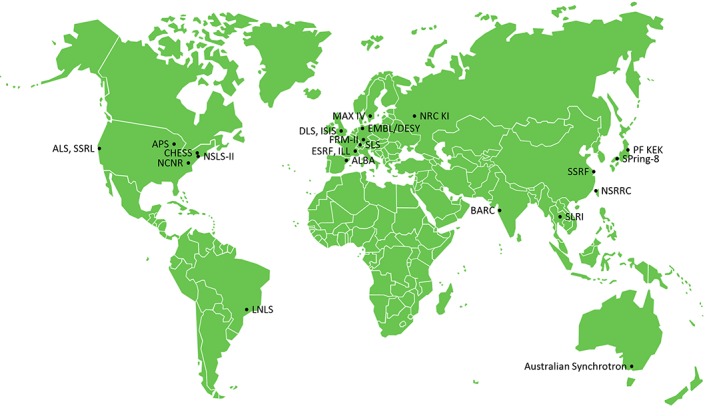
Large scale synchrotron radiation and neutron facilities contributing to SASBDB
Figure 2.
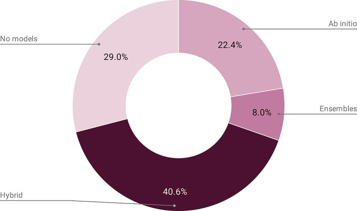
SASBDB contents by model type
The data and models deposited in SASBDB as well as metadata accompanying each entry (e.g., sample conditions, instrument parameters, protein sequence(s), links to UniProt and the Protein Data Bank [PDB], etc.) are fully and freely available. Users of SASBDB should attribute the original authors in any subsequent work. SASBDB is a curated data bank whereby the data, models and the additional metadata for each entry are manually reviewed for quality assurance. Their release is dictated by the depositor whose work has typically undergone, or is undergoing, peer‐review from journal referees who can request access to the pre‐released SASBDB depositions. If a manuscript is accepted or published, the accompanying SASBDB entries are released and linked to that manuscript. SASBDB, while adhering to the recommended SAS publication guidelines in structural biology,3 does not make decisions on data interpretation or data quality, but now reports a set of validation metrics to help assessing each entry.
2. SASBDB DATA PRESENTATION
A SASBDB entry page is divided into two main sections. The upper section displays the project, or manuscript title and authors (with DOI and PubMed links to the manuscript), the title of the individual entry as well as the primary scattering data, associated plots, and structural parameters. The lower half shows model‐fits and models that the depositor may have provided, in combination with a text description of the entry (including relevant observations reported by the depositor during deposition) plus the sample and macromolecule definitions, for example, the FASTA sequence for proteins and links to UniProt or the PDB.
The experimental scattering data are presented for each entry page using three plots:
The primary scattering data is shown as a log‐linear plot (log I(s) vs s, where I is the scattering intensity and s = 4πsinθ/λ, 2θ is the scattering angle, λ is the wavelength), a commonly accepted way to represent 1D biological SAS data (Figure 3e). The log‐linear representation helps one to visualize both very‐low, mid‐range, and higher‐angle data simultaneously.
A Guinier plot, ln I(s) versus s 2 (Figure 3p) at low values of s. Guinier 5 showed that the scattering intensity at very low angles is dependent on the R g and forward scattering at zero angle I(0). For monodisperse systems of non‐interacting particles, the Guiner plot in the range s min R g < 1.0 ∼ 1.3 should be linear, the slope relating to the R g and the extrapolated to s = 0 intercept, to the I(0). Upward deviations from linearity in the Guinier plot suggest that attractive interactions, or aggregates, are present within the sample; negative deviations suggest repulsive (charged) interactions between particles. A vertical blue line at sR g = 1 acts as a reference, to evaluate whether the data have been measured to sufficiently low‐angle to capture the Guinier region. The parameters from the Guinier approximation (reported on the plot) may be cross‐checked against those obtained from p(r) vs r (see below) and the I(0) in combination with the sample concentration provides the experimental MW estimate.
A dimensionless Kratky plot of (sR g)2 I(s)/I(0) versus sR g (Figure 3q) to qualitatively estimate of compactness of a macromolecule. A bell‐shaped peak in the plot, with a maximum of 1.104 centered at sR g = √3 indicates that the particle is likely globular or compact, while the development of a plateau, followed by an increasing linear trend in the plot for sR g > √3 indicates that less compact state(s) are present in solution (e.g., flexible linkers, unfolded proteins or highly anisometric particles).6
Figure 3.
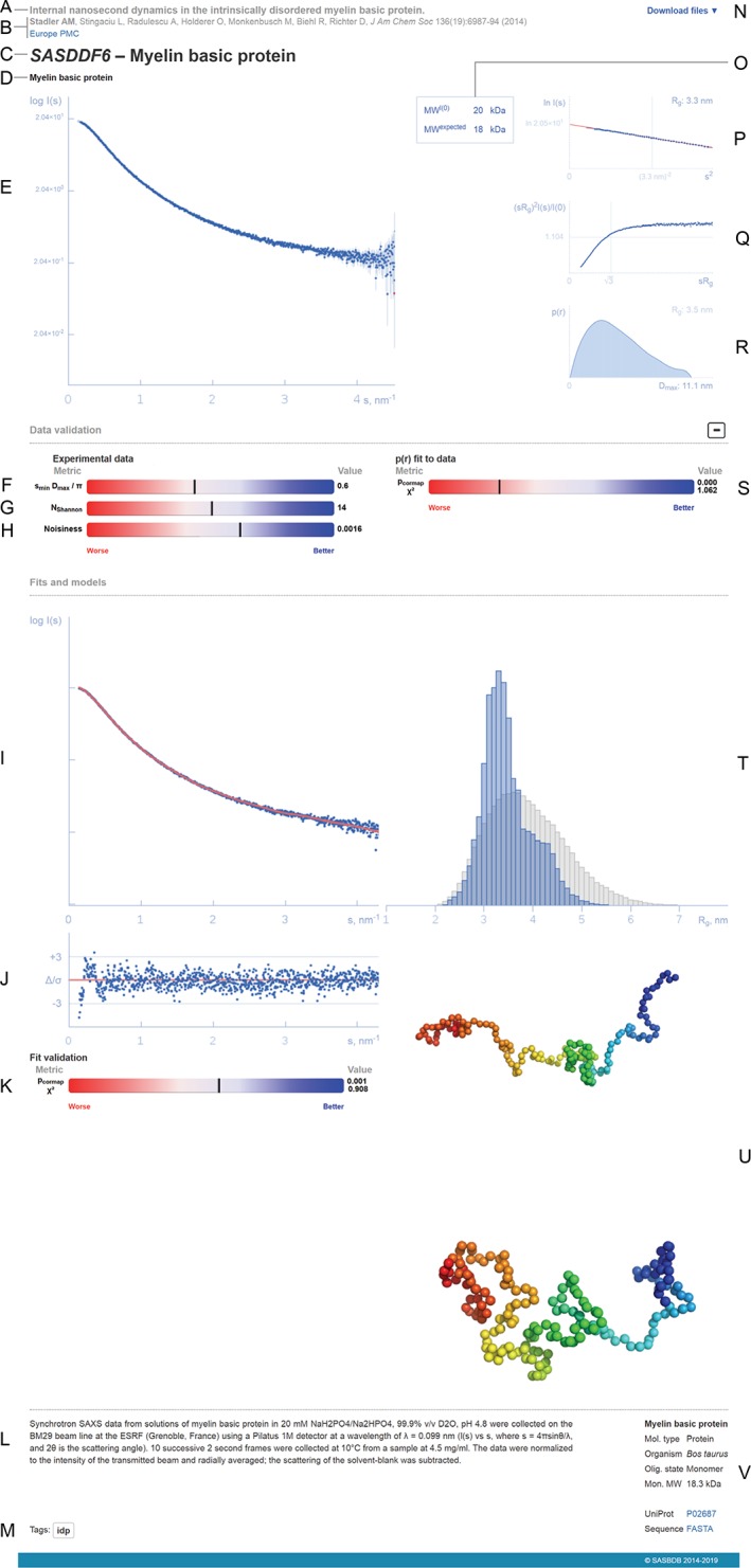
Representation of a SASBDB entry (based on https://www.sasbdb.org/data/SASDDF6/). (a) Title of the publication (or project in case of unpublished data). (b) List of authors (the main contributor is highlighted in bold), journal reference and a link to Europe PubMed Central. (c) SASBDB code and the title of the entry. (d) Names of the macromolecules that were measured. (e) Experimental scattering data (logarithmic plot). (f, g) Experimental data range percentile ranks. (h) Experimental noise percentile rank. (i) Fit to the experimental data. (j) Error‐weighted residual difference plot. (k) Goodness‐of‐fit percentile rank. (l) Experimental details. (m) Entry tag. (n) Drop‐down list of files available for download. (o) Comparison between experimental and expected molecular weights. (p) Guinier plot with the linear fit and the estimated values of the forward and scattering I(0) and the radius of gyration R g. (q) Dimensionless Kratky plot. (r) Pair distance distribution function p(r) and the maximum intraparticle distance Dmax. (s) p(r) goodness‐of‐fit to data percentile rank. (t) Histogram of the R g distribution of the generated pool (grey bars) compared to the final ensemble (blue bars), if present. (u) Associated models, for example, the most representative models from EOM ensemble. (v) Biological details of each measured macromolecule, FASTA sequence and link to UniProt
In addition, the distance distribution function p(r) vs r profile is also displayed and the R g and D max calculated from p(r) are reported (Figure 3r). The expected MW, calculated from the deposited sequence and ligand information is also displayed along with the SAS‐determined MW,7, 8 or, alternatively, those from other biophysical techniques, for example, multi‐angle laser light scattering (MALLS), analytical ultracentrifugation (AUC) or mass spectrometry (MS). SASBDB does not generally accept MW estimates derived from “standardized SEC columns” without justification (e.g., described below in the “Description box” of STEP 2 of the deposition process) as these estimates are often inaccurate.
The lower half of the entry page presents the models and fits uploaded by the depositor, that include ab initio bead models for example,9, 10, 11 as well as atomistic models, for example, derived from hybrid rigid‐body modelling.12, 13, 14 Single‐model representations may be used to describe the scattering data measured from monodisperse, ideal samples, while the information from polydisperse solutions can be represented by a volume‐fraction weighted cohort of multiple models. The number of models can be small (2, 3) e.g., for oligomeric equilibrium mixtures, or significantly large of for example, in for IDPs. In the latter case, distributions of conformational states selected from the initial (semi‐randomized) generated pool is usually the main outcome of the analysis. The R g distribution of the refined pool, for example, using ensemble optimization method (EOM)15 or minimal ensemble search (MES)16 is compared to the R g histogram of the initial structural states. This comparison provides insights into the flexibility of the system in solution. The SASBDB accepts the R g distributions file in a plain text format (Figure 3t) and the depositors have the option of uploading “ensemble model representatives” and relevant log files (Figure 3u). Large (several hundred, or thousand models, for example, from molecular dynamic [MD] simulations) may be included as an additional zip‐file upon agreement with the SASBDB curators.
3. DATA DEPOSITION INTO SASBDB THROUGH WWW.SASBDB.ORG
The SASBDB accepts SAS data measured from biological materials, primarily 1D radially averaged isotropic scattering data from dilute macromolecular solutions after subtraction of solvent or buffer scattering. At present, the deposition interface is set up for the upload of these types of data, although it is also possible to cater for “non‐standard” scattering projects, for example, bio‐nanoconjugates, nanoparticles, biological gels, etc. The experimental data, metadata, and models are deposited via the Web user‐interface after a simple registration process. The interface helps to ensure that the data submitted are consistent with the requirements outlined by the wwPDB small angle scattering task force (SAStf)17 and the publication guidelines.3
After an entry is submitted to SASBDB it is reviewed manually by the curators. If revisions are necessary, the depositor will receive a request to revise‐and‐resubmit their data incorporating the requested changes. If an entry is considered complete and accepted, a SASBDB accession code is assigned and no further changes to that entry are allowed via the deposition interface to ensure that a 1:1 correspondence is maintained between a SASBDB deposition and its corresponding accession code. Revisions to code‐assigned SASBDB entries, for example, that may be requested by an external peer‐reviewer, are dealt with manually via correspondence between the depositor and one of the SASBDB curators, thereby maintaining the integrity of the data bank.
Any SASBDB entry assigned an accession code remains by default “on‐hold,” i.e., protected via a key‐string encoded link and will not appear in the publicly accessible SASBDB interface. It is over to the depositor to privately disseminate this on‐hold link with colleagues, journal reviewers/editors, etc. who can then view the on‐hold entry without signing in to SASBDB. Data associated with work that has not been published will not be released until approved by the principal contributor, or nominally after 6 months on hold at which point a request to release the entry is made or an extension granted. The depositor may release unpublished data at any time; publication is not mandatory for making data publicly available.
3.1. The deposition procedure
A step‐by‐step guide is available on the SASBDB website to aid users through the deposition process (see https://www.sasbdb.org/media/SASBDB_deposition_guide.pdf). The deposition process begins with setting up a project followed by four deposition steps. Listed below are the sections that we have found to be the most troublesome for SASBDB depositors, with points of clarification.
3.2. SASBDB project
A project is a single‐set, or combined group, of scattering data and models related under a commonly shared or single title, for example, a set of results obtained for a specific publication, manuscript in preparation, etc. The advantage of the project system is that multiple SASBDB entries can be pooled under one title and, when released, further linked automatically, for example, to a published manuscript. A project can be accessed by its own URL (either confidentially as an on‐hold link, or as a public link after release) and will list all relevant SASBDB codes. Clicking on the project title will list all SASBDB entries relating to that project or manuscript. The project URL helps, for example, to communicate multiple SASBDB accession codes to journal referees, or to report several individual SASBDB accession codes (often requested by journals), or when searching for all entries relating to a specific investigation on the SASBDB website. When setting up a project it is not advised to pool the results from a single macromolecule spanning multiple investigations under one common macromolecule project title. For example, 28 alcohol dehydrogenase SAXS data sets have been collected spanning seven separate investigations; this scenario would be categorized as seven projects, not one ‘alcohol dehydrogenase’ project.
Another way of grouping SASBDB entries is the tagging system. A tag is a keyword or term assigned to a SASBDB entry representing a certain feature, for example, “intrinsically disordered protein,” “DNA,” “SANS,” etc. This kind of metadata helps describe an entry and allows it to be found again by browsing or searching. Tags are generally chosen by the annotators from a controlled vocabulary, however, the depositors may suggest new tags.
3.3. STEP 1: Sample title, sample macromolecules, ligands and buffer (solvent) information
The upload of correct metadata linked to a set of experimental results is the major cause of delay in processing SASBDB entries, including the information requested in STEP 1 (additional metadata is also requested in STEP 3, see below).
3.3.1. Define the sample title of an entry, name and category of the macromolecule
For proteins, SASBDB adheres as much as reasonably possible to include the recognized UniProt protein name in the title of a SASBDB entry (in those instances where a protein sequence, and associated source organism, has been deposited into UniProt, http://www.uniprot.org).18 For purely synthetic proteins, or those without UniProt codes depositors may use title descriptors at their discretion. Incorrectly annotated UniProt entries should be dealt with between the depositor and UniProt (SASBDB does not contribute to annotating/correcting UniProt entries).
3.3.2. Correct protein or DNA/RNA sequences
Delays may also be caused by uploading the incorrect protein or DNA sequences. First, the actual sequence of the macromolecule should always be uploaded, for example, a protein sequence that includes all N‐terminal or C‐terminal affinity tags and the associated oligomeric state. Second, for proteins, the amino acid sequence should undergo an alignment against those sequences in UniProt to obtain the amino‐acid range of the protein construct used for the scattering experiment relative to the native sequence in UniProt. If the UniProt code is already known, the UniProt link and the FASTA sequence of the protein can be automatically fetched from the SASBDB deposition interface utilizing UniProt application programming interface (API) service. The expected MW is automatically calculated from the amino acid or DNA/RNA sequence taking into account the oligomeric state of the macromolecule. It is up to the user to explain any significant difference between this expected/calculated and the experimentally determined MW from the scattering data. Significant/unexplainable MW discrepancies may result in a revision request prior to ascribing a SASBDB accession code.
There is now an option to define ligands, lipids or other bound molecules using the “add molecule” interface at STEP 1. The chemical formula of the bound small‐molecule or ligand and the stoichiometry are required to include these molecules in the “expected MW” calculation.
3.3.3. Buffer information
The chemical formulae of the buffer components of the solvent used for background scattering correction/subtraction should be uploaded.
3.4. STEP 2: Upload of scattering data and structural parameters
The reduced and background subtracted scattering data are typically provided in three‐column format as follows: momentum transfer (s), the intensities (I(s)) and the error (standard deviation) on the intensities, σ(I(s)), where s is in nm−1 or Å−1 and I(s) is in arbitrary units (a.u.) or on an absolute scale (cm−1) (these units can be selected). However, and importantly, the structural parameters typed into the boxes in STEP 2 must be in nm units (e.g., the estimated Guinier R g), and the MW estimated in kDa. The Porod volume is recorded in nm3.
The uploaded data are automatically checked for “over‐subtraction,” i.e., systematically negative portions which may have been a result of a mismatch between buffer composition of solution and solvent. If a statistically significant negative data range is detected by an embedded algorithm, a warning message on a possible over‐subtraction is shown.
There following “types of curve” can be selected and deposited:
“single concentration” (batch measurement);
“merged” data (batch measurement, combined concentration series);
“extrapolated to infinite dilution” (concentration series extrapolation);
“SEC‐SAS” (size‐exclusion chromatography coupled to SAXS or SANS measurements);
‘co‐flow batch measurement;
“co‐flow SEC‐SAS” (size‐exclusion chromatography coupled to SAXS measurements).
The pair distance distribution function p(r) may also be uploaded at STEP 2. Several file formats are available for the p(r) file(s), including ATSAS GNOM,19 BayesApp,20 BioXTAS RAW,21 GIFT22 and ScÅtter. Files in GNOM format are automatically parsed for the structural parameters; for p(r) files of other formats, the parameters are calculated on the fly.
Finally, a description box is provided at STEP 2 to add relevant text information (e.g., entry SASDCA323 provided a detailed account to clarify experiment details). This box, still underutilized by SASBDB depositors, is an important resource in the manual curation to avoid extra questioning, revisions and delays. Examples include cases where a depositor deliberately wants to show a model that does not fit the data, or where the quoted “experimental MW” is derived from another biophysical technique, for example, MALLS or AUC.
3.5. STEP 3: Defining the instrument parameters used for the SAS experiment
This step causes the most problems for SASBDB depositors in terms of finding and locating the information required for the deposition such that most revision requests to depositors come from having ignored STEP 3. The basic instrument parameters asked are as recommended:3
the date the experiment was performed;
the instrument and detector used (now available as a drop‐down list of over 85 instrument/detector combinations);
the radiation wavelength (in nm);
the sample to detector distance;
the cell temperature (or sample exposure temperature);
the storage temperature of the sample (prior to exposure);
the exposure time and number of data frames used to generate the final scattering profile;
the sample concentration (or concentration range in the case of merged or extrapolated to infinite dilution options).
Additional options for SEC‐SAS are:
the type of SEC column used (from a dropdown list of 19 options; more can be added);
the sample injection concentration;
sample injection volume;
SEC flow rate.
At present, it is very difficult to parse this information directly from the data files uploaded to SASBDB. Some facilities or instrument outputs simply do not record this information in the data files; other facilities use non‐human readable or “instrument jargon” to embed the parameters in long lists of other information in the data file header or footers. In cooperation with several large‐scale facilities, SASBDB works on including these parameters in a standard “parsable” format to easily find this information during deposition.
3.6. STEP 4: Upload associated model and model‐fit files
SASBDB attempts to accept fit files and model files generated using different software packages that can be selected during the upload process. At present, there are approximately 20 model‐fit program options and over 35 modeling programs that depositors can choose using a dropdown list. These include the programs of the ATSAS suite,24 FoXS,25 MultiFoXS26 and WillItFit27 as well as modeling programs such as 3D‐DART,28 AllosMod,29 Cluspro,30 elNémo,31 GROMACS,32 iTASSER,33 Phyre2,34 and others. On upload to SASBDB, the model fit files (.dat, .fit, and .fir, that are typically in the column format of s, I(s), σ(I(s)), and model(I(s))) are parsed and the goodness of fit is estimated (see “Validation of experimental data and models” below). At present, SASBDB accepts atomic or dummy‐atom coordinate files and electron density‐volume models; there are plans to accept models of other types. Direct links to the PDB entries can be established by the depositors during the upload of models to SASBDB.
3.7. Preview page, just before submission
After the models and fits have been uploaded, the depositor has a chance to review their entry prior to submission via a preview page. It is crucial to check that:
the scattering data, Guinier and dimensionless Kratky plots (automatically generated in STEP 2), as well as the p(r) profile, are displayed correctly;
the experimental data has no over‐subtraction warning. If so, it might be a cause for the SASBDB curators to ask for revisions;
the expected MW is close the experimentally determined one and the Porod volume makes sense with respect to this MW;
the model‐fit files uploaded to SASBDB relate to the fit of the model to the primary SAXS data of the entry. It is common practice that depositors upload their primary data and then use different variants (or different data) for calculating p(r) vs r and the model fits;
the molecule name, UniProt ID (for proteins), FASTA sequence and links to the PDB, if relevant, are present and
any description text is included to clarify points about the content of deposition.
If a mistake is detected, or self‐revision is required before submission, depositors can return to previous steps without risking the loss of already‐uploaded information and make the appropriate changes. The deposition may remain for as long as the depositor wants in “draft” status and the links to the draft project can be shared privately with others.
3.8. Data deposition into SASBDB via the world‐wide PDB OneDep system
If a structural biologist has obtained high‐resolution X‐ray or neutron diffraction data, NMR spectroscopy or electron microscopy data, then it is possible while depositing these data and associated models through the wwPDB OneDep System (https://deposit-2.wwpdb.org/)35 to upload a SAS project directly into SASBDB. The reverse procedure, that is, depositing high‐resolution data and models into the PDB from SASBDB is not possible, and also stand‐alone scattering projects cannot be uploaded via OneDep. When both the high‐resolution and SAS projects are deposited in parallel, SASBDB accession codes will be issued immediately, that is, the SASBDB “biocuration and wait” procedure is by‐passed. However, OneDep SASBDB depositions are checked and any revision requests are dealt with via correspondence between SASBDB and the OneDep depositor. Importantly, it is not possible for the SASBDB to release an OneDep scattering project to the public interface until the PDB has released the associated high‐resolution deposition.
3.9. Adding files or revising entries after SASBDB codes have been assigned
Sometimes, depositors require revisions to an entry after a SASBDB code has been assigned, or the addition of information or files for an entry, for example, the results obtained from SEC‐MALLS, MD simulations, advanced SANS with contrast variation analyses (e.g., Stuhrmann plots), etc. These revisions or additional files can be made and included for download in the full entry zip‐archive for a particular entry via correspondence with a SASBDB curator.
4. VALIDATION OF EXPERIMENTAL DATA AND MODELS
An advantage of a curated data bank over a passive database, which simply stores data, is that it is possible to provide/analyze feedback characterizing an individual entry relative to other entries and also to highlight potential challenges going forward by means of global statistical analysis. For example, assessment and reporting of the quality of the deposited scattering data, its information content and the reliability of model‐fitting and other types of data‐fitting are useful for SASBDB depositors and external reviewers. To facilitate interpretation of the data and to compare the quality of individual SASBDB entries we follow the principles described in36 and calculate percentile ranks for a number of key metrics. Presenting these quality scores using “worse‐better” sliders was adopted by the PDB and permits the users/reviewers to readily assess the data quality. The data validation metrics currently available in SASBDB include the measured angular data range, the level of experimental noise and, where relevant, the quality of the goodness of fit computed from the p(r) and from the models to the experimental data.
The number of useful Shannon channels in a dataset10 is automatically estimated and shown in SASBDB for all data where D max has been reported (Figure 3g). The procedure yields the highest value s max of the dataset which still contains useful information and characterizes the information content of the SAS data. It is further important that the minimum value s min provides information about sufficiently long distances to reliably determine the R g, D max and volume. The position of the first Shannon channel is s 1 = π/Dmax and the value s min D max /π is used as a metric to evaluate whether sufficient low‐angle data is available (shown as a SASBDB slider, see Figure 3f).
The experimental noise is another crucial parameter but, unfortunately, it is not uncommon that the experimental errors are wrongly estimated or absent in the user data. We had to introduce a noise estimation metric based on a single experimental curve without relying on the provided experimental errors. For this, the data are normalized and extrapolated to I(0) = 1 using the Guinier approximation, rebinned onto a common regular grid with a sampling period Δs and cropped to a common s‐range. Further, the data are Fourier‐transformed to real space up to r max = π/Δs. The distances less than D max are removed and inverse Fourier transform is applied to the truncated data to estimate the pure noise without the I(s) signal. The standard deviation of the noise is used as a lower bound estimate of the experimental noise and is reported in the respective slider (Figure 3h).
Two approaches are applied to estimate the quality of the fits calculated from the p(r) functions and from the deposited models. The classical reduced χ 2 goodness‐of‐fit test is applied when experimental errors are available; if they are not present, SASBDB attempts to parse the fit file header for the χ 2 value. To overcome the problem of missing or wrongly estimated errors an alternative approach suggested by Franke et al.37 is applied to rank the entries by the Correlation Map p‐value (Figure 3m,s). A graphical representation of deviations between the fit and the experimental data is presented in the form of error‐weighted residual difference plot (Figure 3l), as recommended by Trewhella et al.3
4.1. The challenge of experimental errors
With over 1,000 scattering profiles deposited, it is possible to obtain an overview and highlight trends based on the above validation metrics. One trend stands out above all others: the correct specification of experimental errors and the impact this has on data fitting. A quick analysis across SASBDB suggests that experimental errors are often poorly defined, both for the data from large scale facilities and lab sources.
From a total of 1,059 SASBDB entries (released and unreleased) where χ 2 and CorMap P‐values are available or relevant, 35% of entries have a χ 2 between 0.8 and 1.2 (expected range of good fit). For the rest 65% entries, the reported χ 2 is outside this range (either above or below), reaching the values as low as χ 2 = 0.0036 and as high as χ 2 = 122.
The situation is better for the CorMap test, where 64% of entries have a p‐value between .01–1.0 (a good fit); for 36% of entries the p‐value is below .01 (pointing to systematic deviations, see Figure 4, inset). Out of the 64% good fits only 42% of entries have the expected χ 2 between 0.8 and 1.2 (Figure 4, green bars); 28% of entries have overestimated errors (χ 2 < 0.8), 30% have underestimated errors (χ 2 > 1.2). What this demonstrates is that experimental errors are likely not specified correctly on a very regular basis. How error misspecification affects data interpretation is open for discussion; here, we simply report the observable trends in SASBDB.
Figure 4.
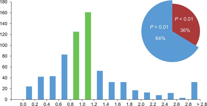
Histogram of χ2 distribution of p(r) fits with CorMap test p‐values >.01 (64% of all data sets). The green bars represent 42% of entries with expected 0.8 < χ 2 < 1.2. Inset: the ratio of acceptable p(r) fits (p‐values >.01, blue) and fits with systematic deviations (p‐values <.01, red) according to the CorMap test
5. SASBDB APPLICATION PROGRAMMING INTERFACE
The RESTful API (https://www.sasbdb.org/rest-api/docs/) was implemented in 2016 to provide programmatic access to all information stored in SASBDB in JSON, XML and sasCIF formats. The API makes it possible to retrieve a list of all publicly available SASBDB entry codes, entries filtered by a molecular type (protein, DNA, RNA, etc), or a set of entries marked by a specific SASBDB tag. The whole set of data stored in SASBDB is easily available by entry code. This includes all the URLs to data files and plots as well as specific entry metadata.
A specific private API was designed to enable submission of SASBDB entries as part of a PDB OneDep deposition session38 for X‐ray, NMR or cryo‐EM structures where SAS was used as a supporting technique.
6. IMPLEMENTATION
SASBDB is implemented in Python 2.7 (http://www.python.org/) using Django 1.11 as a web framework (http://www.djangoproject.com) and the relational database MariaDB 10.1 (http://mariadb.com). The SAS data analysis suite ATSAS 2.824 is used for data validation. The combination of Celery 4.3.0 (http://www.celeryproject.org) and RabbitMQ 3.6.6 (http://www.celeryproject.org) serves as a task queuing system in order to run asynchronous tasks outside of the HTTP request‐response cycle. For the search engine we use Django Haystack 2.8.1 (http://haystacksearch.org) together with Elasticsearch 2.4.5 (http://www.elastic.co). For data plotting we use gnuplot 5 (http://www.gnuplot.info), for model visualization we use PyMOL 2.2 (http://www.pymol.org/) and the interactive viewer JSmol 14.15.2 (http://www.jmol.org/).
7. OUTLOOK
After 5 years of operation, SASBDB became an important resource for disseminating experimental information and models in biological SAS. The submission rate and also the utilization of the database are constantly growing, and the recognition of SASBDB as the official deposition site by the IUCr Commission3 played a very important role. For the future developments, further modernization of the user interface is planned and better linkage to the PDB submission resources is underway to improve and encourage the OneDep line of submission. Work has also started to widen the data bank and allow for not only biological but also soft matter data/models from SAXS/SANS to be deposited (collaboration with the Technical University of Applied Sciences Lübeck, Germany).
CONFLICT OF INTEREST
The authors declare that there is no conflict of interest regarding the publication of this article.
ACKNOWLEDGMENTS
We would like to acknowledge the contribution of Daniela Schacherer to the implementation of the over‐subtraction detection algorithm.
Kikhney AG, Borges CR, Molodenskiy DS, Jeffries CM, Svergun DI. SASBDB: Towards an automatically curated and validated repository for biological scattering data. Protein Science. 2020;29:66–75. 10.1002/pro.3731
Funding information German Ministry of Science and Education, Grant/Award Number: 16QK10A ‐ SAS‐BSOFT; iNEXT, Horizon 2020 programme, Grant/Award Number: 653706
REFERENCES
- 1. Valentini E, Kikhney AG, Previtali G, Jeffries CM, Svergun DI. SASBDB, a repository for biological small‐angle scattering data. Nucleic Acids Res. 2015;43:D357–D363. [DOI] [PMC free article] [PubMed] [Google Scholar]
- 2. Jacques DA, Guss JM, Svergun DI, Trewhella J. Publication guidelines for structural modelling of small‐angle scattering data from biomolecules in solution. Acta Crystallogr. 2012;D68:620–626. [DOI] [PubMed] [Google Scholar]
- 3. Trewhella J, Duff AP, Durand D, et al. 2017 publication guidelines for structural modelling of small‐angle scattering data from biomolecules in solution: An update. Acta Crystallogr. 2017;D73:710–728. [DOI] [PMC free article] [PubMed] [Google Scholar]
- 4. Cai J, Townsend JP, Dodson TC, Heiney PA, Sweeney AM. Eye patches: Protein assembly of index‐gradient squid lenses. Science. 2017;357:564–569. [DOI] [PMC free article] [PubMed] [Google Scholar]
- 5. Wilson AJC. Small‐angle scattering of X‐rays by A. Guinier and G. Fournet. Acta Cryst. 1956;9:326. [Google Scholar]
- 6. Durand D, Vivès C, Cannella D, et al. NADPH oxidase activator p67phox behaves in solution as a multidomain protein with semi‐flexible linkers. J Struct Biol. 2010;169:45–53. [DOI] [PubMed] [Google Scholar]
- 7. Mylonas E, Svergun DI. Accuracy of molecular mass determination of proteins in solution by small‐angle X‐ray scattering. J Appl Cryst. 2007;40:s245–s249. [Google Scholar]
- 8. Hajizadeh NR, Franke D, Jeffries CM, Svergun DI. Consensus Bayesian assessment of protein molecular mass from solution X‐ray scattering data. Sci Rep. 2018;8:7204. [DOI] [PMC free article] [PubMed] [Google Scholar]
- 9. Svergun DI. Restoring low resolution structure of biological macromolecules from solution scattering using simulated annealing. Biophys J. 1999;76:2879–2886. [DOI] [PMC free article] [PubMed] [Google Scholar]
- 10. Konarev PV, Svergun DI. A posteriori determination of the useful data range for small‐angle scattering experiments on dilute monodisperse systems. IUCrJ. 2015;2:352–360. [DOI] [PMC free article] [PubMed] [Google Scholar]
- 11. Grant TD. Ab initio electron density determination directly from solution scattering data. Nat Methods. 2018;15:191–193. [DOI] [PubMed] [Google Scholar]
- 12. Petoukhov MV, Svergun DI. Global rigid body modeling of macromolecular complexes against small‐angle scattering data. Biophys J. 2005;89:1237–1250. [DOI] [PMC free article] [PubMed] [Google Scholar]
- 13. Petoukhov MV, Franke D, Shkumatov AV, et al. New developments in the ATSAS program package for small‐angle scattering data analysis. J Appl Cryst. 2012;45:342–350. [DOI] [PMC free article] [PubMed] [Google Scholar]
- 14. Kozakov D, Hall DR, Xia B, et al. The ClusPro web server for protein‐protein docking. Nat Protoc. 2017;12:255–278. [DOI] [PMC free article] [PubMed] [Google Scholar]
- 15. Bernadó P, Mylonas E, Petoukhov MV, Blackledge M, Svergun DI. Structural characterization of flexible proteins using small‐angle X‐ray scattering. J Am Chem Soc. 2007;129:5656–5664. [DOI] [PubMed] [Google Scholar]
- 16. Pelikan M, Hura GL, Hammel M. Structure and flexibility within proteins as identified through small angle X‐ray scattering. Gen Physiol Biophys. 2009;28:174–189. [DOI] [PMC free article] [PubMed] [Google Scholar]
- 17. Trewhella J, Hendrickson WA, Kleywegt GJ, et al. Report of the wwPDB small‐angle scattering task force: Data requirements for biomolecular modeling and the PDB. Structure. 2013;21:875–881. [DOI] [PubMed] [Google Scholar]
- 18. The UniProt Consortium . UniProt: A worldwide hub of protein knowledge. Nucleic Acids Res. 2019;47:D506–D515. [DOI] [PMC free article] [PubMed] [Google Scholar]
- 19. Svergun DI. Determination of the regularization parameter in indirect‐transform methods using perceptual criteria. J Appl Cryst. 1992;25:495–503. [Google Scholar]
- 20. Hansen S. BayesApp : A web site for indirect transformation of small‐angle scattering data. J Appl Cryst. 2012;45:566–567. [Google Scholar]
- 21. Hopkins JB, Gillilan RE, Skou S. BioXTAS RAW: Improvements to a free open‐source program for small‐angle X‐ray scattering data reduction and analysis. J Appl Cryst. 2017;50:1545–1553. [DOI] [PMC free article] [PubMed] [Google Scholar]
- 22. Bergmann A, Fritz G, Glatter O. Solving the generalized indirect Fourier transformation (GIFT) by Boltzmann simplex simulated annealing (BSSA). J Appl Cryst. 2000;33:1212–1216. [Google Scholar]
- 23. Pozner A, Hudson NO, Trewhella J, Terooatea TW, Miller SA, Buck‐Koehntop BA. The C‐terminal zinc fingers of ZBTB38 are novel selective readers of DNA methylation. J Mol Biol. 2018;430:258–271. [DOI] [PubMed] [Google Scholar]
- 24. Franke D, Petoukhov MV, Konarev PV, et al. ATSAS 2.8: A comprehensive data analysis suite for small‐angle scattering from macromolecular solutions. J Appl Cryst. 2017;50:1212–1225. [DOI] [PMC free article] [PubMed] [Google Scholar]
- 25. Schneidman‐Duhovny D, Hammel M, Sali A. FoXS: A web server for rapid computation and fitting of SAXS profiles. Nucleic Acids Res. 2010;38:W540–W544. [DOI] [PMC free article] [PubMed] [Google Scholar]
- 26. Schneidman‐Duhovny D, Hammel M, Tainer JA, Sali A. FoXS, FoXSDock and MultiFoXS: Single‐state and multi‐state structural modeling of proteins and their complexes based on SAXS profiles. Nucleic Acids Res. 2016;44:W424–W429. [DOI] [PMC free article] [PubMed] [Google Scholar]
- 27. Pedersen MC, Arleth L, Mortensen K. WillItFit : A framework for fitting of constrained models to small‐angle scattering data. J Appl Cryst. 2013;46:1894–1898. [Google Scholar]
- 28. Van Dijk M, Bonvin AMJJ. 3D‐DART: A DNA structure modelling server. Nucleic Acids Res. 2009;37:235–239. [DOI] [PMC free article] [PubMed] [Google Scholar]
- 29. Weinkam P, Pons J, Sali A. Structure‐based model of allostery predicts coupling between distant sites. Proc Natl Acad Sci U S A. 2012;109:4875–4880. [DOI] [PMC free article] [PubMed] [Google Scholar]
- 30. Comeau SR, Gatchell DW, Vajda S, Camacho CJ. ClusPro: A fully automated algorithm for protein‐protein docking. Nucleic Acids Res. 2004;32:96–99. [DOI] [PMC free article] [PubMed] [Google Scholar]
- 31. Suhre K, Sanejouand YH. ElNémo: A normal mode web server for protein movement analysis and the generation of templates for molecular replacement. Nucleic Acids Res. 2004;32:610–614. [DOI] [PMC free article] [PubMed] [Google Scholar]
- 32. Pronk S, Páll S, Schulz R, et al. GROMACS 4.5: A high‐throughput and highly parallel open source molecular simulation toolkit. Bioinformatics. 2013;29:845–854. [DOI] [PMC free article] [PubMed] [Google Scholar]
- 33. Yang J, Yan R, Roy A, Xu D, Poisson J, Zhang Y. The I‐TASSER suite: Protein structure and function prediction. Nat Methods. 2014;12:7–8. [DOI] [PMC free article] [PubMed] [Google Scholar]
- 34. Kelley LA, Mezulis S, Yates CM, Wass MN, Sternberg MJE. The Phyre2 web portal for protein modelling, prediction, and analysis. Nat Protoc. 2015;10:845–858. [DOI] [PMC free article] [PubMed] [Google Scholar]
- 35. Young JY, Westbrook JD, Feng Z, et al. OneDep: Unified wwPDB system for deposition, biocuration, and validation of macromolecular structures in the PDB archive. Structure. 2017;25:536–545. [DOI] [PMC free article] [PubMed] [Google Scholar]
- 36. Gore S, Velankar S, Kleywegt GJ. Implementing an X‐ray validation pipeline for the protein data Bank. Acta Crystallogr. 2012;D68:478–483. [DOI] [PMC free article] [PubMed] [Google Scholar]
- 37. Franke D, Jeffries CM, Svergun DI. Correlation map, a goodness‐of‐fit test for one‐dimensional X‐ray scattering spectra. Nat Methods. 2015;12:419–422. [DOI] [PubMed] [Google Scholar]
- 38. wwPDB consortium . Protein data Bank: The single global archive for 3D macromolecular structure data. Nucleic Acids Res. 2019;47:D520–D528. [DOI] [PMC free article] [PubMed] [Google Scholar]