SimpleDSFviewer: A tool to analyze and view differential scanning fluorimetry data for characterizing protein thermal stability and interactions

Abstract

Differential scanning fluorimetry (DSF) is a widely used thermal shift assay for measuring protein stability and protein–ligand interactions that are simple, cheap, and amenable to high throughput. However, data analysis remains a challenge, requiring improved methods. Here, the program SimpleDSFviewer, a user‐friendly interface, is described to help the researchers who apply DSF technique in their studies. SimpleDSFviewer integrates melting curve (MC) normalization, smoothing, and melting temperature (Tm) analysis and directly previews analyzed data, providing an efficient analysis tool for DSF. SimpleDSFviewer is developed in Matlab, and it is freely available for all users to use in Matlab workspace or with Matlab Runtime. It is easy to use and an efficient tool for researchers to preview and analyze their data in a very short time.

Abbreviations

DSF

differential scanning fluorimetry

DT₅₀

the temperature of half maximal denaturation

FD

first derivative

FDC

first derivative curve

HMD

half maximal denaturation

MC

melting curve

Tm

melting temperature

1. INTRODUCTION

Differential scanning fluorimetry (DSF) is a thermal shift assay method used to measure the denaturation of proteins in response to increasing temperatures, which breaks the noncovalent bonds that underlie protein folding.1, 2, 3, 4 A high temperature is required to denature a stable protein, while an unstable protein will be denatured at a lower temperature. In the DSF assay, the fluorescence of the dye Sypro Orange, which increases markedly in a nonpolar environment, is used to report the extent to which the hydrophobic sites are exposed, as the protein unfolds with increasing temperature. High temperature heating can cause protein aggregation, which leads to a drop in fluorescence. The DSF method is being adopted by an increasingly wide community, with additional applications beyond the measurement of protein stability, such as protein–ligand interactions, including those involving small molecules and drug libraries.5, 6, 7

The experiment can be done easily (Figure 1) and a large volume of data can be acquired.1, 5 The equipment requirement is modest—a common real‐time polymerase chain reaction (PCR) instrument and 96 multiwell plates. The melting curve (MC) is measured with the increase of fluorescence, and the data are exported for analysis. However, the latter can be challenging, and this currently restricts the adoption of the technique. Consequently, a program for DSF data analysis, SimpleDSFviewer, has been written to help users of DSF view and efficiently analyze their data. A number of other DSF analysis tools exist, for example, Meltdown,8 MTSA,9 TSA‐CRAFT,10 and DMAN.11 SimpleDSFviewer has a user‐friendly interface, which allows users to easily navigate its functions and preview the analyzed data. Moreover, a number of functions have been incorporated in SimpleDSFviewer, including data normalization, smoothing, and melting temperature (Tm) calculations with two convinced approaches. These are particularly useful for the analysis of noisy data and moreover generate data in export formats suitable for analysis and publication.

Figure 1.

DSF experimental pipeline. The DSF experiment can be divided into five steps: (1) preparation of the samples in a 96‐well plate; (2) measurement of the MCs with a real‐time PCR instrument; (3) export the data (raw data) into an Excel file; (4) analyze and preview the data with an appropriate software; and (5) produce publication‐quality figures with a statistical software

2. IMPLEMENTATION

SimpleDSFviewer is available as a user‐friendly graphical interface tool, which was developed in Matlab and can be run in the Matlab workspace or with Matlab runtime. The details about the code scripts are described in Data S1, Supporting Information. The DSF assays and acquisition of the exemplar data with hexahistidine‐tagged fibroblast growth factor 7 (His‐FGF7) and His‐FGF10 are described.12

2.1. Parameter selection

The temperatures including “start temperature,” “temperature step,” and “end temperature” are required if a raw data file (Figure 1A) is to be loaded. In the software, “1” signifies “Yes” and “0” signifies “No” for “Smooth,” “Normalize,” “CutMC,” and “Legend” parameters. The “Smooth” and “Normalize” parameters should be kept as “1” as the data are loaded, but the range (“Smooth Range”) can be changed to be larger or smaller. The “Normalize” and “Smooth” functions can be turned off after the data are loaded, when the original MC is desired. If the user wishes to remove the part before the protein denaturation and the part after the protein denaturation in the MC, the parameter of “CutMC” should be set as “1” before loading the data. The default values are loaded automatically and are generally suitable for analysis.

2.2. Working flow and the user interface

SimpleDSFviewer automatically processes the uploaded raw data or the sorted data (sample data format in Figure 1), as shown in the flow chart (Figure 2a). The MC data are normalized and smoothed with the given range and the first derivative (FD) of the MC is calculated. The Tm of each MC is extracted from the raw MC and first derivative curve (FDC) (Figure 2a: Output). The analyzed data may be saved in an Excel file format for further analysis. The user interface consists of four parts: data input, data modification parameters, data export, and display of analyzed data (Figure 2b). The background of the analysis is described below, and the instructions for using the software are provided in Data S1, Supporting Information.

Figure 2.

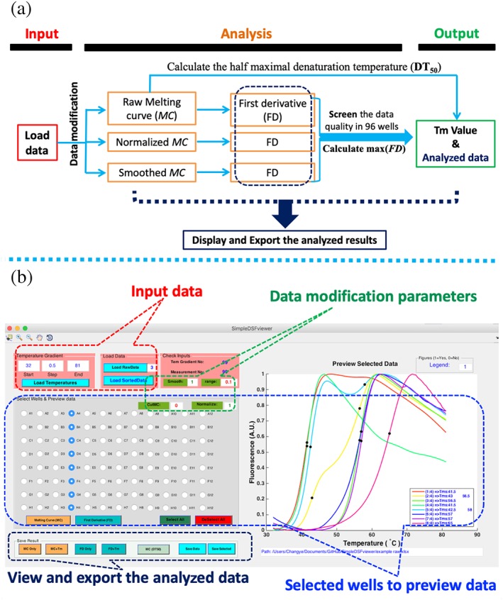
Working flow chart of the SimpleDSFviewer software and its user interface. (a) SimpleDSFviewer software contains four main parts: input data, data analysis, output, and preview of the analyzed results. The chart describes the work flow of the software. (b) User interface of SimpleDSFviewer displays four main parts to allow the users easily interact with the software: “Input data” is for uploading the raw result, “Data modification parameters” is for inputting the desired parameters, “View and Save the analyzed data” is for saving the analyzed results, and Preview box allows previewing the result of selected wells

2.3. Analysis

2.3.1. MC normalization

The background is removed by subtracting the minimum value from all points in each plotted curve, and then the MC is normalized by dividing by the maximum value in the curve (Equation 1):

$${\mathrm{MC}}_{\mathrm{norm}}=\frac{\mathrm{MC}-\min \left(\mathrm{MC}\right)}{\max \left(\mathrm{MC}\right)-\min \left(\mathrm{MC}\right)}$$ (1)

$$\mathrm{FDC}=\frac{\mathrm{MC}\left(n+1\right)-\mathrm{MC}\left(n-1\right)}{2*\mathrm{\Delta }t}$$ (2)

where MC is the melting curve value; FDC is the first derivative curve value; min(MC) is the minimum value of the MC before the protein is denatured; max(MC) is the maximum value of the MC; MC(n + 1) is the (n + 1)th value in the MC; and Δt is the difference in temperature of two neighboring measurement points.

2.3.2. MC smoothing

The MCs may be noisy, for example, due to low protein concentration, so each normalized MC is smoothed. To ensure that the original shape of the curve is maintained, each MC is smoothed in three parts, the beginning to the minimum value (before the onset of denaturation), the minimum value to the maximum value (denaturation part), and the maximum to the end (after denaturation). The smoothing method is based on Matlab's smooth function,13 and however, the smooth range can also be defined by the user. Note that the “normalization” and “smoothing” functions are optional.

To eliminate the fluorescence signal before and after the protein is denatured, the recognized fluorescence values before the protein is denatured are set to 0 and the fluorescence values after complete denaturation are set to 0.98.

2.3.3. FD calculation

The FD is calculated using Equation (2) and is normalized in the same way as the MCs.

2.3.4. Tm calculation

There are two approaches for calculating Tm values, the FD method and the half maximal denaturation (HMD) method. In the FD method, the Tm is defined as the temperature at the maximum of the FDC. The Tm calculated with the raw data and the smoothed data are almost the same, which again indicates that smoothing will not change Tm values. In the HMD method, the Tm is determined by calculating the temperature of HMD (DT₅₀), which is the temperature at which the fluorescence intensity reaches 50% of the highest fluorescence intensity. If no protein or a denatured protein is added, the returned Tm is the initial temperature (32°C in the exemplar data).

$$\mathrm{Tm}=\text{Temperature}\left(\text{maxFDC}\right)$$ (3)

$$\mathrm{Tm}=\text{Temperature}\left(\max \left({\mathrm{MC}}_{\mathrm{norm}}\right)/2\right)$$ (4)

2.3.5. Automate data screening with the findpeak function

If the MC decreases from the maximal value to the minimal value as the temperature increases, the protein is recognized as a denatured or unfolded protein. However, this may occur with proteins that have very substantial exposed aromatic residues compared to buried ones, and also with some compact proteins, that may be small or highly asymmetric. The findpeak function is used to find the peaks of the FDCs. Only when the width and height of a peak are over 10% that of the highest peak in the assay (a peak below 10% of the highest peak is recognized as noise), then the peak is recognized as a second Tm. However, if the number of recognized peaks is ≥4, the corresponding protein may be denatured, or there is no protein in the well, so Findpeak does not calculate Tm.

3. RESULTS AND DISCUSSION

3.1. Normalization and smoothing of MCs

The normalization of MCs enables MCs to be compared (Figure 3a,b). In the example, the normalization results indicate that all the curves of the three repeats (purple/green) share the same denaturation pattern and the denaturation curves are very similar. The points before and after the protein denaturation in the MC can be automatically recognized and removed from the MC, if clearer data visualization is required (Figure 3c,d). The raw MC is well represented by the smoothed curve (Figure 4a). The FDC of the raw MC can be quite noisy, which influences the calculation of Tm, but the FDC of the smoothed MC is not, thus providing a better measure of Tm (Figure 4b). The appropriateness of smoothing is demonstrated by the measurement of the differences between the raw and the smoothed data. A surface plot of these differences in the exemplar data indicates that they are very small (Figure 4c). Thus, the largest difference for the folded protein is 0.0392 (Figure 4c, flat area), and for the denatured protein it is 2.517 (Figure 4c, high peaks). Thus, smoothing can efficiently improve the data quality for calculation of FD and Tm, without changing the shape of the MC.

Figure 3.

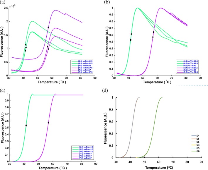
Normalization of the MCs changes the display range of measured fluorescence intensity from 0 to 1, but the shape of the MC is unaltered. (a) Original MCs of His‐FGF10 (green) and His‐FGF10 stabilized with heparin (purple). (b) Normalized MCs of the same samples. (c) The part before protein denaturation is normalized to 0 and the part after protein denaturation is normalized to 0.98. (d) The same data as (c), but with the data before protein denaturation and after protein denaturation removed. (a–d) Consist of the same data and in (c) and (d) the coincidence of the curves results in D6 masking D4 and D5 and G6 masking G4 and G5

Figure 4.

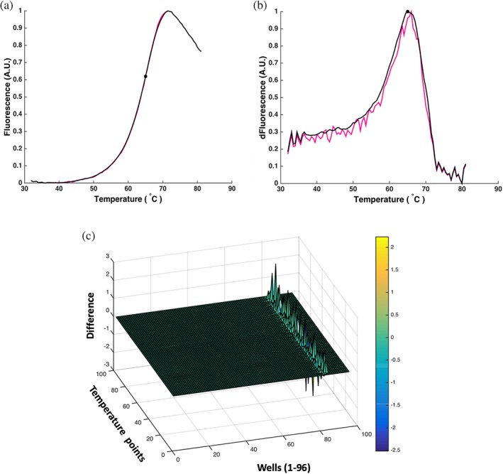
Smoothing the MCs reduces the noise level, but does not alter the shape of the curves. (a) Original MC (pink) and smoothed MC (black) of His‐FGF7 stabilized with 50 μM heparin. (b) FDCs of MCs in (a). The unsmoothed curve (pink) is a very noisy curve, while the smoothed one is not. The Tm is more accurate. (c) The differences between the smoothed and unsmoothed MC data. The normalization peaks correspond to the unfolded proteins

3.2. Tm calculation

A comparison of the Tm values calculated by the two approaches (the FD method and the HMD method) generally shows small differences in these (Figure 5a,b. The results demonstrate that the Tm values of the folded proteins calculated with smoothed data and unsmoothed data are very similar (Figure 5c), and the two analyses also give very similar Tm values for a single domain, well‐folded protein (Figure 5d). The FGF10 data provide a useful example of a behavior pattern that provides some insight into the binding reaction. Thus, at low concentrations of heparin, two protein species (i.e., free, nonstabilized FGF10 and bound, stabilized FGF10) are observed. The FD method based on the FD of the MC will present two peaks, while the HMD method only shows the shift of MC (Figure 5a,b). Thus, the HMD approach may not deal with the data appropriately when there are two protein species possessing different Tm values (Figure 5d, green circles). This may arise with ligands that do not appreciably exchange from the protein over the time of the measurement (Figure 5 and, e.g., FGF3 FGF10 and FGF2014), a protein mixture, or a fusion protein (common when a recombinant protein is unstable and requires a solubilization tag, e.g., Halo‐FGFs15). In such cases, the HMD method calculates the temperature at the half maximal denaturation position and generates a Tm value, which is an average of the two species (Figure 5d, left green circle). In contrast, the FD method takes the maximum of the FD as the Tm, and it can distinguish the peaks corresponding to the two protein species when these are reasonably separated (Figure 5). Moreover, in a small protein with substantially exposed aromatic side chains, the starting fluorescence may be the highest point, and upon heating the fluorescence declines, but then increases when the protein melts. In these instances, the HMD method cannot calculate the Tm (Figure 5d, right green circle) of the MCs with high initial fluorescence (Figure 1). Therefore, the FD method is more generally applicable. Nonetheless, determining how different the Tm values calculated by the two different methods are may provide additional information.

Figure 5.

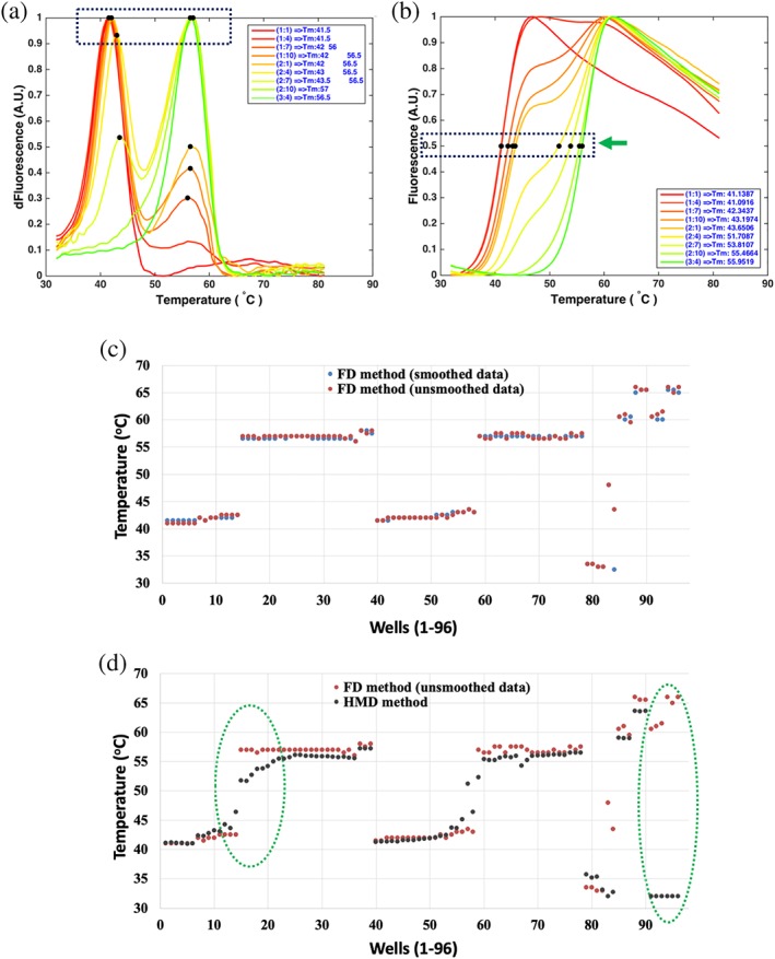
Calculation of Tm values. Two different methods are used to extract the Tm values, which are presented in figures a,b. The MCs or their first derivatives are from His‐FGF10 samples stabilized by a series of heparin ligands (concentrations are listed in Table 1). (a) The temperatures corresponding to the maxima of the FDCs are extracted as the Tm values, described as FD method. (b) The temperatures corresponding to half maximal fluorescence intensity are extracted as the Tm values, described as HMD method. (c) 96 Tm values of unsmoothed MCs and smoothed MCs were calculated using the FD method. (d) 96 Tm values of unsmoothed MCs were calculated using the FD method and HMD method. Green‐dotted circles indicate the regions of discrepancy between the two methods. The FD method is a more sensitive method for determination of curves with two Tm values (left green circle) or curves with strong starting fluorescence (right green circle)

The MC of FGF10 in 8 M urea is a declining curve and so recognized as an unfolded or denatured protein (Figure 6a). When native FGF10 was stabilized with 0.625 μM heparin, two Tm values were recognized by the FD method, a result of the heparin bound to FGF10 not exchanging readily over the time of the experiment (Figures 5 and 6a,b). The Tm values of a 96‐well plate containing unfolded and folded proteins are displayed in a heatmap (Figure 6c). The wells colored deep blue (at about the start of the color bar, Figure 6c) contain the unfolded proteins or no protein, whose Tm values are defined as the initial temperature (32°C in the exemplar data). The Tm values are presented as different colored squares from the lowest Tm (blue) to the highest Tm (red). A 3D bar plot containing the Tm values of the 96 wells is also prepared, to provide a different view of proteins’ thermal stabilities (Figure 6d).

Figure 6.

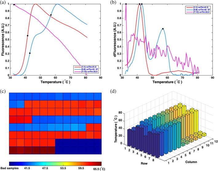
Autoscreening the MCs and preview of Tm values in 96‐well plates. Three different types of MCs in (a) can be recognized by the program. The Tm information of 96 wells is automatically presented in two figures c,d. (a) MCs of His‐FGF10 (red line), His‐FGF10 stabilized with 0.625 μM heparin (blue line), and His‐FGF10 (pink line) denatured by 8 M urea. (b) FDCs calculated from MCs in (a). (c) 2D map view of Tm values of the proteins in 96 wells. The dark blue wells contain unfolded proteins or unstable proteins (e.g., proteins in an inappropriate buffer). The color bar displays the Tm range. (d) 3D view of Tm values. The Tm of each well is plotted with a bar in the 3D graph with same color for each column

4. CONCLUSIONS

SimpleDSFviewer provides a method for analysis of large amounts of DSF data for analysis, and this program makes efficient rapid viewing and inspecting of the analyzed data and produces a report graph. Further development can be introduced by the user or by contacting the authors.

AVAILABILITY AND REQUIREMENTS

Project name: SimpleDSFviewer

Project home page: https://github.com/hscsun/SimpleDSFviewer-5.0.git

Operating system(s): Mac or Windows appropriate for Matlab software installation

Programming language: Matlab

Other requirements: Matlab 2015a or higher (commercial), or Matlab runtime (free, Mac system for R2015a and Windows system for R2017b)

License: license GNU GPL version 3

Any restrictions to use by non‐academics: Not allowed for commercial redistribution.

CONFLICT OF INTEREST

The authors declare no potential conflict of interest.

AUTHOR CONTRIBUTIONS

CS contributed to substantial contributions to conception and design, acquisition of data, analysis and interpretation of data, and was a major contributor in writing the manuscript. YL did substantial contributions to acquisition of data, analysis, and interpretation of data. EY contributed to revising the manuscript critically for important intellectual content. DF did substantial contributions to conception and design, revising the manuscript critically for important intellectual content, and final approval of the version to be published. All authors read and approved the final manuscript.

Supporting information

Data S1: The user instructions for SimpleDSFviewer (starting the program, loading parameters and raw data, previewing and exporting the analyzed data) and the related data.

Sun C, Li Y, Yates EA, Fernig DG. SimpleDSFviewer: A tool to analyze and view differential scanning fluorimetry data for characterizing protein thermal stability and interactions. Protein Science. 2020;29:19–27. 10.1002/pro.3703

DATA AVAILABILITY STATEMENT

The datasets analyzed during the current study are available in the Github repository: https://github.com/hscsun/SimpleDSFviewer-5.0.git.

REFERENCES

- 1. Niesen FH, Berglund H, Vedadi M. The use of differential scanning fluorimetry to detect ligand interactions that promote protein stability. Nat Protoc. 2007;2:2212–2221. [DOI] [PubMed] [Google Scholar]
- 2. Pantoliano MW, Petrella EC, Kwasnoski JD, et al. High‐density miniaturized thermal shift assays as a general strategy for drug discovery. J Biomol Screen. 2001;6:429–440. [DOI] [PubMed] [Google Scholar]
- 3. Semisotnov GV, Rodionova NA, Razgulyaev OI, Uversky VN, Gripas AF, Gilmanshin RI. Study of the molten globule intermediate state in protein folding by a hydrophobic fluorescent probe. Biopolymers. 1991;31:119–128. [DOI] [PubMed] [Google Scholar]
- 4. Malik K, Matejtschuk P, Thelwell C, Burns CJ. Differential scanning fluorimetry: Rapid screening of formulations that promote the stability of reference preparations. J Pharm Biomed Analysis. 2013;77:163–166. [DOI] [PubMed] [Google Scholar]
- 5. Vivoli M, Novak HR, Littlechild JA, Harmer NJ. Determination of protein‐ligand interactions using differential scanning fluorimetry. J Visual Exper. 2014;(91):e51809. [DOI] [PMC free article] [PubMed] [Google Scholar]
- 6. Bailey FP, Byrne DP, Oruganty K, et al. The Tribbles 2 (TRB2) pseudokinase binds to ATP and autophosphorylates in a metal‐independent manner. Biochem J. 2015;467:47–62. [DOI] [PMC free article] [PubMed] [Google Scholar]
- 7. Oyetayo OO, Mendez‐Lucio O, Bender A, Kiefer H. Diversity selection, screening and quantitative structure‐activity relationships of osmolyte‐like additive effects on the thermal stability of a monoclonal antibody. Eur J Pharm Sci. 2017;97:151–157. [DOI] [PubMed] [Google Scholar]
- 8. Rosa N, Ristic M, Seabrook SA, Lovell D, Lucent D, Newman J. Meltdown: A tool to help in the interpretation of thermal melt curves acquired by differential scanning fluorimetry. J Biomol Screen. 2015;20:898–905. [DOI] [PubMed] [Google Scholar]
- 9. Schulz MN, Landstrom J, Hubbard RE. MTSA–a Matlab program to fit thermal shift data. Analyt Biochem. 2013;433:43–47. [DOI] [PubMed] [Google Scholar]
- 10. Lee PH, Huang XX, Teh BT, Ng LM. TSA‐CRAFT: A free software for automatic and robust thermal shift assay data analysis. SLAS Discov. 2019;24:606–612. [DOI] [PMC free article] [PubMed] [Google Scholar]
- 11. Wang CK, Weeratunga SK, Pacheco CM, Hofmann A. DMAN: A Java tool for analysis of multi‐well differential scanning fluorimetry experiments. Bioinformatics. 2012;28:439–440. [DOI] [PubMed] [Google Scholar]