A three‐dimensional potential of mean force to improve backbone and sidechain hydrogen bond geometry in Xplor‐NIH protein structure determination

Abstract

We introduce a new hydrogen bonding potential of mean force generated from high‐quality crystal structures for use in Xplor‐NIH structure calculations. This term applies to hydrogen bonds involving both backbone and sidechain atoms. When used in structure refinement calculations of 10 example protein systems with experimental distance, dihedral and residual dipolar coupling restraints, we demonstrate that the new term has superior performance to the previously developed hydrogen bonding potential of mean force used in Xplor‐NIH.

1. INTRODUCTION

The concept of the hydrogen bond in water dates to 1920,1 and by the 1930s its importance to protein structure was becoming clear.2 Current understanding is that each hydrogen bond contributes approximately 1 kcal/mol of stabilization for globular proteins,3 so it can be inferred that improving the number and quality hydrogen bonds will lead to better protein structures.

Current force fields used in all‐atom molecular dynamics (MD) calculations no longer use an explicit hydrogen bonding term because the effect is adequately accounted for by the combination of Lennard–Jones and Coulombic energy terms.4 However, most procedures for obtaining protein structures from experimental data use a simplified force field. For instance, in the standard approach5 used by the Xplor‐NIH6, 7 structure calculation package only repulsive nonbonded interactions are included, represented by the RepelPot term.8 Thus, an additional explicit term is desirable to achieve proper hydrogen bond geometry.

When a hydrogen bond is known to exist in a structure, standard practice in Xplor‐NIH is to introduce a pair of relatively loose distance restraints, one between heavy atoms and the other between the proton and the proton acceptor. The hydrogen bonding geometry resulting from these restraints is known to be poor. Moreover, hydrogen bonds which are not known about before the structure calculation are not represented at all. The following three explicit hydrogen bonding terms are present in Xplor‐NIH to improve hydrogen bonding geometry:

• The explicit hydrogen bond term HBONd9 uses a parametric representation of hydrogen bonding geometry, but is currently not used for Xplor‐NIH structure calculations by default. The HBONd term can be used to opportunistically form hydrogen bonds for structures with unknown/uncertain hydrogen bonding patterns. Xplor‐NIH includes HBONd parameters for nucleic acids in its default RNA‐ff110 force field, and it is possible to also add appropriate parameters to a force field used for proteins. This term can be enabled in the Python interface using the "HBONd" XplorPot energy term.

• The HBDA term11 enforces an empirically observed relationship between proton‐acceptor distance r and θ, the N–H^N–O angle of protein backbone hydrogen bonds:

  $$r^{-3}=A+B{\left(2.07+\cos \theta \right)}^{-3},$$ (1)

  where A and B are constants with values of 0.019 and 0.21 Å⁻³, respectively. For this term, each known hydrogen bond must be specified explicitly, and must be complemented by a distance restraint, as the term has a very weak distance dependence.

• The HBDB term12 is a knowledge‐based term for protein backbone hydrogen bonds created by carefully classifying hydrogen bonds in different secondary structural motifs and generating two‐ and three‐dimensional potentials of mean force from high‐quality structures in the Protein Data Bank (PDB). With this term, hydrogen bonds can be specified explicitly, or allowed to form opportunistically. This term has been shown to improve protein structures, but is deficient in several aspects. As it is implemented in the old Fortran XPLOR interface, it suffers limitations such as not being able to form hydrogen bonds between subunits when using Xplor‐NIH's SymSimulation strict symmetry facility.8 Moreover, this term has a tendency to form regular secondary structure (particularly helices) where it is not supported by experiment, a behavior that is likely due to biasing inherent in the choice of creating potentials of mean force based on secondary structure. This latter propensity to form secondary structure makes this term particularly inappropriate when studying unstructured or partially structured proteins.

Another example of the use of hydrogen bonding potentials of mean force can be found in the Rosetta force field,13, 14 which includes an explicit hydrogen bonding term consisting of a sum of one‐ and two‐dimensional potentials of mean force generated from the PDB.

In this article we report HBPot, a new potential of mean force generated from high‐quality protein structures for use in Xplor‐NIH structure calculations. Unlike the HBDA and HBDB terms which apply only to backbone‐backbone hydrogen bonds, HBPot is designed to additionally apply to backbone–sidechain and sidechain–sidechain hydrogen bonds, which account for approximately 35% of hydrogen bonds in globular proteins.15 In the next section, we introduce HBPot and describe how it was created. In Section 3, we perform structure calculations on 10 model proteins to illustrate the effects of including HBPot. The behavior of this term is compared to that of the HBDB term, which has been until now the preferred protein hydrogen bonding term. The final section contains discussion and conclusions. This new term is available in Xplor‐NIH versions 2.52 and later at https://nmr.cit.nih.gov/xplor-nih/.

2. HBPOT ENERGY SURFACES

The new hydrogen bonding term, HBPot, was created using high‐quality structural information from the PDB defined using the coordinate system presented in Figure 1. Three‐dimensional (3D) potentials of mean force have been created based on the identity of the proton donor and acceptor, and partitioned into the seven classes listed in Table 1. Backbone–backbone hydrogen bonds are classified into two 3D surfaces: one for α‐helices (Class I, identified by a difference of 4 in residue number) and another for non‐α‐helical motifs (Class II). This separation was made because α‐helix hydrogen bonds have a highly specific geometry which may well distort the broader potential of mean force occupied by β‐sheet and other backbone‐backbone hydrogen bonds. A distinct surface was created for hydrogen bonds between the backbone O and polar sidechain protons (Class III). Finally, sidechain‐sidechain hydrogen bonds are represented by the Classes IV and VII as listed in Table 1.

Figure 1.

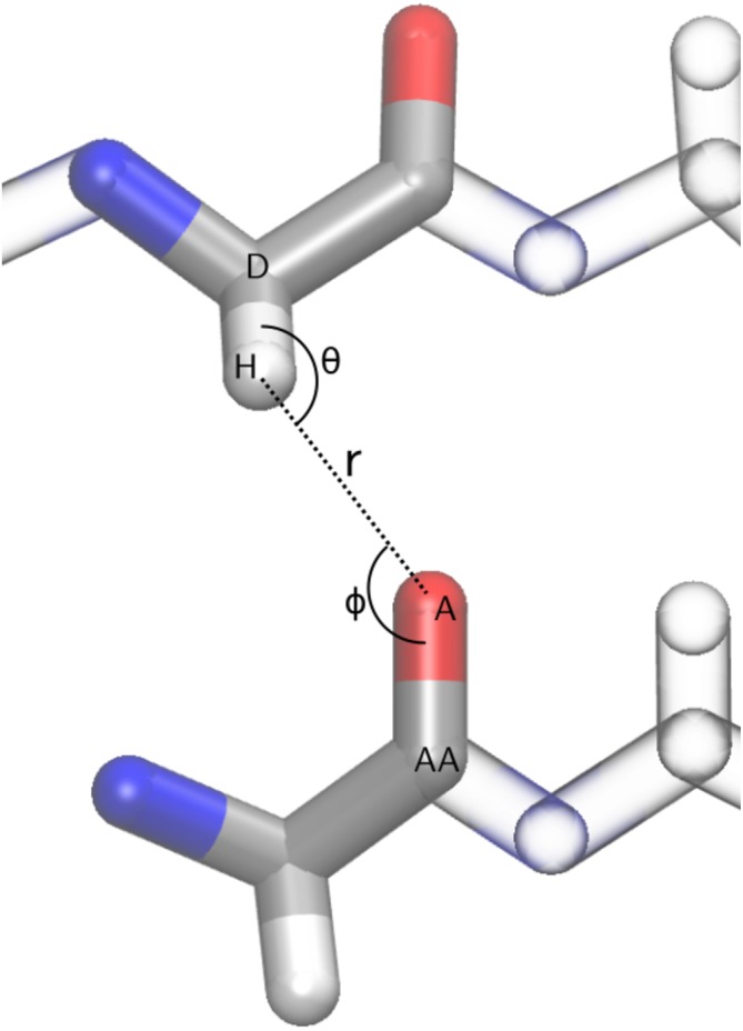
Definition of hydrogen bond geometry with the abbreviations D for donor atom, H for proton, A for acceptor, and AA for acceptor antecedent

Table 1.

Seven classes of hydrogen bonds

Class	Acceptor	Protona	Sizeb
I	Backbone O	HN, Δn = 4	961,238
II	Backbone O	HN, Δn ≠ 4	698,464
III	Backbone O	Sidechain proton	371,138
IV	Hydroxl Oc	Any proton	208,852
V	Carboxylic acid Od	Any proton	479,832
VI	Sidechain carbonyl Oe	Any proton	152,879
VII	Histidine N	Any proton	9,958

^aProton involved in hydrogen bond. Δn denotes residue separation.

^bNumber of database hydrogen bond geometries used to create surface.

^cFor serine, threonine, and tyrosine sidechain oxygens.

^dFor glutamic acid and aspartic acid sidechain oxygens.

^eFor glutamine and asparagine sidechain oxygens.

The surfaces were generated from coordinates taken from the Top8000 database16 of high‐resolution quality‐filtered protein crystal structures, a database used, for instance, in the calibration of the MolProbity17 package for protein structure validation. For each structure, the following process was performed:

• Missing protons were added with correct geometry using the Xplor‐NIH function protocol.addUnknownAtoms.

• For each acceptor and labile proton, a potential hydrogen bond was considered if the distance r between them was 3 Å or less.

• The putative hydrogen bond was excluded if:

  • any of the associated four atoms (donor, proton, acceptor, or acceptor antecedent) was involved in a steric clash, as reported by the RepelPot.bumps function;
  • any of the atoms had a B‐factor greater than 35 Ų.

• Parameters r, θ, and ϕ of the remaining hydrogen bonds were collected.

The number of hydrogen bond geometries included for generating each surface is shown in Table 1.

Once the parameters were collected a smooth probability distribution P(r,θ,ϕ) was generated for each class using adaptive kernel density estimation (KDE)18 with the Xplor‐NIH module densityEstimation initially developed for the TorsionDB energy term,19 using a Gaussian kernel and an overall window width of 0.2. This distribution was evaluated on a grid with spacing of 3° in the angular degrees of freedom and 0.072 Å in r. Using P(r,θ,ϕ), a potential of mean force can immediately be defined as

$$E_{\text{HBPot}}^0\left(r,\theta ,\varphi \right)=-\ln P\left(r,\theta ,\varphi \right),$$ (2)

where $E_{\text{HBPot}}^0$ was computed on the 3D grid, and rendered a continuous function of its variables using cubic interpolation.

We desire a smooth, attractive hydrogen bonding term which can be evaluated at all values of r but goes to zero for large r. As written in Equation (2), $E_{\text{HBPot}}^0\left(r,\theta ,\varphi \right)$ does not have this latter property, but rather gets larger as r increases. There is no such issue in the θ and ϕ degrees of freedom. To allow a gradual cutoff at large r, the following formula was used to define an energy term smooth in r which goes to zero at large values:

$$\begin{array}{c}{E}_{\text{HBPot}}\left(r,\theta ,\varphi \right)=w_{\text{HBPot}}\mathrm{Sw}\left(r\right)\times \\ \frac{E_{\text{HBPot}}^0\left(r,\theta ,\varphi \right)-\max E_{\text{HBPot}}^0\left(r_{\mathrm{off}},\cdot ,\cdot \right)}{\max E_{\text{HBPot}}^0\left(r_{\mathrm{off}},\cdot ,\cdot \right)-\min E_{\text{HBPot}}^0\left(\cdot ,\cdot ,\cdot \right)},\end{array}$$ (3)

where $\max E_{\text{HBPot}}^0\left(r_{\mathrm{off}},\cdot ,\cdot \right)$ denotes the maximum value of $E_{\text{HBPot}}^0$ on the two‐dimensional (2D) surface r = r_off and $\min E_{\text{HBPot}}^0\left(\cdot ,\cdot ,\cdot \right)$ is the minimum overall value of $E_{\text{HBPot}}^0$. Sw(r) is a piecewise continuous switching function:

$$\mathrm{Sw}\left(r\right)=\left\{\begin{array}{ll}1& r<r_{\mathrm{on}},\\ \frac{\left({r^2-r_{\mathrm{off}}^2)}^2\right(r_{\mathrm{off}}^2+2r^2-3r_{\mathrm{on}}^2)}{{(r_{\mathrm{off}}^2-r_{\mathrm{on}}^2)}^3}& r_{\mathrm{on}}<r<r_{\mathrm{off}},\\ 0& r>r_{\mathrm{off}}.\end{array}\right.$$ (4)

We use values of 3 and 4 Å for r_on and r_off, respectively. Thus, the minimum value of E_HBPot is −w_HBPot and it goes smoothly to zero at r = r_off.

2.1. Example HBPot surfaces

Example isoenergetic surfaces (isosurfaces) associated with the HBPot term are depicted in Figures 2, 3, 4 with the energy scale w_HBPot = 1. Figure 2 depicts 3D isosurfaces for the Class V term (involving glutamic/aspartic acid sidechain oxygens). Two local minima with distinct values of r and θ are evident at lower energies. Reassuringly, the surfaces are rather smooth. Figure 3 shows 2D cross‐sections through the Class VI surface (involving glutamine/asparagine sidechain oxygens) at three values of constant r. Also shown in this figure are the input data points used to generate the surface. The appearance of two minima at r = 3 Å is consistent with the qualitative distribution of points. In Figure 4, energy isosurfaces of constant ϕ are depicted for Class I, II, and VI, along with input points used to generate them. The dashed curve in this figure represents the empirical HBDA relationship between r and θ, which is seen to approximately follow the trough of minimal HBPot energy as one moves from the energy minimum to larger values of r and θ. It is noteworthy that the surfaces for the different classes are rather distinct, with the locations of the minima displaced relative to one another, and the relative location of the HBDA curve switching from one side of the trough to the other.

Figure 2.

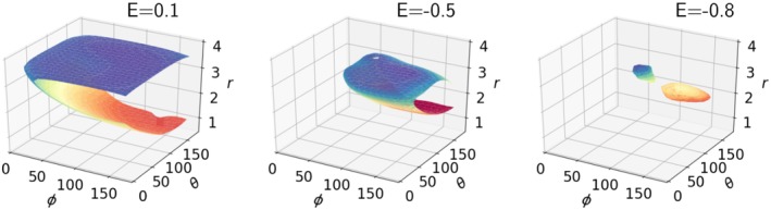
Surfaces of constant HBPot energy for the Class V hydrogen bonds (involving glutamic acid and aspartic acid sidechain oxygens) at three different values of energy for w_HBPot = 1. Units for r are Å, while θ and ϕ are in degrees

Figure 3.

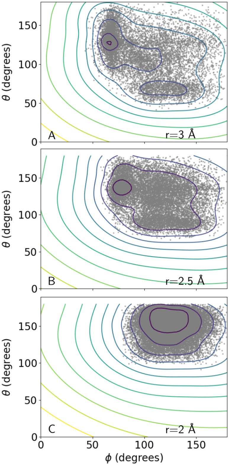
Panels (a)–(c) depict isosurfaces of 2D cross‐sections of the Class VI HBPot energy surface (involving glutamine and asparagine sidechain oxygens) at three values of r. Each gray dot corresponds to an input data point from the Top8000 database within the indicated value of r ± 0.1 Å. Contours are drawn at energy intervals of 0.1, with the maximum contour plotted for an energy of 0.2, such that the minimum energy contours are drawn for values of −0.7, −0.7, and −0.9 in (a), (b), and (c), respectively

Figure 4.

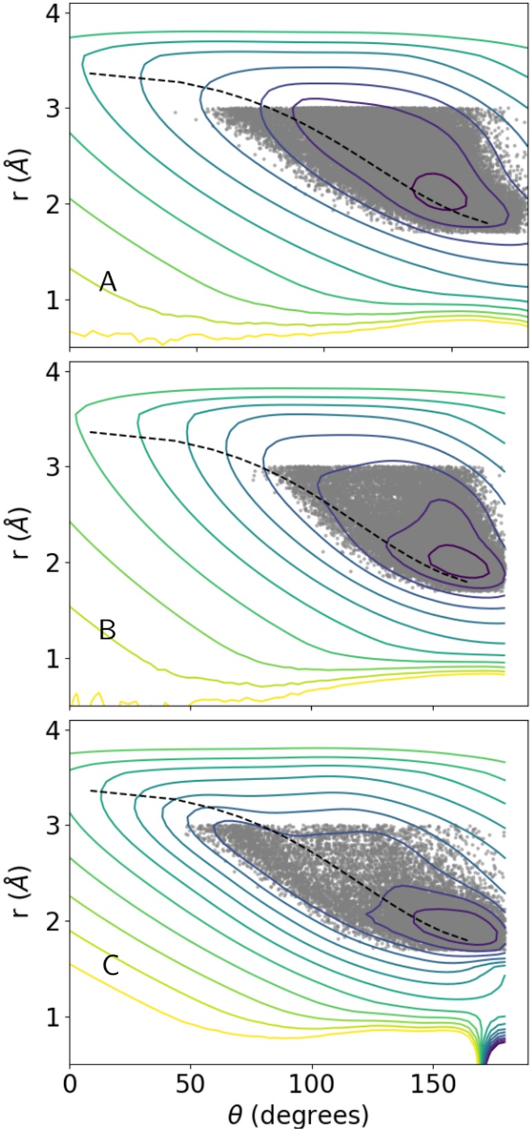
2D contour plots of constant density through the 3D HBPot surfaces at ϕ = 130°. Panels (a)–(c) depict the Class I helix backbone–backbone, Class II non‐helix backbone–backbone, and Class VI sidechain glutamine/asparagine surfaces, respectively. The dashed curve corresponds to Equation (1), the HBDA target relationship between r and θ. Each gray dot corresponds to an instance of hydrogen bonding geometry from the Top8000 database if the corresponding value of ϕ has a value of 130 ± 4°. Contours are drawn at energy intervals of 0.1 with the maximum contour plotted for an energy of 0.2, such that the minimum energy contours are drawn for −0.7, −0.8, and −0.9 in panels (a), (b), and (c), respectively

3. APPLICATION OF THE HBPOT TERM TO REFINEMENT OF 10 EXAMPLE PROTEINS

To evaluate the effects of HBPot on protein structure calculation, the term was tested on 10 protein systems used in a previous study,19 that range from 56 to 259 residues in length. These proteins and associated restraints used for structure determination are described in table II of Reference 19. In that publication, structure determination followed a two‐step procedure in which the proteins were initially folded using experimental distance and dihedral restraints, and the resulting lowest energy structure refined with additional energy terms. Here, we start with coordinates of the lowest energy structure from that previous fold step and apply the refinement protocol described below, examining the effect of adding HBPot, and then comparing this with results obtained using the HBDB term.

The refinement protocol is loosely based on that described in detail in Reference 5. First, covalent violations are removed in the starting structure using the function protocol.fixupCovalentGeom. Subsequently, high‐temperature MD is run at 3,000 K for 10,000 steps or 20 ps, whichever comes first. The simulated annealing schedule follows, consisting of MD runs for the shorter of 200 steps or 0.4 ps from temperatures of 3,000 K to 25 K at intervals of 12.5 K. Uniform atomic masses of 100 Da were used throughout. For each example, 100 structures were thus calculated differing in the random velocities chosen at the beginning of high‐temperature MD; the lowest energy 20 structures were then used for analysis.

For each example protein, the experimental restraints comprised interatomic distance information (including explicit hydrogen bonded pairs), dihedral restraints and residual dipolar couplings (RDCs). The distance restraints were applied with an energy scale of 2 during high‐temperature MD, and geometrically ramped from 2 to 30 during simulated annealing. The dihedral restraints were included with an energy scale of 10 during high‐temperature MD, and a constant energy scale of 200 during simulated annealing. The alignment tensor used in the back‐calculation of RDCs from structure was allowed to fully float during MD calculations, and during simulated annealing the optimal value was recalculated at each simulated annealing temperature before the next round of MD. The RDC energy scale was geometrically ramped from 0.05 to 5 during simulated annealing, with the initial value also used during high‐temperature MD.

The nonexperimental energy terms that comprise the default Xplor‐NIH force field include covalent bond length, bond angle, and improper dihedral terms, TorsionDB19 to bias proper rotatable dihedral angles toward populated regions of Ramachandran and sidechain space, and the purely repulsive RepelPot term8 to prevent atomic overlap. A constant energy scale of 1 was used for the bond length term throughout structure calculations, while that on the bond angle and improper terms was geometrically ramped from 0.4 to 1 and 0.1 to 1, respectively, during simulated annealing. The energy scale applied to the TorsionDB term was ramped from 0.002 to 2 and that on the RepelPot term from 0.004 to 4. During high‐temperature MD the initial energy scale values were used for each term and RepelPot interactions were only considered between Cα atoms. The HBDB hydrogen bonding term was enabled by adding the Xplor‐NIH snippet in Listing 1, while that used to enable the new HBPot term is specified in Listing 2. The energy scale factor w_HBPot was set to 2.5 kcal/mol when this term was enabled.

protocol.initHBDB()

potList.append(XplorPot('HBDB'))

Listing 1: Xplor‐NIH script snippet to configure the HBDB term.

import hbPotTools

hbond = hbPotTools.create_HBPot('hbond')

hbond.setScale(2.5)

potList.append(hbond)

Listing 2: Xplor‐NIH script snippet to configure the new HBPot term. Optional arguments to the create_HBPot function can be used to apply this term to a subset of atoms, to specify alternate energy surfaces, or to alter the energy threshold used to compute “violated” hydrogen bonds.

3.1. Results of structure refinement calculations

We evaluated the effect that the addition of HBPot has on the agreement of the other restraints used in the refinement calculation. We first examined the default nonexperimental restraints which are normally used in all protein structure calculations and which comprise the default Xplor‐NIH force field. In Figure 5, results are presented for each protein for three refinement calculations: one with no hydrogen bonding energy term, one using HBDB, and one with the new HBPot. In Figure 5a–c, one can see that the effect of adding either hydrogen bonding term is rather small on, respectively, the bond length, bond angle, and improper dihedral‐angle restraints. While the number of terms which are significantly violated (bond violated by more than 0.05 Å, or angle violated by more than 2°) is unchanged using either term (not shown), there is a definite trend that indicates the use of HBDB results is a slight decrease in angle and improper RMSD relative to the other cases. This is likely due to the fact that the coordinates used to describe HBDB geometry include these degrees of freedom around the carbonyl carbon through the use of a local Cartesian coordinate system based on this atom for HBDB's 3D surface. It appears that these angle and improper terms are double‐counted when the HBDB term is used, effectively increasing the energy scale on a subset of angles and impropers. On the other hand, the coordinate system used by HBPot (Figure 1) does not directly involve any local covalent geometry such that its effect on the angle and improper RMSD is negligible.

Figure 5.

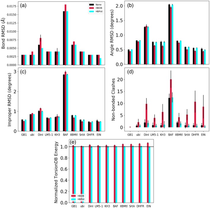
The effect of the hydrogen bonding energy terms on the nonexperimental covalent, nonbonded, and dihedral‐angle terms. Black bars report values for the case of no explicit hydrogen bonding term, while red and cyan report results for the HBDB and HBPot terms, respectively. Panels (a), (b), and (c) depict root mean square deviation from ideal values of the bond, bond angle, and improper dihedral‐angle covalent energy terms. Panel (d) depicts the number of nonbonded clashes, as reported by Xplor‐NIH. Panel (e) reports the TorsionDB potential of mean force energy including an explicit hydrogen bonding term normalized by the TorsionDB energy observed when no hydrogen bonding term is used. In each panel, a smaller value indicates structures which are more consistent with the Xplor‐NIH force field, and the spread in value among the 20 lowest energy structures is indicated by the thin black error bars

Figure 5d depicts the number of nonbonded violations (occurring when atoms are closer by 0.2 Å than the sum of their scaled van der Waals radii) as reported by Xplor‐NIH. Here we see that the addition of the HBDB term significantly increases the number of atomic clashes relative to the use of HBPot or of calculations using no hydrogen bonding term.

The TorsionDB term 19 comprises the dihedral‐angle portion of the default Xplor‐NIH force field. Because the energy is system‐size dependent, we choose to present the ratio of this term's energy with the two hydrogen bonding terms relative to the energy with no such term in Figure 5e. For all proteins one sees that the use of HBDB increases the TorsionDB energy, while using HBPot consistently has little effect. HBDB was developed without the use of an independent dihedral energy term, and found to improve dihedral‐angle geometries relative to calculations without HBDB.12 The calculations here, however, do include a dihedral‐angle term (TorsionDB), a term that is seen to be somewhat inconsistent with HBDB.

The effect of adding a hydrogen bonding term on the fit experimentally determined restraints is shown in Figure 6a–c for distance, dihedral‐angle and RDC restraints. Across all the test cases the HBDB term worsens the fit of the back‐calculated observables to those determined experimentally, while the HBPot term has little effect on the fit within the scatter of the calculated structures. Figure 6d depicts the RDC R‐factor for an alternate calculation in which the RDC term was omitted from the energy function. In this case, the differences in RDC fit are generally within the spread of the calculation, suggesting that structural accuracy is not significantly affected.

Figure 6.

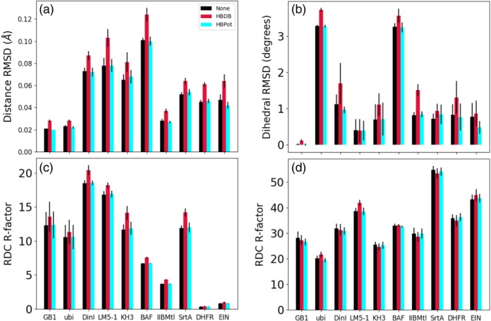
The effect of the hydrogen bonding energy terms on the agreement of experimental restraints with back‐calculated values for 10 proteins. Panels (a) and (b) depict root mean square deviation agreement for distance and dihedral restraints, respectively. Agreement of RDC data calculated from structures is shown in panels (c) and (d). Panel (c) shows the RDC R‐factor for the calculation with the RDC term included in the structure calculation, while Panel (d) shows the R‐factor for calculations run without this term. In all panels, a smaller value indicates better agreement with experiment, and the spread in value among the 20 lowest energy structures is indicated by the thin black error bars

To compare changes in the structures associated with using these different hydrogen bonding terms, for each example, mean structures were computed by averaging over the lowest energy 20 structures, and then regularized by applying gradient minimization under the respective, full final set of energy terms and energy scale factors. The mean square deviation in backbone (N, Cα, C′, and O atoms) coordinate position between these regularized average structures is illustrated in Figure 7. Disordered residues were excluded from the fit; the specific regions used for each case were ubi: residues 1–71, KH3: residues 13–25, 27–30, 33–52, 57–81, LM5‐1: residues 20–78, IIBMtl: residues 11–107, SrtA: residues 1–148, DHFR: residues 1–12, 37–161, EIN: residues 1–232, and all residues for proteins not listed. In all the examples but one, the differences between the structures calculated using HBDB and those calculated with no explicit hydrogen bonding term are significantly larger than those between the structures calculated using HBPot and no term, and similar to the differences in structures computed with the two different hydrogen bonding terms. This behavior dovetails with results from Figures 5 and 6, indicating that the use of HBPot represents a smaller, more consistent perturbation to the calculations than does HBDB. For sidechain atoms the pattern of agreement is similar, but with larger values (not shown).

Figure 7.

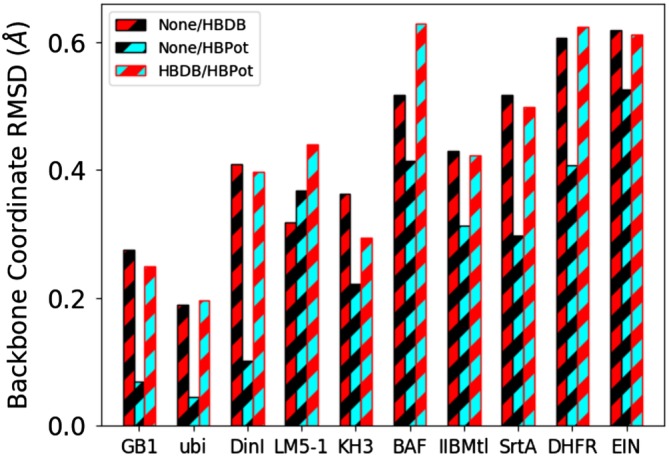
Backbone positional RMSD between regularized mean structures calculated with no hydrogen bonding term, using the HBDB term, and using the HBPot term for 10 proteins. The black/red bars represent the difference between structures computed with no hydrogen bonding term and those computed including the HBDB term. The black/cyan bars represent the differences between structures computed with no hydrogen bonding term with those computed including the HBPot term. The red/cyan bars represent the differences between structures calculated including HBDB or HBPot terms

Reference crystal structures exist for four of the systems studied here, and root mean square deviations in the fit coordinates of the calculated structures to the respective crystal structures are shown in Figure 8 for both backbone (panel a) and sidechain (panel b) atomic coordinates. Here, we see that the inclusion of a hydrogen bonding term leads to small improvements in accuracy, with the use of HBPot leading to slightly more accurate structures in all but one case. However, these improvements are generally within the spread of the calculated structures. Because these examples include curated restraints, they are expected to already be rather accurate. The RDC restraints themselves strongly restrain backbone coordinates, such that the hydrogen bonding terms act as small perturbations. And while it is expected that adding the HBPot term would improve sidechain accuracy, this is a localized improvement which is apparently largely obscured by structural noise of the calculation in the RMSD metric.

Figure 8.

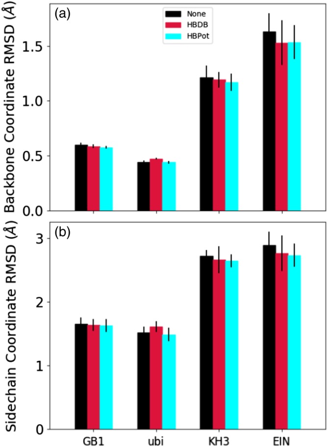
Positional RMSD between structures calculated from NMR data compared with the corresponding crystal structures for GB1, ubiquitin, KH3, and EIN. Spread in fit among the 20 lowest energy structures is indicated by the thin black error bars. Panel (a) depicts the backbone atomic accuracy, while Panel (b) shows the sidechain accuracy measured after fitting backbone atomic coordinates

Figure 9 depicts the number of hydrogen bonds as reported by the HBDB and HBPot terms and by the program VMD.20 With the default configuration in Listing 1, HBDB reports as backbone–backbone hydrogen bonds, instances where the O–H distance is less than 2.6 Å, both the θ and C–O–H angles are less than 100°, and the donor and acceptor are at least three residues apart. To count hydrogen bonds with the VMD we used the commonly used command:

Figure 9.

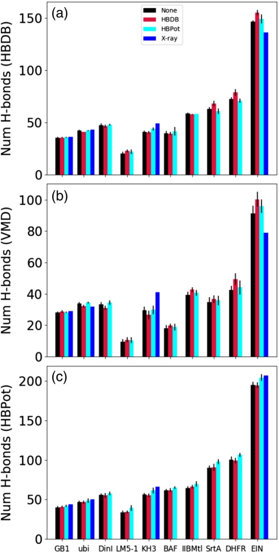
The number of hydrogen bonds reported by HBDB, VMD, and HBPot are shown in panels (a), (b), and (c), respectively, for the cases of no explicit hydrogen bond term, the use of the HBDB term, and the use of the HBPot term. The VMD and HBDB numbers report only on number of backbone–backbone hydrogen bonds. The blue bars represent the number of hydrogen bonds measured from the protonated reference structures for the four examples for which there are crystal structures

measure hbonds 3.5 30 \

[atomselect top "protein and name N"]\

[atomselect top "protein and name O"]

which selects all pairs of backbone donor and acceptor atoms separated by less than 3.5 Å with a θ angle of less than 150°. HBPot simply reports a hydrogen bond as any donor and acceptor separated by at least four amino acids and where the proton‐acceptor distance is less than 4 Å; any angular dependence on geometry is handled by the potential of mean force. Because HBDB has a more generous angular threshold than that used with VMD, the numbers are larger in Figure 9a than in 9b, and because HBPot contains no angular criteria, has a much larger distance cutoff, and includes backbone–sidechain and sidechain–sidechain hydrogen bonds in addition to backbone–backbone hydrogen bonds, the numbers it reports are much larger. In Figure 9c, it is seen that the use of HBPot consistently, if modestly, increases the number of hydrogen bonds as it defines them, as expected. This figure also shows that use of HBDB does not increase the number of hydrogen bonds as defined by HBPot. Panels (a) and (b) of this figure show that using HBDB increases the respective hydrogen bond count for four and six proteins, respectively. Interestingly, the use of HBDB leads to a decrease in the number of hydrogen bonds in two cases in Figure 9a and three cases in Figure 9b.

For the four examples which have corresponding crystal structures, blue bars in Figure 9 represent the number of hydrogen bonds in these structures (with protons added). For most cases, the numbers of hydrogen bonds are larger for the crystal structures than those calculated from nuclear magnetic resonsance (NMR) data, regardless of the method of counting. This observation is consistent with the understanding that high‐resolution crystal structures are generally more accurate than NMR structures, and would thus have more hydrogen bonds. For EIN, only when using the relaxed definition of hydrogen bond of HBPot does the crystal structure have a larger hydrogen bond count. This result suggests that the crystal structure of EIN has many hydrogen bonds with unusual geometry which may indicate a lower quality structure. It should be noted that only the relaxed HBPot method of counting hydrogen bonds consistently gives the largest number for crystal structures.

While Figure 9 reports on the number of hydrogen bonds, the quality of hydrogen bonding can be better inferred from the associated energy. In Figure 10, Xplor‐NIH hydrogen bonding energies for the HBDA, HBDB and HBPot terms are reported divided by their values computed when no hydrogen bonding term was included. Histogram bars which lie below the horizontal black lines represent cases where the use of the respective HBDB or HBPot term lowers the reported energy, indicating improved fit, while bars above the line indicate higher energy/worse fit. Figure 10a indicates that using HBDB generally worsens the agreement to the HBDA relationship in Equation (1), while HBPot improves the fit for nine of the 10 examples. Figure 10c shows that use of HBPot consistently lowers the associated energy, as expected, but use of the HBDB term does not lower this energy. Figure 10b shows that use of HBPot consistently lowers the HBDB energy—more consistently than use of the HBDB term itself which results in significantly higher energies in three cases. This surprising pathological behavior of the HBDB term probably indicates the presence of local minima at higher energies which are selected in our refinement procedure.

Figure 10.

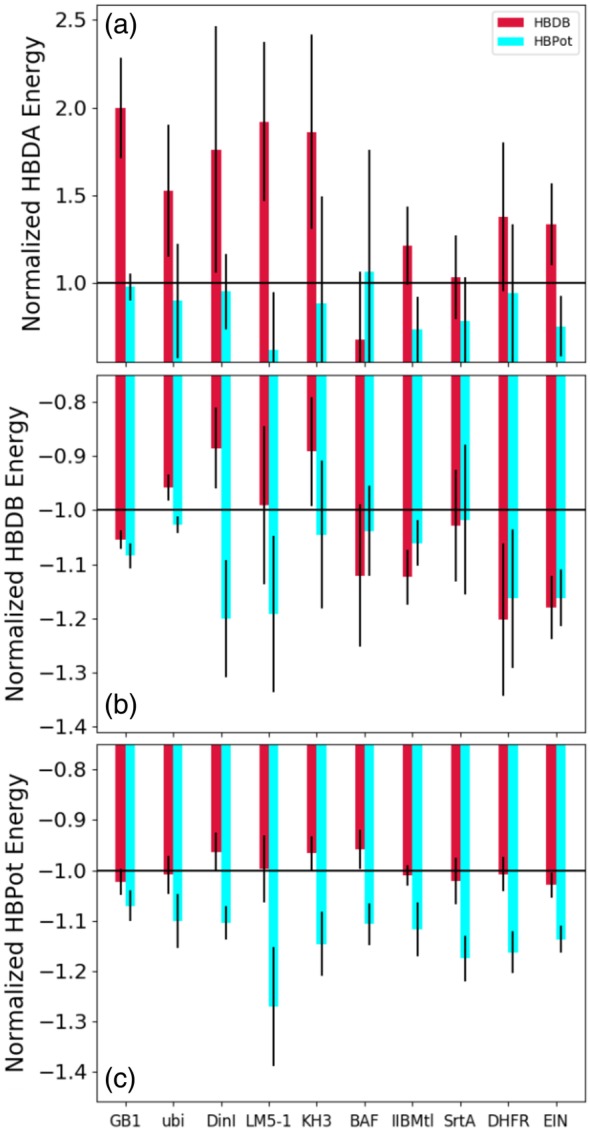
Hydrogen bond energies report the efficacy of the hydrogen bond energy terms. Panels (a), (b), and (c) report the HBDB, HBPot, and HBDA energy terms for the 10 protein example cases with either the HBDB or HBPot energy term, normalized by the energy corresponding to the calculations with no explicit hydrogen bonding energy. In each panel a horizontal line indicates signed unity, the normalized energy corresponding to using no hydrogen bonding term. Because a smaller (more negative or less positive) value indicates a better fit to the potential of mean force or (in the case of HBDA) empirical formula, bars below/above the line represent better/worse fits for the depicted energy term. For each bar, deviations in energy between the lowest 20 calculated structures are denoted by the thin black error bars

4. CONCLUSION

We have introduced a new hydrogen bonding potential of mean force that biases hydrogen bond geometries toward those observed in high‐resolution crystal structures in the PDB. In comparison with the currently used hydrogen bonding potential, HBDB, we have shown that this new term is much more consistent with the default Xplor‐NIH force field, and with NMR‐derived experimental restraints. As generation of this new term utilized the well‐developed algorithms of adaptive KDE to produce smooth surfaces, and care was taken to smoothly switch the energy to zero at large proton‐acceptor distance, pathological artifacts of the type displayed by the HBDB term have not been observed in structure calculations. Because HBPot was developed in the modern Xplor‐NIH Python/C++ environment, it can be used to influence inter‐subunit hydrogen bonds when using the symSimulation strict symmetry facility. Thread‐level parallelization is straightforward using OpenMP directives. HBPot contains less explicit dependence on local secondary structure than HBDB so it follows that the new term should have less tendency to force regular structure on regions where there is none. Finally, unlike HBDB, HBPot includes hydrogen bonds involving protein sidechain atoms.

HBPot has been shown to improve hydrogen bonding geometry and be preferable to the older HBDB term in refinement calculations including RDCs. Further work is necessary to demonstrate an improvement in coordinate accuracy when less complete NMR data sets or erroneous restraints are utilized in structure calculation. However, given the current results, we expect that the addition of HBPot will not significantly distort structures calculated from NMR data, while it should increase the number of hydrogen bonds.

Further work is necessary to determine the usefulness of these PDB‐derived potentials of mean force to nonprotein structure calculations, for instance, to those involving nucleic acids or nucleic acid–protein complexes. Preliminary calculations of RNA structures with HBPot indicate that the application of this term does not interfere with structure calculation, but there is also little indication that it improves these structures. However, it should be noted that RNA has hydrogen bonding classes not included in Table 1, such as those involving the phosphorous‐bonded oxygen or the ribose ether oxygen acceptors, so it is likely necessary to generate new energy surfaces for these classes from a library of high‐quality RNA crystal structures. Moreover, RNA hydrogen bonding is dominated by base pairing, which is already highly restrained in standard Xplor‐NIH calculations by distance and planarity restraints, and by the ORIE21, 22 base packing potential of mean force. Non‐base‐pair hydrogen bonds should be more important for RNAs with noncanonical structure and protein‐RNA complexes.

CONFLICT OF INTEREST

The authors declare no conflict of interest.

Schwieters CD, Bermejo GA, Clore GM. A three‐dimensional potential of mean force to improve backbone and sidechain hydrogen bond geometry in Xplor‐NIH protein structure determination. Protein Science. 2020;29:100–110. 10.1002/pro.3745

REFERENCES

- 1. Latimer WM, Rodebush WH. Polarity and ionization from the standpoint of the Lewis theory of valence. J Am Chem Soc. 1920;42:1419–1433. [Google Scholar]
- 2. Mirsky AE, Pauling L. On the structure of native, denatured, and coagulated proteins. Proc Natl Acad Sci U S A. 1936;22:439–447. [DOI] [PMC free article] [PubMed] [Google Scholar]
- 3. Pace CN, Hailong F, Fryar KL, et al. Contribution of hydrogen bonds to protein stability. Protein Sci. 2014;23:652–661. [DOI] [PMC free article] [PubMed] [Google Scholar]
- 4. Brooks BR, Brooks CL III, Mackerell AD Jr, et al. CHARMM: The biomolecular simulation program. J Comput Chem. 2009;30:1545–1614. [DOI] [PMC free article] [PubMed] [Google Scholar]
- 5. Bermejo GA, Schwieters CD. Protein structure elucidation from NMR data with the program Xplor‐NIH. Methods Mol Biol. 2018;1688:311–340. [DOI] [PMC free article] [PubMed] [Google Scholar]
- 6. Schwieters CD, Kuszewski JJ, Tjandra N, Clore GM. The Xplor‐NIH NMR molecular structure determination package. J Magn Reson. 2003;160:65–73. [DOI] [PubMed] [Google Scholar]
- 7. Schwieters CD, Kuszewski JJ, Clore GM. Using Xplor‐NIH for NMR molecular structure determination. Progr NMR Spectroscopy. 2006;48:47–62. [Google Scholar]
- 8. Schwieters CD, Bermejo GA, Clore GM. Xplor‐NIH for molecular structure determination from NMR and other data sources. Protein Sci. 2018;27:26–40. [DOI] [PMC free article] [PubMed] [Google Scholar]
- 9. Brünger AT. XPLOR manual version 3.1. New Haven, CT: Yale University Press, 1993. [Google Scholar]
- 10. Bermejo GA, Clore GM, Schwieters CD. Improving NMR structures of RNA. Structure. 2016;24:806–815. [DOI] [PMC free article] [PubMed] [Google Scholar]
- 11. Lipsitz RS, Sharma Y, Brooks BR, Tjandra N. Hydrogen bonding in high‐resolution protein structures: A new method to assess NMR protein geometry. J Am Chem Soc. 2002;124:10621–10626. [DOI] [PubMed] [Google Scholar]
- 12. Grishaev A, Bax A. An empirical backbone‐backbone potential in proteins and its application to NMR structure refinement and validation. J Am Chem Soc. 2004;126:7281–7292. [DOI] [PubMed] [Google Scholar]
- 13. Morozov AV, Kortemme T, Tsemekhman K, Baker D. Close agreement between the orientation dependence of hydrogen bonds observed in protein structures and quantum mechanical calculations. Proc Natl Acad Sci U S A. 2004;101:6946–6951. [DOI] [PMC free article] [PubMed] [Google Scholar]
- 14. Rohl CA, Strauss CEM, Misura KMS, Baker D. Protein structure prediction using Rosetta. Meth Enz. 2004;383:66–93. [DOI] [PubMed] [Google Scholar]
- 15. Stickle DF, Presta LG, Dill KA, Rose GD. Hydrogen bonding in globular proteins. J Mol Biol. 1992;226:1143–1159. [DOI] [PubMed] [Google Scholar]
- 16.Available from: http://kinemage.biochem.duke.edu/databases/top8000.php.
- 17. Chen VB, Arendall WB III, Headd JJ, et al. MolProbity: All‐atom structure validation for macromolecular crystallography. Acta Crystallogr. 2010;D66:12–21. [DOI] [PMC free article] [PubMed] [Google Scholar]
- 18. Silverman BW. Density estimation for statistics and data analysis. London: Chapman and Hall, 1986. [Google Scholar]
- 19. Bermejo GA, Clore GM, Schwieters CD. Smooth statistical torsion angle potential derived from a large conformational database via adaptive kernel density estimation improves the quality of NMR protein structures. Protein Sci. 2012;21:1824–1836. [DOI] [PMC free article] [PubMed] [Google Scholar]
- 20. Humphrey W, Dalke A, Schulten K. VMD‐visual molecular dynamics. J Mol Graph. 1996;14:33–38. [DOI] [PubMed] [Google Scholar]
- 21. Kuszewski JJ, Schwieters CD, Clore GM. Improving the accuracy of NMR structures of DNA by means of a database potential of mean force describing base‐base positional interactions. J Am Chem Soc. 2001;123:3903–3918. [DOI] [PubMed] [Google Scholar]
- 22. Clore GM, Kuszewski JJ. Improving the accuracy of NMR structures of RNA by means of conformational database potentials of mean force as assessed by complete dipolar coupling cross‐validation. J Am Chem Soc. 2003;125:1518–1525. [DOI] [PubMed] [Google Scholar]