Optimal control of a discrete age-structured model for tuberculosis transmission

Abstract

In this present paper, a discrete age-structured model of tuberculosis (TB) transmission is formulated and analyzed. The existence and stability of the model equilibriums are discussed based on the basic reproduction ratio. A sensitivity analysis of the model parameters is determined. We then apply the optimal control strategy for controlling the transmission of TB in child and adult populations. The control variables are TB prevention, chemoprophylaxis of latent TB, and active TB treatment efforts. The optimal controls are then derived analytically using the Pontryagin Maximum Principle. Various intervention strategies are performed numerically to investigate the impact of the interventions. We used the incremental cost-effectiveness ratios (ICER) to assess the benefit of each one the control strategies.

Applied mathematics; Computational mathematics; Epidemiology; Systems biology; Systems theory; Tuberculosis; Discrete age-structured model; Stability; Basic reproduction ratio; Optimal control

1. Introduction

Tuberculosis (TB) is an airborne infectious disease. It is caused by the bacillus Mycobacterium tuberculosis. TB is a major global health problem, and the mortality rate without treatment is high; in fact, TB is one of the top ten diseases causing high mortality. Researchers have found that 70% of people with sputum smear-positive pulmonary TB die within ten years [1]. Based on that prevalence, there were 1.4 million TB deaths and 10.4 million new TB cases, including 5.9 million new cases in men, 3.5 million in women, and 1.0 million in children. The data include 1.2 million HIV-positive patients [1]. About one-third of the world's population has latent TB infections. People with latent TB infections have been infected by the TB bacteria, but they are not infectious [2].

TB attacks both children and adults. Children with latent TB infections are difficult to diagnose. The symptoms of a TB infection in a child only emerge when they have a cough and fever, in some cases it is tied in with influenza. There is little transmission risk, from children with TB. Hence, TB affecting various age groups can indicate a new transmission method [3]. One million children under 14 years have been infected with TB, and 170,000 TB-infected children (excluding children with HIV coinfection) died from the disease in 2015 [2].

Mathematical models have become effective tools with which to understand the dynamics of TB transmission. Some deterministic and stochastic models for TB have been developed to address the spread of the disease, see, for instance, [4], [5]. The model in [4] discussed the dynamics of a TB outbreak by considering the TB treatment effect at home. The stochastic model for a TB outbreak was shown in [5]. Furthermore, mathematical models of a dynamic TB outbreak with optimal control were presented in [6], [7], [8], [9], [10]. The TB model in [6] considered the optimal control for undetected TB cases. The authors in [7] analyzed the optimal strategy to a TB outbreak model by considering the migration of susceptible populations in each area. Silva and Torres discussed an optimal strategy for the TB model with reinfection and post-exposure interventions [8]. The authors in [9] studied optimal control interventions to minimize the number of infectious and latent TB populations using real data from Angola. Rodrigues et al. [10] applied an optimal control problem for TB model with exogenous reinfection. The cost-effectiveness analysis also was done in [10] to investigate the effect of each one of the control strategies, separately or combined.

A number of discrete age-structured mathematical models have been developed for vector-borne diseases such as in [11], [12], [13], [14]. For the epidemic models with direct transmission, most of the age-structured models is formulated in the form of integro-partial differential equations, such as in the TB model [15], [16], HIV model [17], and Buruli ulcer model [18]. Few studies have considered the discrete age-structure of an epidemic model with direct transmission. The authors in [19] investigated an epidemic model as an age-structured TB transmission model in discrete time units and applied it to predict TB infection in China.

In this present paper, we study the dynamics of a TB outbreak within a discrete age-structured population using ordinary differential system. We also explore the impact of the optimal control strategy in reducing latent and active TB populations. The controls are represented by TB prevention, chemoprophylaxis for latent TB, and treatment efforts. The main purpose of optimal control is to reduce latent and active TB populations. The remaining part of the paper is arranged as follows: the formulation of the TB model is addressed in Section 2. The stability analysis and sensitivity analysis of the model parameters are given in Sections 3 and 4. The application of the optimal control problem and the numerical simulation to support the analytic results are shown in Section 5 and 6. The cost-effectiveness discussion is performed in Section 7. The concluding remark is summarized in Section 8.

2. Model formulation

First, we construct a TB spread model by taking into account a single age-structured population. The population is assumed to be closed and is divided into four classes, which are the susceptible class (S), the latent TB class (E), the active TB class (I), and the recovered class (R). The latent TB class consists of hosts infected by TB bacteria, but without an infectious status. The active TB class consists of hosts with infectious status. The single age-structured TB spread model is as follows.

$$\frac{dS}{dt}=\mathrm{\Lambda }+\theta R-\beta SI-\mu S,\frac{dE}{dt}=\beta SI-(\alpha +\mu )E,\frac{dI}{dt}=\alpha E-(\gamma +\mu +d)I,\frac{dR}{dt}=\gamma I-(\mu +\theta )R.$$ (1)

We assume that the parameters used in the model equation (1) are constant and non-negative. Moreover, Table 1 consists of the interpretation of the parameters.

Table 1.

Parameters interpretation of the model (1).

Parameter	Interpretation
Λ	recruitment rate
θ	immunity loss rate
β	successful infection rate
μ	natural death rate
α	TB progression rate
γ	recovery rate
d	TB-induced death rate

Next, we construct a TB spread model by taking into account a discrete age-structured population. This model represents an extension of model (1). We split the population into child (C) and adult (A) populations. Furthermore, each population is partitioned into four classes, namely, the susceptible classes ($S_C$, $S_A$), the latent TB classes ($E_C$, $E_A$), the active TB classes ($I_C$, $I_A$), and the recovered classes ($R_C$, $R_A$). Therefore, the total size the population is $N=S_C+S_A+E_C+E_A+I_C+I_A+R_C+R_A$. In this second model, we use the average natural death rate of the total population, i.e., the natural death rates of the child and adult populations are assumed to be equal.

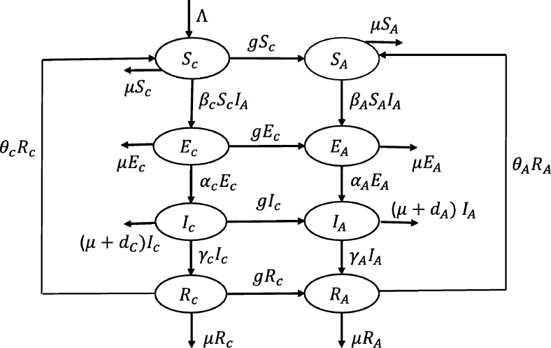
Children with TB are less likely to spread the TB bacteria to others [3], [20]. Hence, we assume that the children were infected by TB through contacts with active-TB adults. Hence, only the active TB adults can spread the TB bacteria in the population. The transmission diagram is given in Fig. 1 for deriving a discrete age-structured model. The model is derived as follows.

$$\frac{d{S}_C}{dt}=\mathrm{\Lambda }+{\theta }_C{R}_C-{\beta }_C{S}_C{I}_A-(\mu +g)S_C,\frac{d{S}_A}{dt}=g{S}_C+{\theta }_A{R}_A-{\beta }_A{S}_A{I}_A-\mu S_A,\frac{d{E}_C}{dt}={\beta }_C{S}_C{I}_A-({\alpha }_C+\mu +g)E_C,\frac{d{E}_A}{dt}={\beta }_A{S}_A{I}_A+g{E}_C-({\alpha }_A+\mu )E_A,\frac{d{I}_C}{dt}={\alpha }_C{E}_C-({\gamma }_C+\mu +g+d_C)I_C,\frac{d{I}_A}{dt}={\alpha }_A{E}_A+g{I}_C-({\gamma }_A+\mu +d_A)I_A,\frac{d{R}_C}{dt}={\gamma }_C{I}_C-(\mu +g+{\theta }_C)R_C,\frac{d{R}_A}{dt}={\gamma }_A{I}_A+g{R}_C-(\mu +{\theta }_A)R_A.$$ (2)

Figure 1.

A discrete age-structured TB transmission diagram.

All of the parameters used in model (2) are assumed to be constant and non-negative. Their description can be seen in Table 2. Furthermore, model (2) has the region of biological interest as follows.

$$\mathrm{\Omega }=\{(S_C,S_A,E_C,E_A,I_C,I_A,R_C,R_A)\in {\mathbb{R}}_{+}^8:0\le N\le \frac{\mathrm{\Lambda }}{\mu }\}.$$

Table 2.

Parameters description of model (2).

Description	Parameter
Recruitment rate into the population	Λ
Child survival rate	g
Natural death rate	μ
	Child	Adult
	population	population
Infection rate	βC	βA
Progression rate from latent to infectious	αC	αA
Natural recovery rate	γC	γA
Immunity loss rate	θC	θA
TB death rate	dC	dA

Model (2) is well-defined in the region Ω due to the vector field of the model on the boundary of the region Ω does not point to the exterior area. Hence, if we give an initial condition in the region, then the solution of the model is well-defined for all time $t\ge 0$ and remains in the feasible region Ω.

3. Analysis of the model

First, we analyze model (1). Model (1) has two equilibria. Its disease-free equilibrium is $E_0^s=(\frac{\mathrm{\Lambda }}{\mu },0,0,0)$ and its basic reproduction ratio is

$$R_0^s=\frac{\alpha \beta \mathrm{\Lambda }}{\mu (\alpha +\mu )(\gamma +\mu +d)}.$$ (3)

The basic reproduction ratio describes the expected number of secondary case from primary case during the infectious period of the primary case [21], [22].

Moreover, model (1) has the endemic equilibrium $E_1^s=(\frac{\mathrm{\Lambda }}{R_0^s\mu },E^s,I^s,R^s)$, where

$$E^s=\frac{(R_0^s-1)(\gamma +\mu +d)(\theta +\mu )\mathrm{\Lambda }}{R_0^s[(\theta +\mu )(d(\alpha +\mu )+\mu (\gamma +\mu ))+\alpha \mu (\gamma +\theta +\mu )]},I^s=\frac{(R_0^s-1)(\theta +\mu )\alpha \mathrm{\Lambda }}{R_0^s[(\theta +\mu )(d(\alpha +\mu )+\mu (\gamma +\mu ))+\alpha \mu (\gamma +\theta +\mu )]},R^s=\frac{(R_0^s-1)\alpha \gamma \mathrm{\Lambda }}{R_0^s[(\theta +\mu )(d(\alpha +\mu )+\mu (\gamma +\mu ))+\alpha \mu (\gamma +\theta +\mu )]}.$$

The equilibrium $E_0^s$ is locally asymptotically stable if $R_0^s<1$, otherwise it is unstable. Furthermore, the equilibrium $E_1^s$ exists and is locally asymptotically stable if $R_0^s>1$ [23].

Model (2) has disease-free equilibrium $E_0^t=(\frac{\mathrm{\Lambda }}{g+\mu },\frac{g\mathrm{\Lambda }}{\mu (g+\mu )},0,0,0,0,0,0)$. Furthermore, it has the basic reproduction ratio

$$R_0=\frac{g\mathrm{\Lambda }[{\alpha }_A{\beta }_A{\eta }_2{\eta }_4+{\beta }_C\mu ({\alpha }_A{\eta }_4+{\alpha }_C{\eta }_3)]}{\mu {\eta }_1{\eta }_2{\eta }_3{\eta }_4{\eta }_5},$$ (4)

where ${\eta }_1=g+\mu$, ${\eta }_2={\alpha }_C+\mu +g$, ${\eta }_3={\alpha }_A+\mu$, ${\eta }_4={\gamma }_C+\mu +g+d_C$ and ${\eta }_5={\gamma }_A+\mu +d_A$. The ratio $R_0$ comes from the $1\times 1$ next-generation matrix because only the active TB adult population $I_A$ can spread TB infections. Using Theorem 2 in [23], the equilibrium $E_0^t$ is locally asymptotically stable if $R_0<1$, otherwise it is unstable.

In addition to the equilibrium $E_0^t$, model (2) also has an endemic equilibrium $E_1^t=(S_C^t,S_A^t,E_C^t,E_A^t,I_C^t,I_A^t$, $R_C^t$, $R_A^t)$ if $R_0>1$. All of the components of $E_1^t$ are positive if $R_0>1$. The components depend on the equilibrium state $I_A^t$. The equilibrium state $I_A^t$ is the positive root of the quadratic equation $A{x}^2+Bx+C=0$, where

$$A={\beta }_A{\beta }_C({\eta }_3{\eta }_5{\eta }_7-{\alpha }_A{\gamma }_A{\theta }_A)({\eta }_2{\eta }_4{\eta }_6-{\alpha }_C{\gamma }_C{\theta }_C)>0,B={\eta }_1{\eta }_2{\eta }_4{\eta }_6{\beta }_A({\eta }_3{\eta }_5{\eta }_7-{\alpha }_A{\gamma }_A{\theta }_A)-g{\beta }_A{\beta }_C\mathrm{\Lambda }({\eta }_4{\eta }_6{\eta }_7{\alpha }_A+{\eta }_3{\eta }_6{\eta }_7{\alpha }_C+{\alpha }_A{\alpha }_C{\gamma }_C{\theta }_A)+{\eta }_3{\eta }_5{\eta }_7{\beta }_C\mu ({\eta }_2{\eta }_4{\eta }_6-{\alpha }_C{\gamma }_C{\theta }_C),C=-(R_0-1)\mu {\eta }_1{\eta }_2{\eta }_3{\eta }_4{\eta }_5{\eta }_6{\eta }_7,$$

where ${\eta }_6=\mu +g+{\theta }_C$ and ${\eta }_7=\mu +{\theta }_A$. The coefficient C has negative value if $R_0>1$. Hence, $I_A^t>0$ if $R_0>1$.

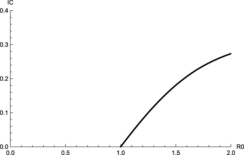
The equilibrium $E_1^t$ is locally asymptotically stable if $R_0>1$. The bifurcation diagram of model (2) with respect the ratio $R_0$ can be seen in Fig. 2.

Figure 2.

Bifurcation diagram of model (2).

4. Sensitivity analysis of parameters

In the present section, we implement a sensitivity analysis of the parameters from models (1) and (2). This allows us to determine the parameters that have a great influence on the basic reproduction ratios ($R_0^s$ and $R_0$). We adopt the same approach in [24] to derive the analytic formulation for the sensitivity index of $R_0^s$ and $R_0$ to each parameter. The sensitivity index of Q related to parameter k, is defined as

$${\mathrm{\Upsilon }}_k^Q:=\frac{\partial Q}{\partial k}\times \frac{k}{Q}.$$ (5)

The sensitivity indices ${\mathrm{\Upsilon }}_{\mathrm{\Lambda }}^{R_0^s}$, ${\mathrm{\Upsilon }}_{\beta }^{R_0^s}$, ${\mathrm{\Upsilon }}_{\mathrm{\Lambda }}^{R_0}$ are equal to one and do not depend on the values of the other parameters. The sensitivity indices of $R_0^s$ and $R_0$ related to the remaining parameters can be calculated in the same way as in (5). Using the parameter values in Table 3, their sensitivity indices are given in Table 4.

Table 3.

Parameter values for simulations.

Parameter	Value	Ref.	Parameter	Value	Ref.
Λ	1000	Assumed	γA	0.21	[34]
g	$\frac{1}{14}$	[2]	γC	0.2	[34]
β	0.02	[33]	θA	0.873	Assumed
βA	0.02	[33]	θC	0.83	Assumed
βC	0.01	[33]	μ	0.0143	[35]
α	0.005	[35]	d	0.05751	[36]
αA	0.005	[35]	dA	0.05751	[36]
αC	0.005	[35]	dC	0.0575	[36]
γ	0.21	[34]

Table 4.

Sensitivity index of the parameters in models (1) and (2).

Parameter (p)	Sensitivity index ${\mathrm{\Upsilon }}_p^{R_0^s}$	Parameter (p)	Sensitivity index ${\mathrm{\Upsilon }}_p^{R_0}$
Λ	1	Λ	1
β	1	g	0.000105
α	0.7409	βA	0.923
γ	-0.7452	βC	0.0768
μ	-1.7917	αA	0.7379
d	-0.2041	αC	-0.000143
		γA	-0.745
		γC	-0.00238
		μ	-1.89
		dA	-0.204
		dC	-0.000685

A positive index indicates that the value of $R_0^s$ or $R_0$ increases as a parameter is increased. To the contrary, a negative index means that the value of $R_0^s$ or $R_0$ decreases as a parameter is increased. The sensitivity index of ${\mathrm{\Upsilon }}_{{\beta }_A}^{R_0}=0.923$ means that an increase of 10% in the value ${\beta }_A$ will increase $R_0$ by 9.23%. Likewise, a sensitivity index of ${\mathrm{\Upsilon }}_{{\gamma }_A}^{R_0}=-0.745$ indicates that an increase of 10% in the value ${\gamma }_A$ will decrease $R_0$ by 7.45%.

Next, we compare the sensitivity indices of basic reproduction ratios of models (1) and (2) with respect to some parameters. From Table 4, it can be seen that, when using model (1), the sensitivity indices of the basic reproduction ratio $R_0^s$ with respect to the TB infection rate (β) and the TB progression rate (α) are 1 and 0.7409, respectively. While, for model (2), the sensitivity indices of the basic reproduction ratio $R_0$ with respect to the TB infection rates for adults (${\beta }_A$) and children (${\beta }_C$) are significantly different, i.e., 0.923 and 0.0768, respectively. Similarly, the sensitivity indices of the basic reproduction ratio $R_0$ with respect to TB progression for adults (${\alpha }_A$) and children (${\alpha }_C$) are 0.7379 and −0.000143, respectively. The significant difference in sensitivity indice values is due to the fact that only active TB adults can spread TB in the population. Hence, the discrete age-structured model provides a more realistic description of TB transmission in the population.

5. Formulation of the optimal control

In the present section, we propose the optimal control problem of the spread of TB within the discrete age-structured model. The control aspect to be optimized in this work is the prevention efforts ($u_1$) for the susceptible population, chemoprophylaxis ($u_2$) for the latent TB population, and treatment ($u_3$) for the active TB population. All of the controls are incorporated into the child and adult populations. The TB spread model involving the discrete age-structured population with three controls is as follows.

$$\frac{d{S}_C}{dt}=\mathrm{\Lambda }+{\theta }_C{R}_C-(1-u_1){\beta }_C{S}_C{I}_A-(\mu +g)S_C,\frac{d{S}_A}{dt}=g{S}_C+{\theta }_A{R}_A-(1-u_1){\beta }_A{S}_A{I}_A-\mu S_A,\frac{d{E}_C}{dt}=(1-u_1){\beta }_C{S}_C{I}_A-({\alpha }_c+\mu +g)E_C-{\delta }_C{u}_2{E}_C,\frac{E_A}{dt}=(1-u_1){\beta }_A{S}_A{I}_A+g{E}_C-({\alpha }_A+\mu )E_A-{\delta }_A{u}_2{E}_A,\frac{d{I}_C}{dt}={\alpha }_C{E}_C-({\gamma }_c+\mu +g+d_C)I_C-b_C{u}_3{I}_C,\frac{d{I}_A}{dt}={\alpha }_A{E}_A+g{I}_C-({\gamma }_A+\mu +d_A)I_A-b_A{u}_3{I}_A,\frac{d{R}_C}{dt}={\gamma }_C{I}_C-(\mu +g+{\theta }_C)R_C+{\delta }_C{u}_2{E}_C+b_C{u}_3{I}_C,\frac{d{R}_A}{dt}={\gamma }_A{I}_A+g{R}_C-(\mu +{\theta }_A)R_A+{\delta }_A{u}_2{E}_A+b_A{u}_3{I}_A.$$ (6)

The parameters ${\delta }_C$ and ${\delta }_A$ represent the recovery rate from chemoprophylaxis for the child and adult populations, respectively. Moreover, the parameters $b_C$ and $b_A$ denote the recovery rate from treatment for the child and adult populations, respectively. We could obtain the optimal control strategies by minimizing following cost function.

$$J(u_1,u_2,u_3)=\underset{0}{\overset{t_f}{\int }}{E}_c+E_A+I_c+I_A+\frac{c_1}{2}{u}_1^2+\frac{c_2}{2}{u}_2^2+\frac{c_3}{2}{u}_3^{2}dt,$$ (7)

where $c_1$, $c_2$, and $c_3$ are weighting constants for the TB prevention efforts, chemoprophylaxis of latent TB, and treatment for active TB, respectively.

We use a quadratic form to measure the control costs [25], [26], [27], [28]. The terms $c_1{u}_1^2,c_2{u}_2^2$ and $c_3{u}_3^2$ depict the costs correlated with the TB prevention, chemoprophylaxis, and TB treatment controls, respectively. Thus, greater values of $c_1$, $c_2$, and $c_3$ will indicate higher implementation costs for the prevention of TB, chemoprophylaxis, and treatment, respectively.

We seek the optimal controls $u_1^{⁎}$, $u_2^{⁎}$, and $u_3^{⁎}$ such that

$$J(u_1^{⁎},u_2^{⁎},u_3^{⁎})=\underset{\mathrm{\Gamma }}{\underbrace{min}}J(u_1,u_2,u_3),$$ (8)

where $\mathrm{\Gamma }=\{(u_1,u_2,u_3)|0\le u_i\le 1,i=1,2,3\}$. In this region, when the value of a control is zero, then no investment in control have been made. Moreover, when the value of a control is one, then a control effort has been carried out maximally.

The conditions necessary for determining the optimal controls $u_1^{⁎}$, $u_2^{⁎}$, and $u_3^{⁎}$ that satisfy condition (8) with constraint model (6) will be found via Pontryagin's Maximum Principle [29]. This principle converts equations (6), (7), and (8) into a problem of minimizing the Hamiltonian function H, pointwise with respect to $(u_1,u_2,u_3)$, i.e.,

$$H=E_c+E_A+I_c+I_A+\frac{c_1}{2}{u}_1^2+\frac{c_2}{2}{u}_2^2+\frac{c_3}{2}{u}_3^2+\sum _{i=1}^8{\lambda }_i{f}_i,$$

where $f_i$ denotes the right-hand side of model (6). The adjoint variables ${\lambda }_i$ for $i=1,2,\dots ,8$ satisfy the following co-state system.

$$\begin{gathered} \dot{{\lambda }_1}=-\frac{\partial H}{\partial S_C}={\lambda }_1[(1-u_1){\beta }_C{I}_A+\mu +g]-{\lambda }_{2}g-{\lambda }_3(1-u_1){\beta }_C{I}_A,\dot{{\lambda }_2}=-\frac{\partial H}{\partial S_A}={\lambda }_2[(1-u_1){\beta }_A{I}_A+\mu ]-{\lambda }_4(1-u_1){\beta }_A{I}_A,\dot{{\lambda }_3}=-\frac{\partial H}{\partial E_C}=-1+{\lambda }_3({\delta }_C{u}_2+g+\mu +{\alpha }_C)-{\lambda }_{4}g-{\lambda }_5{\alpha }_C-{\lambda }_7{\delta }_C{u}_2,\dot{{\lambda }_4}=-\frac{\partial H}{\partial E_A}=-1+{\lambda }_4({\delta }_A{u}_2+\mu +{\alpha }_A)-{\lambda }_6{\alpha }_A-{\lambda }_8{\delta }_A{u}_2,\dot{{\lambda }_5}=-\frac{\partial H}{\partial I_C}=-1+{\lambda }_5(b_C{u}_3+g+\mu +{\gamma }_C+d_C)-{\lambda }_{6}g-{\lambda }_7(b_C{u}_3+{\gamma }_C),\dot{{\lambda }_6}=-\frac{\partial H}{\partial I_A}=-1+({\lambda }_1-{\lambda }_3)(1-u_1){\beta }_C{S}_C+({\lambda }_2-{\lambda }_4)(1-u_1){\beta }_A{S}_A \\ +({\lambda }_6-{\lambda }_8)({\gamma }_A+b_A{u}_3)+{\lambda }_6(\mu +d_A),\dot{{\lambda }_7}=-\frac{\partial H}{\partial R_C}=-{\lambda }_1{\theta }_C+{\lambda }_7(\mu +g+{\theta }_C)-{\lambda }_{8}g,\dot{{\lambda }_8}=-\frac{\partial H}{\partial R_A}=-{\lambda }_2{\theta }_A+{\lambda }_8(\mu +{\theta }_A), \end{gathered}$$ (9)

where the transversality conditions ${\lambda }_i(t_f)=0$, $i=1,2,\dots ,8$.

The steps needed to obtain the optimal controls $u=(u_1^{⁎},u_2^{⁎},u_3^{⁎})$ are as follows [30], [31].

• 1.
  Minimize the Hamiltonian function H with respect to u. We obtain

  $$u_1^{⁎}=\{\begin{array}{cc}\hfill 0,\hfill & \text{for }{u}_1\le 0\hfill \\ \hfill \frac{I_A[({\lambda }_3-{\lambda }_1){\beta }_C{S}_C+({\lambda }_4-{\lambda }_2){\beta }_A{S}_A]}{c_1},\hfill & \text{for }0<u_1<1\hfill \\ \hfill 1,\hfill & \text{for }{u}_1\ge 1\hfill \end{array}$$

  $$u_2^{⁎}=\{\begin{array}{cc}\hfill 0,\hfill & \text{for }{u}_2\le 0\hfill \\ \hfill \frac{E_A{\delta }_A{\lambda }_4-E_A{\delta }_A{\lambda }_8+E_C{\delta }_C{\lambda }_3-E_C{\delta }_C{\lambda }_7}{c_2},\hfill & \text{for }0<u_2<1\hfill \\ \hfill 1,\hfill & \text{for }{u}_2\ge 1\hfill \end{array}$$

  $$u_3^{⁎}=\{\begin{array}{cc}\hfill 0,\hfill & \text{for }{u}_3\le 0\hfill \\ \hfill \frac{I_A{b}_A{\lambda }_6-I_A{b}_A{\lambda }_8+I_C{b}_C{\lambda }_5-I_C{b}_C{\lambda }_7}{c_3},\hfill & \text{for }0<u_3<1\hfill \\ \hfill 1,\hfill & \text{for }{u}_3\ge 1\hfill \end{array}$$
• 2.Solve the state system $\dot{x}(t)=\frac{\partial H}{\partial \lambda }$, where $x=(S_c,S_A,E_c,E_A,I_c,I_A,R_c,R_A)$, $\lambda =({\lambda }_1,{\lambda }_2,\dots ,{\lambda }_8)$, using the initial condition $x_0$.
• 3.Solve the co-state system $\dot{\lambda }(t)=-\frac{\partial H}{\partial x}$ with transversality conditions ${\lambda }_i(t_f)=0$, for $i=1,2,3,\dots ,8$.

Based on the above steps, the optimum control $(u_1^{⁎},u_2^{⁎},u_3^{⁎})$ is given in the following theorem.

Theorem 1

The optimal control $(u_1^{⁎},u_2^{⁎},u_3^{⁎})$ minimizing the cost function $J(u_1,u_2,u_3)$ on Γ is

$$u_1^{⁎}=\max \{0,\min \{1,\frac{I_A[({\lambda }_3-{\lambda }_1){\beta }_C{S}_C+({\lambda }_4-{\lambda }_2){\beta }_A{S}_A]}{c_1}\}\}$$

$$u_2^{⁎}=\max \{0,\min \{1,\frac{E_A{\delta }_A{\lambda }_4-E_A{\delta }_A{\lambda }_8+E_C{\delta }_C{\lambda }_3-E_C{\delta }_C{\lambda }_7}{c_2}\}\}$$

$$u_3^{⁎}=\max \{0,\min \{1,\frac{I_A{b}_A{\lambda }_6-I_A{b}_A{\lambda }_8+I_C{b}_C{\lambda }_5-I_C{b}_C{\lambda }_7}{c_3}\}\}$$

where ${\lambda }_i$, $i=1,2,3,\dots ,8$, are the solutions of co-state system (9).

Next, the solutions of the optimal system will be solved numerically for various strategies.

6. Numerical results

In the present section, we demonstrate the comparison of the numerical results of the model with control (6) and the model without control (2). We use the fourth order Runge-Kutta (RK4) scheme to solve the optimal control strategy. First, we implement the forward RK4 scheme to solve the state systems. After that, we utilize the backward RK4 scheme to solve the co-state system. We update the controls until the current state, the adjoint, and the control values converge sufficiently [32].

Parameters used for the simulations could be seen in Table 3, for which the basic reproduction ratio $R_0=104.51$. We also employed parameters values ${\delta }_A=0.7$, ${\delta }_C=0.7$, $b_A=0.55$ and $b_C=0.55$ [34]. Moreover, the initial condition is $S_C(0)=3000$, $S_A(0)=5000$, $E_C(0)=100$, $E_A(0)=150$, $I_C(0)=100$, $I_A(0)=160$, $R_C(0)=50$, $R_A(0)=55$. We assume that $c_3>c_2>c_1$. This assumption is based on the facts that the cost associated with treatment for active TB is more expensive than treatment for latent TB, while the cost associated with prevention is cheaper than the treatment for latent TB. Hence, the weighting constants in the objective function are $c_1=50$, $c_2=70$ and $c_3=90$. We investigate four control strategies which are given as follows.

• 1.Combination of TB prevention $(u_1)$ and chemoprophylaxis for latent TB $(u_2)$.
• 2.Combination of TB prevention $(u_1)$ and active TB treatment $(u_3)$.
• 3.Combination of chemoprophylaxis for latent TB $(u_2)$ and active TB treatment $(u_3)$.
• 4.Combination of TB prevention $(u_1)$, chemoprophylaxis for latent TB $(u_2)$, and active TB treatment $(u_3)$.

6.1. First strategy

In the first strategy, combination of TB prevention $(u_1)$ and chemoprophylaxis for latent TB $(u_2)$ is used. Meanwhile, the TB treatment control is not used ($u_3=0$). The profile of optimal controls $u_1^{⁎}$ and $u_2^{⁎}$ is plotted in Fig. 3. The TB prevention should be done intensively for almost 10 years and then decreasing in year 10. Meanwhile, the chemoprophylaxis for latent TB should be done intensively for the first 2.5 years and then decreasing.

Figure 3.

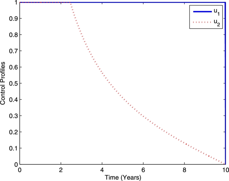
Profile of optimal controls $u_1^{⁎}$ and $u_2^{⁎}$.

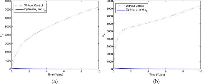
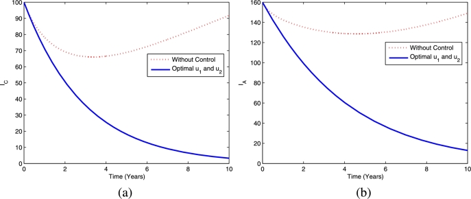
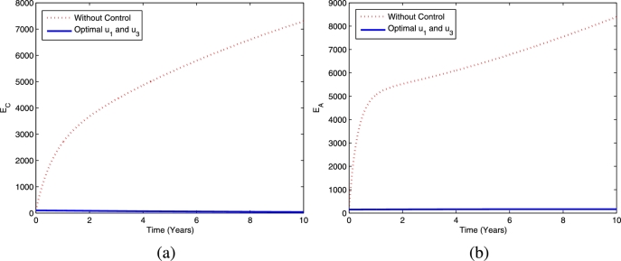
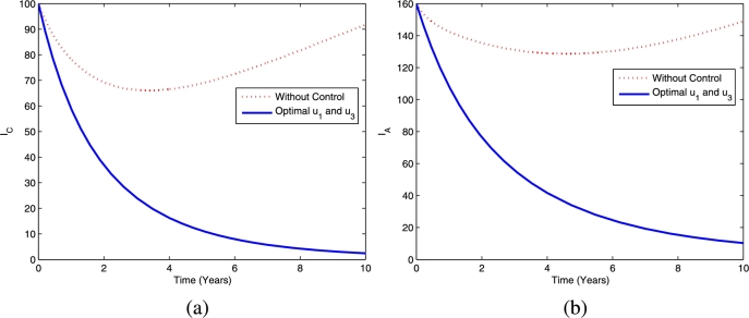
Furthermore, the dynamics of latent TB in the child and adult populations are given in Fig. 4, and the dynamics of active TB in the child and adult populations are given in Fig. 5. Figs. 4(a)-4(b) show that TB prevention and chemoprophylaxis for latent TB controls provide a significant reduction in latent TB in the child and adult populations compared to having no controls. Similar conditions also hold for active TB in the child and adult populations, i.e., active TB in both populations are lower compared to running the model without controls as depicted in Figs. 5(a)-5(b).

Figure 4.

The dynamics of latent TB in children (a) and adults (b) using controls $u_1^{⁎}$ and $u_2^{⁎}$.

Figure 5.

Dynamics of active TB in children (a) and adults (b) using optimal controls $u_1^{⁎}$ and $u_2^{⁎}$.

6.2. Second strategy

In the second strategy, the optimal controls for TB prevention ($u_1^{⁎}$) and TB treatment ($u_3^{⁎}$) are implemented. The profile of the optimal controls $u_1^{⁎}$ and $u_3^{⁎}$ is given in Fig. 6. Using this strategy, TB prevention should be done intensively for nearly 10 years. Meanwhile, TB treatment is at the upper bound of 100% and decreases gradually to lower bound in 10 years.

Figure 6.

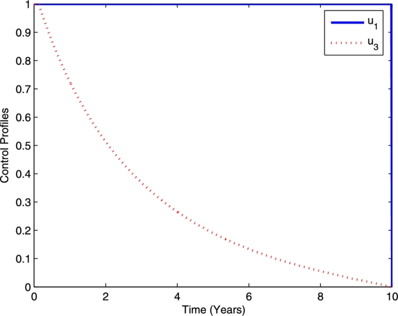
Profile of optimal controls $u_1^{⁎}$ and $u_3^{⁎}$.

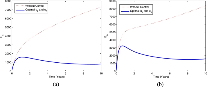
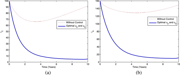
Figs. 7 and 8 provide the dynamics of latent TB infections in the child and adult populations as well as active TB in the child and adult populations, respectively, using the optimal controls $u_1^{⁎}$ and $u_3^{⁎}$. This strategy provides a significant reduction in latent TB in the child and adult populations compared to the scenario without controls. Using this strategy, active TB in the child and adult populations decreases more than it would in the absence of controls.

Figure 7.

The dynamics of latent TB in children (a) and adults (b) using optimal controls $u_1^{⁎}$ and $u_3^{⁎}$.

Figure 8.

The dynamics of active TB in children (a) and adults (b) using optimal controls $u_1^{⁎}$ and $u_3^{⁎}$.

6.3. Third strategy

In the third strategy, we implement the combination of optimal controls for chemoprophylaxis for latent TB ($u_2^{⁎}$) and TB treatment ($u_3^{⁎}$) for simulation. The profile of the optimal controls $u_2^{⁎}$ and $u_3^{⁎}$ is given in Fig. 9. Using this strategy, chemoprophylaxis for latent TB and TB treatment should be done intensively for almost 10 and 9.5 years, respectively, and then decreases to the lower bound.

Figure 9.

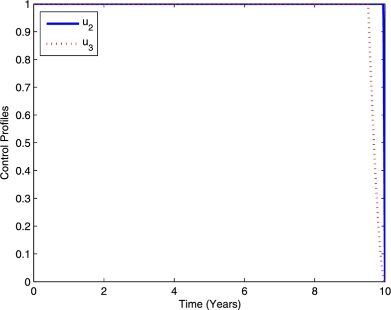
Profile of optimal controls $u_2^{⁎}$ and $u_3^{⁎}$.

Figs. 10 and 11 show the dynamics of latent TB and active TB in the child and adult populations, respectively, using the optimal controls $u_2^{⁎}$ and $u_3^{⁎}$. In utilizing this strategy, we observe in Figs. 10(a)-10(b) that latent TB in both populations is less than the latent TB in both populations when no controls are used. Similarly, in Figs. 11(a)-11(b), we observed that active TB in both populations is lower when the control strategies are adopted than it is without controls.

Figure 10.

The dynamics of latent TB in children (a) and adults (b) using optimal controls $u_2^{⁎}$ and $u_3^{⁎}$.

Figure 11.

The dynamics of active TB in children (a) and adults (b) using optimal controls $u_2^{⁎}$ and $u_3^{⁎}$.

6.4. Fourth strategy

In the last strategy, a combination of optimal controls for TB prevention ($u_1^{⁎}$), chemoprophylaxis for latent TB ($u_2^{⁎}$), and TB treatment ($u_3^{⁎}$) are implemented simultaneously. The profile of the optimal controls is given in Fig. 12. By using this strategy, TB prevention, chemoprophylaxis for latent TB, and TB treatment should be done intensively for almost 10, 2.3, and 1 years, respectively, and then decreased to the lower bound.

Figure 12.

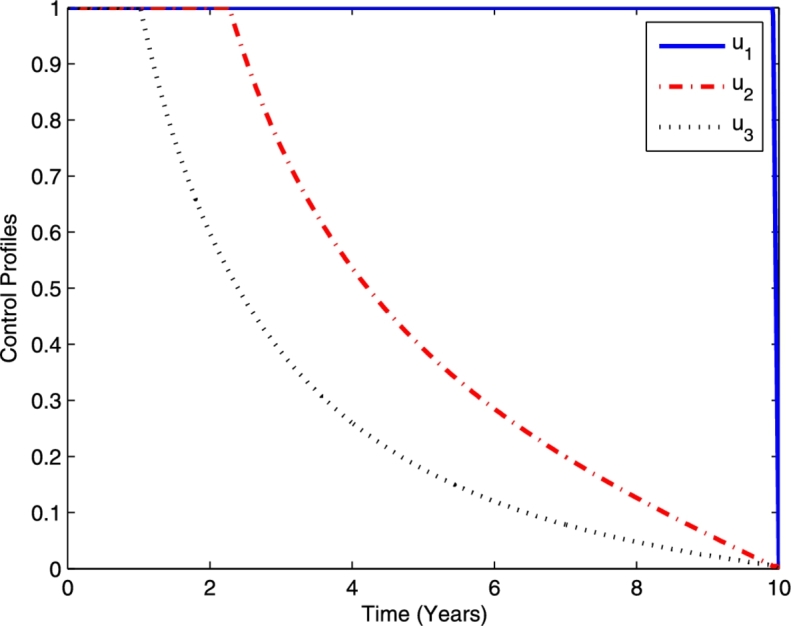
Profile of optimal controls $u_1^{⁎}$, $u_2^{⁎}$ and $u_3^{⁎}$.

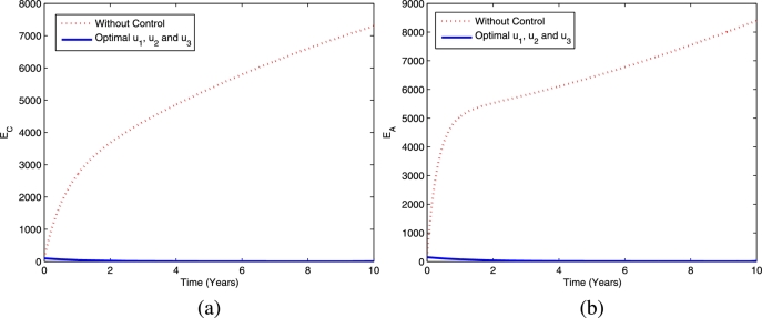
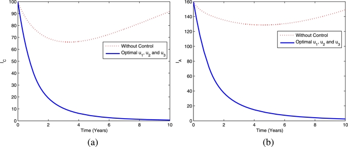
Figs. 13 and 14 provide the dynamics of latent TB and active TB in the child and adult population, respectively, using the fourth strategy. The figures show that this optimal strategy provides a significant reduction in both latent TB and active TB in the child and adult population compared the scenario without controls.

Figure 13.

The dynamics of latent TB in children (a) and adults (b) using optimal controls $u_1^{⁎}$, $u_2^{⁎}$ and $u_3^{⁎}$.

Figure 14.

The dynamics of active TB in children (a) and adults (b) using optimal controls $u_1^{⁎}$, $u_2^{⁎}$ and $u_3^{⁎}$.

Next, we compare the dynamics of models (1) and (2) (the single- and two-age-structured models) for the fourth strategy. First, we expand model (1) by incorporating TB prevention ($u_1$) for the susceptible population (S), chemoprophylaxis ($u_2$) for the latent TB population (E), and TB treatment ($u_3$) for the active TB population (I). The cost function is given by

$$J^s(u_1,u_2,u_3)=\underset{0}{\overset{t_f}{\int }}E+I+\frac{c_1}{2}{u}_1^2+\frac{c_2}{2}{u}_2^2+\frac{c_3}{2}{u}_3^{2}dt.$$ (10)

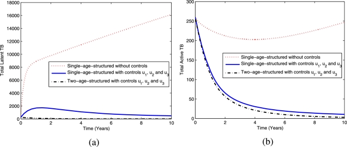
The comparison between the dynamics for latent TB and active TB for the single- and two-age-structured models are shown in Fig. 15. The simulation results of Fig. 15(a) show that the total latent TB population for the two-age-structured model decreases more than the single-age model when using the fourth strategy. Similarly, Fig. 15(b) shows that the total active TB population in the two-age-structured model is less than that for the single-model using this set of controls. The significant reduction indicates that the two-age-structured model is better than the single-age model at controlling the spread of TB in the population.

Figure 15.

The dynamics of total latent TB (a) and active TB (b) using optimal controls $u_1^{⁎}$, $u_2^{⁎}$ and $u_3^{⁎}$.

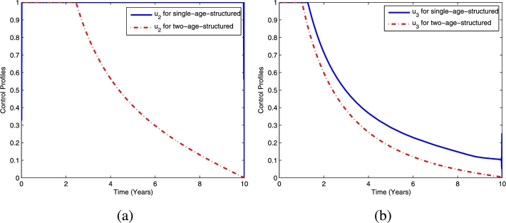
The corresponding control profile for TB prevention ($u_1$) is displayed in Fig. 16, while the chemoprophylaxis ($u_2$) and TB treatment ($u_3$) are presented in Figs. 17(a) and 17(b), respectively. It can be seen from Fig. 16 that the efforts expended on TB prevention for the single- and two-age-structured models are not different. Moreover, from Fig. 17, we can see that the efforts expended on chemoprophylaxis and TB treatment for the single-age-structured model is greater than those expended for the two-age-structured model. The different efforts expended here are due to everyone in one-age-structured model is being treated using the adult rate.

Figure 16.

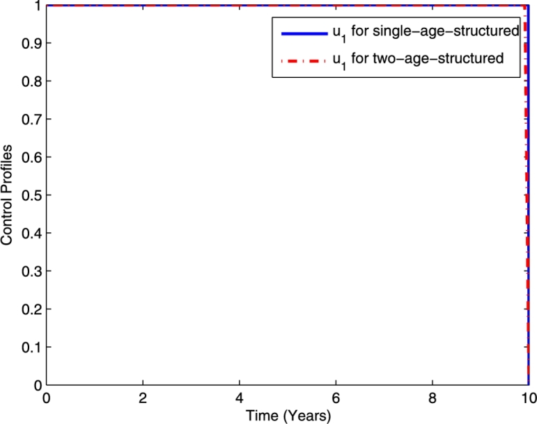
The comparison of the control profiles $u_1^{⁎}$.

Figure 17.

The comparison of the control profiles $u_2^{⁎}$ (a) and $u_3^{⁎}$ (b).

7. Cost-effectiveness analysis

We could not easily determine the best optimal strategy due to the figures in Section 6 exhibiting similar patterns. Meanwhile, the third strategy performed the most poorly (see Figure 10, Figure 11). Here, we conduct a cost-effectiveness analysis to determine the most effective strategy of the four strategies presented in Section 6.

To measure the differences between the costs and health outcomes of these four strategies, we use the incremental cost-effectiveness ratio (ICER) [37], [38], [39]. We use ratio ICER for comparing two intervention strategies that compete for the same resources. Ratio ICER could be interpreted as the additional cost per additional health outcome. When measuring two or more competing strategies incrementally, one intervention should be compared with the next-less-effective alternative [40]. The ICER formula is as follows.

$$\text{ICER}=\frac{\text{Difference in costs produced by strategies}\mathit{\text{i}}\text{and}\mathit{\text{j}}}{\text{Difference in the total number of infection averted in strategies}\mathit{\text{i}}\text{and}\mathit{\text{j}}}.$$

The total number of averted infections is calculated from the difference between the total number of infected individuals without controls and the total infected individuals with controls. Moreover, for the total cost for the implemented strategies, we employed the cost functions, $\frac{c_1}{2}{u}_1^2,\frac{c_2}{2}{u}_2^2$, and $\frac{c_3}{2}{u}_3^2$ over time. We also used the parameter values in Table 3 to compute the total cost and total infections averted, as in Table 5, with an increasing order of total averted infections.

Table 5.

Number of averted infections and total cost of each strategy.

Strategy	Optimal controls	Total averted infection	Total cost
0	no controls	0	0
1	$u_1^{⁎}$, $u_2^{⁎}$	1.2399 ×103	383.3547
2	$u_1^{⁎}$, $u_3^{⁎}$	1.4416 ×103	318.8270
3	$u_2^{⁎}$, $u_3^{⁎}$	1.6452 ×103	782.2304
4	$u_1^{⁎}$, $u_2^{⁎}$, $u_3^{⁎}$	1.7424 ×103	486.8425

The strategy to be excluded at each step is that corresponding to the highest ICER [41]. First, we compared the cost-effectiveness of strategies 1 and 2. The ICERs are calculated as follows.

$$\begin{gathered} \text{ICER(1)}=\frac{383.3547-0}{1.2399\times {10}^3-0}=0.3092 \\ \text{ICER(2)}=\frac{318.8270-383.3547}{1.4416\times {10}^3-1.2300\times {10}^3}=-0.3199. \end{gathered}$$

From the values of ICER(1) and ICER(2), we can observe that strategy 2 is cheaper than strategy 1. In other words, strategy 1 is more costly and less effective than strategy 2. Therefore, strategy 1 is excluded from the set of options, and strategies 2 and 3 are compared.

$$\begin{gathered} \text{ICER(2)}=\frac{318.8270}{1.4416\times {10}^3}=0.2212 \\ \text{ICER(3)}=\frac{782.2304-318.8270}{1.6452\times {10}^3-1.4416\times {10}^3}=2.2760 \end{gathered}$$

Similarly, from the values of ICER(2) and ICER(3), it can be seen that strategy 2 is cheaper than strategy 3. Therefore, strategy 3 should be excluded from the set of options because strategy 3 is more costly and less effective than strategy 2. Hence, we continue on to the comparison of strategies 2 and 4.

$$\begin{gathered} \text{ICER(2)}=\frac{318.8270}{1.4416\times {10}^3}=0.2212 \\ \text{ICER(4)}=\frac{486.8425-318.8270}{1.7424\times {10}^3-1.4416\times {10}^3}=0.5586. \end{gathered}$$

Finally, from the values for ICER(2) and ICER(4), we can observe that strategy 2 is cheaper than strategy 4. Therefore, strategy 4 should be excluded from the set of options since it is more costly and less effective than strategy 2. Hence, we deduce that strategy 2 (the combination of TB prevention and TB treatment only) is the most cost-effective of all the strategies for TB control interventions.

Repeating the iteration process, we can decide the next most cost-effective strategy. Thus, we arrive at strategy 4 being the next most cost-effective strategy after strategy 2, followed by strategy 1, then strategy 3. These findings indicate that strategy 3 is the least effective strategy.

8. Conclusion

In this paper, we constructed epidemic models of TB transmission within single- and two-age-structured populations. From the analysis of the models, we got the basic reproduction ratios that determine the existence and local stability of the equilibria. If the ratios are less than unity, then the disease-free equilibriums are locally asymptotically stable. On the contrary, the disease will endemic in the population whenever the ratios are greater than unity. We also compared the sensitivity indices of the basic reproduction ratios with respect to the parameters of the single- and the two-age-structured models. Finally, we extended the TB transmission model for an age-structured population by applying optimal control strategies.

We simulated the optimal control system by comparing with the system without control. The numerical simulations indicated that control strategies have a significant impact in terms of reducing TB infections in the population. However, the combination of chemoprophylaxis for latent TB and TB treatment has the least impact on TB infection reduction.

From the comparison results for the application of three control variables, it is shown that the total latent and infected populations for the two-age-structured model decreased more than they did in the single-age model. Thus, the effort expended for chemoprophylaxis for latent TB and TB treatment for two-age-structured model is less than that expended for the single model. The greater effort needed in single-age-structured population is due to all patients being managed via adult intervention.

Furthermore, we conducted ICER analysis for cost-effectiveness to deduce the most cost-effective control intervention. From the pairwise comparison results, we conclude that the combination of TB prevention and TB treatment is the most cost-effective strategy to implement. This is followed by the combination of three controls, the combination of TB prevention and chemoprophylaxis for latent TB, then the combination of chemoprophylaxis for latent TB and TB treatment.

Declarations

Author contribution statement

Fatmawati, Hengki Tasman: Conceived and designed the experiments; Performed the experiments; Analyzed and interpreted the data; Wrote the paper.

Utami Dyah Purwati: Analyzed and interpreted the data.

Firman Riyudha: Performed the experiments.

Funding statement

Part of this research is financially supported by the Research Grant Penelitian Berbasis Kompetensi (PBK) 2018.

Competing interest statement

The authors declare no conflict of interest.

Additional information

No additional information is available for this paper.

References

- 1.World Health Organization . World Health Organization; Switzerland: 2016. Global Tuberculosis Report 2016. [Google Scholar]
- 2.World Health Organization Factsheet on the world tuberculosis report, WHO. 2017. http://www.who.int/mediacentre/factsheets/fs104/en/ [Online] Available from.
- 3.Velayati A.A. S1-S2 Sciencedirect: Elsevier; 2016. Tuberculosis in Children. (International Journal of Mycobacteriology). [DOI] [PubMed] [Google Scholar]
- 4.Huo H.F., Zou M.X. Modelling effects of treatment at home on tuberculosis transmission dynamics. Appl. Math. Model. 2016;40:9474–9484. [Google Scholar]
- 5.Liu Q., Jiang D., Shi N., Hayat T., Alsaedi A. Dynamics of a stochastic tuberculosis model with constant recruitment and varying total population size. Physica A. 2017;469:518–530. [Google Scholar]
- 6.Moualeu D.P., Weiser M., Ehrig R., Deflhard P. Optimal control for tuberculosis model with undetected cases in Cameroon. Commun. Nonlinear Sci. Numer. Simul. 2015;20:986–1003. [Google Scholar]
- 7.Ahmadin, Fatmawati Mathematical modeling of drug resistance in tuberculosis transmission and optimal control treatment. Appl. Math. Sci. 2014;8(92):4547–4559. [Google Scholar]
- 8.Silva C.J., Torres D.F.M. Optimal control for a tuberculosis model with reinfection and post-exposure interventions. Math. Biosci. 2013;244(2):154–164. doi: 10.1016/j.mbs.2013.05.005. [DOI] [PubMed] [Google Scholar]
- 9.Silva C.J., Torres D.F.M. Optimal control strategies for tuberculosis treatment: a case study in Angola. Numer. Algebra Control Optim. 2012;2(3):601–617. [Google Scholar]
- 10.Rodrigues P., Silva C.J., Torres D.F.M. Cost-effectiveness analysis of optimal control measures for tuberculosis. Bull. Math. Biol. 2014;76(10):2627–2645. doi: 10.1007/s11538-014-0028-6. [DOI] [PubMed] [Google Scholar]
- 11.Forouzannia F., Gumel A.B. Mathematical analysis of an age-structured model for malaria transmission dynamics. Math. Biosci. 2014;247:80–94. doi: 10.1016/j.mbs.2013.10.011. [DOI] [PubMed] [Google Scholar]
- 12.Aldila D., Götz T., Soewono E. An optimal control problem arising from a dengue disease transmission model. Math. Biosci. 2013;242:9–16. doi: 10.1016/j.mbs.2012.11.014. [DOI] [PubMed] [Google Scholar]
- 13.Mwanga G.G., Haario H., Capasso V. Optimal control problems of epidemic systems with parameter uncertainties: application to a malaria two-age-classes transmission model with asymptomatic carriers. Math. Biosci. 2015;261:1–12. doi: 10.1016/j.mbs.2014.11.005. [DOI] [PubMed] [Google Scholar]
- 14.Tasman H., Supriatna A.K., Nuraini N., Soewono E. A dengue vaccination model for immigrants in a two-age-class population. Int. J. Math. Math. Sci. 2012 15 pages. [Google Scholar]
- 15.Castillo-Chavez C., Feng Z. Global stability of an age-structure model for TB and its applications to optimal vaccination strategies. Math. Biosci. 1998;151:135–154. doi: 10.1016/s0025-5564(98)10016-0. [DOI] [PubMed] [Google Scholar]
- 16.Aparicio J.P., Castillo-Chavez C. Mathematical modelling of tuberculosis epidemics. Math. Biosci. Eng. 2009;6(2):209–237. doi: 10.3934/mbe.2009.6.209. [DOI] [PubMed] [Google Scholar]
- 17.Wang J., Zhang R., Kuniya T. Mathematical analysis for an age-structured hiv infection model with saturation infection rate. Electron. J. Differ. Equ. 2015;30:1–9. [Google Scholar]
- 18.Bonyah E., Dontwi I., Nyabadza F., Fatmawati An age-structured model for the spread of buruli ulcer: analysis and simulation in Ghana. Br. J. Math. Comput. Sci. 2014;4(16):2298–2319. [Google Scholar]
- 19.Cao H., Zhou Y. The discrete age-structured SEIT model with application to tuberculosis transmission in China. Math. Comput. Model. 2012;55:385–395. [Google Scholar]
- 20.Centers for Disease Control and Prevention TB in children in the United States, CDC. 2018. https://www.cdc.gov/tb/topic/populations/tbinchildren/default.htm [Online] Available from.
- 21.Diekmann O., Heesterbeek J.A.P., Metz J.A.J. On the definition and the computation of the basic reproduction ratio in models for infectious diseases in heterogenous populations. J. Math. Biol. 1990;28:362–382. doi: 10.1007/BF00178324. [DOI] [PubMed] [Google Scholar]
- 22.Diekmann O., Heesterbeek J.A.P. John Wiley & Son; 2000. Mathematical Epidemiology of Infectious Diseases, Model Building, Analysis and Interpretation. [Google Scholar]
- 23.van den Driessche P., Watmough J. Reproduction numbers and sub-threshold endemic equilibria for compartmental models of disease transmission. Math. Biosci. 2002;180:29–48. doi: 10.1016/s0025-5564(02)00108-6. [DOI] [PubMed] [Google Scholar]
- 24.Chitnis N., Hyman J.M., Cushing J.M. Determining important parameters in the spread of malaria through the sensitivity analysis of a mathematical model. Bull. Math. Biol. 2018;70:1272–1296. doi: 10.1007/s11538-008-9299-0. [DOI] [PubMed] [Google Scholar]
- 25.Fatmawati, Tasman H. An optimal control strategy to reduce the spread of malaria resistance. Math. Biosci. 2015;262:73–79. doi: 10.1016/j.mbs.2014.12.005. [DOI] [PubMed] [Google Scholar]
- 26.Fatmawati, Tasman H. An optimal treatment control of TB-HIV coinfection. Int. J. Math. Math. Sci. 2016 11 pages. [Google Scholar]
- 27.Okosun K.O., Makinde O.D. A co-infection model of malaria and cholera diseases with optimal control. Math. Biosci. 2014;258:19–32. doi: 10.1016/j.mbs.2014.09.008. [DOI] [PubMed] [Google Scholar]
- 28.Okosun K.O., Makinde O.D. Optimal control analysis of hepatitis C virus with acute and chronic stages in the presence of treatment and infected immigrants. Int. J. Biomath. 2014;7(2) 23 pages. [Google Scholar]
- 29.Pontryagin L.S., Boltyanskii V.G., Gamkrelidze R.V., Mishchenko E.F. Wiley; New York: 1962. The Mathematical Theory of Optimal Processes. [Google Scholar]
- 30.Lewis F.L., Syrmos V.L. John Wiley & Sons; New York: 1995. Optimal Control. [Google Scholar]
- 31.Naidu D.S. CRC PRESS; New York: 2002. Optimal Control Systems. [Google Scholar]
- 32.Lenhart S., Workman J.T. John Chapman and Hall; 2007. Optimal Control Applied to Biological Models. [Google Scholar]
- 33.Bhunu C.P. Mathematical analysis of a three-strain tuberculosis transmission model. Appl. Math. Model. 2011;35:4647–4660. [Google Scholar]
- 34.Agusto F.B. Optimal chemoprophylaxis and treatment control strategies of a tuberculosis transmission model. World J. Model. Simul. 2009;5(3):163–173. [Google Scholar]
- 35.Athithan S., Ghosh M. Optimal control of tuberculosis with case detection and treatment. World J. Model. Simul. 2015;11(2):111–122. [Google Scholar]
- 36.Tewa J.J., Bowong S., Mewoli B. Mathematical analysis of two-patch model for the dynamical transmission of tuberculosis. J. Appl. Math. Model. 2012;36:2466–2485. [Google Scholar]
- 37.Tilahun G.T., Makinde O.D., Malonza D. Modelling and optimal control of pneumonia disease with cost-effective strategies. J. Biol. Dyn. 2017;11(S2):400–426. doi: 10.1080/17513758.2017.1337245. [DOI] [PubMed] [Google Scholar]
- 38.Tilahun G.T., Makinde O.D., Malonza D. Modelling and optimal control of typhoid fever disease with cost-effective strategies. Comput. Math. Methods Med. 2017 doi: 10.1155/2017/2324518. (1–16 pages) [DOI] [PMC free article] [PubMed] [Google Scholar]
- 39.Tilahun G.T., Makinde O.D., Malonza D. Co-dynamics of pneumonia and typhoid fever diseases with cost- effective optimal control analysis. Appl. Math. Comput. 2018;316:438–459. [Google Scholar]
- 40.Okosun K.O., Rachid O., Marcus N. Optimal control strategies and cost-effectiveness analysis of a malaria model. Biosystems. 2013;111:83–101. doi: 10.1016/j.biosystems.2012.09.008. [DOI] [PubMed] [Google Scholar]
- 41.Buonomo B., Marca R.D. Optimal bed net use for a dengue disease model with mosquito seasonal pattern. Math. Methods Appl. Sci. 2017:1–20. [Google Scholar]