Abstract
In this paper, we have developed and analyzed a deterministic Zika model considering both vector and sexual transmission route with the effect of human awareness and vector control in the absence of disease induce death. To formulate the model, we assume that the Zika virus is being first transmitted to human by mosquito bite, and then it is being transmitted to his or her sexual partner. The system contains at most three equilibrium points among them one is the disease free and other two are endemic equilibrium points, exists under certain conditions. The theoretical analysis shows that the diseases-free equilibrium is locally and globally asymptotically stable if the basic reproduction number is less than one. Theatrically we have established that endemic equilibrium point which is locally asymptotically stable if the basic reproduction number is greater than one. The system exhibits backward bifurcation when the transmission probability per biting of susceptible mosquito with infected humans crosses the critical value. We estimate the model parameters and validate the model by fitting the model with the reported Zika infected human data from 1 to 36 week of 2016 Zika outbreak in Colombia. Furthermore, using the normalised forward sensitivity index method we have established that the model parameter mosquito biting rate, recruitment rate of mosquito, transmission probability per biting of Susceptible (infected) humans with infected (susceptible) mosquito, rate of awareness in host population, recovery rates of infected human are most sensitive parameters of the considered Zika model. Lastly, some conclusions are given to control the spreading of the Zika disease.
Keywords: Zika virus, Vector transmission, Sexual transmission, Basic reproduction number, Stability analysis, Backward bifurcation, Sensitivity analysis
1. Introduction
Recently, Zika virus infection has become a dangerous threat for the human society (Cauchemez, 2016; Mlakar, 2016). It is a vector borne disease, spreads through the mosquito borne flavi-virus. In the beginning, the infection transmitted to the human body by the bites of infected Aedes aegypti female mosquitoes, which also transmit the dengue, chikungunya, yellow fever, Japanese Encepalitie’s virus (European Centre for Disease Control and Prevention (CDC), 2015; World Health Organisation(WHO), 2016) widely in the tropical and subtropical regions. Symptoms of Zika infection are normally mild, including fever, headaches, rash, conjunctivitis and joint pain due to flavi-virus. Zika infection increases the chances of microcephaly (permanent disabilities) Guillain-Barre syndrome and other neurological disorder in newborn babies from infected mothers (Cauchemez, 2016; Mlakar, 2016).
This virus was first identified from rhesus monkeys in 1947 in the Zika forest of Uganda (Dick, Kitchen, & Haddow, 1952; Sikka, Chattu, & Popli, 2016) and from humans in Nigeria in 1954 (Dick et al., 1952; Macnamara, 1954; Shapshak, 2015, pp. 477–500) but it was not spread in epidemic form among the human population until 2007 (European Centre for Disease Control and Prevention (CDC), 2015; Duffy, 2009). The first Zika outbreak among human occurred in Yap Island, Micronesia in 2007 (European Centre for Disease Control and Prevention (CDC), 2015; Duffy, 2009; Manore and Hyman, 2016). Afterward, this disease highly spread among human in a different country. First Zika virus, epidemic occurred in French Polynesia in the year 2013–2014 (Hancock, Marfel, & Bel, 2014). After 2015, it is spreading rapidly worldwide. The country Brazil, Southern and Central American as well as in Caribbean, countries are highly affected by Zika. World Health Organisation declared Zika as “public health emergency of the international 2016. According to Pan American Health Organisation (PAHO) and WHO, 583451 suspected and 223477 confirmed cumulative Zika cases were reported up to 04 January 2018 by countries and territories in the Americans among which the respective cases for Brazil are 231725 and 137288 respectively.
Recent studies showed that Zika virus can be transmitted not only by vector only, it also spread by sexual interaction which was reported in (Foy, 2011; Dallas County Health Human Services (DCHHS), 2016; Centres for Disease Control and Prevention (CDC), 2016; The Toronto Star, 2016; Musso, 2015). A remarkable observation was given by the authors in (Musso, 2015) reported that though Zika virus was disappeared from the blood of an infected person even then it was present in his semen, which point out the possibility of sexual transmission of the Zika virus.
Though Zika infection is a threat for public health, but at present no vaccination is available to protect from Zika infection and no particular treatment, medicine or fast diagnostic test is available to treat or diagnose this infection. Thus human awareness through health programs and control of mosquitoes through insecticides is the two effective ways to prevent its infection transmission among the host population.
In the last few years, a number of mathematical models have been reported (Agusto et al., 2017a, 2017b; Bearcroft, 1956; Bonyah, Khan, Okosun, & Islam, 2017; Imran, Usman, Dur-e-Ahmad, & Khan, 2017; Kucharski et al., 2016; Perkins, Siraj, Ruktanonchai, Kraemer, & Tatem, 2016; Shah, Patel, & Yeolekar, 2017) to study the Zika virus transmission dynamics. In those models, the investigators have incorporated the following factors, (i) both vector and sexual transmission (Agusto et al., 2017a, 2017b; Shah et al., 2017), (ii) both vector and sexual transmission route with bilinear incidence rate and they established the backward bifurcation and the global stability of DFE for the same model, but in a single model backward bifurcation and the global stability of DFE are contradictory to each other. (iii) the vertical transmission and vector transmission (Agusto et al., 2017a, 2017b; Imran et al., 2017) and (iv) optimal control on spraying insecticides, other prevention, and treatment (Bonyah et al., 2017; Pontryagin, Boltyanskii, Gamkrelidze, & Mishchenko, 1986; Shah et al., 2017). The impact of awareness on dengue dynamics has been studied by Gakkhar and Chavda (Gakkhar & Chavda, 2013).
In order to study the impact of human awareness and vector control, we construct a Zika model including both vector and sexual transmission route, we also include the human awareness (Mishra & Gakkhar, 2014) and vector control. In this work, we have established the wellposedness, positivity and boundedness, the local and global stability of the DFE and the existence and local stability of endemic equilibrium (EE). Finally, we have validated and estimated the model parameters of the considered model comparing the model predictions with the reported zika infected data of a particular area. To explore the model robustness to parameter values used we investigate the sensitivity analysis using the normalised forward sensitivity index. We also studied numerically the impact of sexual transmission on the epidemic growth rate as well as on the basic reproduction number. To the best of our knowledge effect of vector transmission, sexual transmission, vector control, and human awareness has not yet been considered in a single Zika model. So in this paper, we are considering all these four important facts to propose a Zika model and intend to study its dynamical behaviour.
The rest of the paper is organized as follows: The formulation and basic properties of the model have been described in section-2. An investigation of the stability and bifurcation of the model has been reported in section-3. Parameter estimation and model validation done by simulating the model with reported real data done in section-4. Sensitivity analysis of the model is presented in section-5 and section-6 deals with the effect of sexual transmission on basic reproduction number and epidemic growth rate numerically. Finally, all the results have been concluded in the section-7.
2. Model formulation
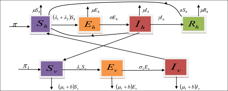
Let the total human population is classified into four compartments comprised of susceptible human , exposed human , infected human and recovered human. Here we have considered that a human individual who recovered from infection of Zika virus gain lifelong immunity from it. Sine only female mosquito spreads the zika infection so the total female mosquito population is divided into three compartments viz. susceptible mosquitoes , exposed mosquitoes and infected mosquitoes . Again recovery of mosquito from Zika infection is not taken into consideration due to its short life span.
To formulate the model the following factors are taken into consideration:
-
(i)
Constant recruitment rate for both susceptible human and vector population.
-
(ii)
Natural death rate for both human and vector population.
-
(iii)
Horizontal transmission of infection from infected vectors to susceptible human when infected vectors bite susceptible human.
-
(iv)
Sexual transmission of infection to susceptible human when a susceptible human interact sexually with an infected human.
-
(v)
Horizontal transmission of infection from infected human to susceptible vectors when susceptible vectors bite infected human.
-
(vi)
Two steps of human awareness has considered. At a constant rate susceptible human can take following awareness steps to protect them from zika (a) using mosquito-nets, and mosquito repellents (b) avoiding sexual interaction or using a condom at the period of zika out break.
-
(vii)
Vector control: spray of insecticide and removal of the stagnant water can control vector.
Let, be the constant recruitment rate of susceptible human and be the natural death rate of the human population. Suppose, susceptible individuals acquire infection due to effective contact with an infected vector at rate , be the infection due to sexual interaction with the infected individuals and susceptible human become aware at a constant rate and enter into recovered class . So the total infection strength of human is .Here we assume that the susceptible mosquitoes acquire infection at a rate from infected human where .
Under the above assumptions, the flow diagram for both human population and vector population of the proposed zika model is given in the following flow diagram (see Fig. 1).
Fig. 1.
Flow diagram of Zika virus in both human and mosquito population.
According to the assumptions and from the flow diagram, the dynamics of the Zika virus can be represented by the following system of non linear differential equations:
| (1) |
The state variables and parameters used in the zika transmission model are summarised in Table 1.
Table 1.
Description of state variables and parameters
| State variables | Description |
|---|---|
| Total human population | |
| Susceptible human population | |
| Exposed human population | |
| Infected human population | |
| Recovered human population | |
| Total vector population | |
| Susceptible vector population | |
| Exposed vector population | |
| Infected vector population | |
| Parameters | Description |
| , | Recruitment rate of human and mosquito respectively |
| , | Natural death rate of human and mosquito respectively |
| Mosquito biting rate | |
| Transmission probability per biting of -Susceptible humans with infected mosquito | |
| Transmission probability per biting of Susceptible mosquito with infected humans. | |
| Sexual contact rate between a susceptible human to an infected human | |
| Transmission probability per sexual contact- among a susceptible and infected human | |
| Progression rate from exposed to infected human | |
| Recovery rate of infected human | |
| Rate of awareness in host population | |
| Progression rate from exposed to infected mosquito | |
| Constant rate of effective mosquito control |
2.1. Positivity and boundedness of the solutions
The considered model will be biologically meaningful when all the variables are non-negative for . In other words the solution with positive initial conditions will remain positive for all time, which we shall establish in the following Lemma.
Lemma 1
Let with the initial condition .Then the solutions of the model (1) is non negative for all . Also andhold.
Proof: Since is a function of and is a function of and for the first equation of the model (1) can be explicitly written as:
Integrating the above equation in the range [0, T] we get,
which gives
or
Similarly it can be shown that and all are positive for all thus for all . Hence the first part of the Lemma is proved.
For the next part of the Lemma it should be noted that
Adding first four component equations of the model (1) we have
| (2) |
Similarly adding last three equations of the model (1) we have
| (3) |
Integrating and taking limsup and liminf for in the above two equations we get, and , which implies and .
We shall now analyze our proposed zika virus transmission model (1) in the following biologically feasible closed region which is defined below:
In the next Lemma we shall establish the closed region as a positively invariant set.
Lemma 2
The closed region defined above is a positively invariant set for the model (1) with non- negative initial condition in.
Proof: Here , so the rate of change of the total human population is
obtained from equation (2) in the form.
Similarly total vector population is , and hence the rate of change of the total mosquito is obtained from (3), as
Using a standard comparison theorem from Lakshmikantham et al. (1989) it can be shown that
and .
This followsand if and respectively.
Thus the closed region is positively invariant.
Again if and then the solution contained in or approach to and approach to and then the infected classes and approach to zero, so is attracting set that is all solutions in eventually enters in . So, biologically and mathematically the model is well posed in the invariant set (Hethcote, 2000). Hence, it is sufficient to consider the dynamics of the transmission of zika virus model (1) in the invariant set .
3. Steady state analysis
In this section we shall carry out qualitative analysis of the model (1) to investigate existence and stability of the steady states.
3.1. Disease free equilibrium and basic reproduction numbers
The disease free equilibrium (DFE) of the model (1) is obtained by using in the steady state conditions.
Thus the disease free equilibrium point of the model (1) is given by .
In order to calculate the basic reproduction number we use the next generation operator method on the model (1). Consider the infected compartments at the disease free equilibrium (DFE) and applying Vanden Diressche and Watmaugh (Van den Driessche & Watmough, 2002) technique, the Jacobian matrices and (for the new infection terms and the remaining transfer terms respectively) are given by.
, so that Now, the basic reproduction number is obtained as the spectral radius (Van den Driessche & Watmough, 2002) that is the dominant Eigen value of the matrix .
The characteristic polynomial of the matrix is where and the quadratic polynomial of the above characteristic polynomial is with .So gives a unique positive root, which provides the basic reproduction number given below:
.
Again and. Define that is where is the contribution from sexual transmission and is the contribution from mosquito (vector) transmission. Again from the relation we have the following three observation:
-
(i)
when then thus the positive root of the equation is one i.e (ii) when then so the positive root of the equation lies between zero and one as thus .(iii) when then again so positive root of greater than one that is . Thus from the above three observation one can conclude that if and only if . Since two threshold numbers and are equivalent so we use only in the next part of the paper.
3.2.1. Local stability of the disease free equilibrium
Lemma 3
The disease free equilibrium (DFE) is locally asymptotically stable for and unstable for where is defined in the text.
Proof. The variational matrix of the model (1) at the disease free equilibrium is given by
The characteristic roots corresponding to matrix are and the remaining four roots are roots of the following equation:
(4) Now by the Routh-Hurtwiz criteria the eigen values of the block matrix will be negative or have negative real part if and . All these conditions will be satisfied if . Thus by Routh-Hurtwiz criteria the disease free equilibrium (DFE) is locally asymptotically stable if . Thus the disease free equilibrium (DFE) is locally asymptotically stable for otherwise it is unstable.
Using the Lemma-3 we can say that zika virus can be eliminated from the population when can be brought to a value less than unity. It is clear from the expression of that with the increase of both the rate of awareness () in host population and the rate of effective mosquito control () decreases. Thus the factors and help us to keep the value of below unity and increase the range of stability of the disease free equilibrium. Thus we can speak that awareness in host population and vector control helps the society to eliminate zika virus from human population.
3.2.2. Global asymptotic stability of the disease free equilibrium
In this section we have studied the global asymptotic stability of the disease free equilibrium (DFE) to ensure that the elimination of zika virus i.e. elimination of disease is independent of the initial sizes of the subpopulations of the model. For this purpose we consider the feasible region where and to establish the invariance of the region we shall establish the following Lemma.
Lemma 4
The region is a positively invariant for the model (1).
Proof: From the first equation of the model (1) we have
as which gives . Thus if for all then for all
Again from the fifth equation of the model (1) we have
Which gives . Thus if for all then for all .
Summing above two we have the region is positively invariant and attracts all solutions in for the model (1). In the next theorem we have studied the global asymptotic stability of .
Theorem 1
The disease free equilibrium of the model (1) is globally asymptotically stable (GAS) in whenever .
Proof: Let and and grouping the model (1) into
where is obtained from the right hand side of first, fourth and fifth equations of the model (1) with and is obtained from the right hand side of second, third, sixth and seventh equations of the model (1).
Now considering the reduced model:
(5) Let be the equilibrium of the reduced model (5). Now we shall show that is a globally stable equilibrium in .To prove this we solve the equations (5) which gives:
and
Thus as .
This asymptotic nature is independent of initial conditions in . Hence the convergence of solutions of (2) is global in . Next we require is to satisfy the following two conditions given in Castill-Chavez et al (Castillo-Chavez, Blower, Van den Driessche, Kirschner, & Yakubu, 2002), namely
1. and 2 . Where and is the Jacobian of with respect to is calculated at .
It is an M-matrix that is off diagonal elements of the matrix are non-negative. The relation gives
In the region and hence we get . Thus, if the human population is at equilibrium level then we have therefore . So by the theorem in Castilo-Chavez et al (Castillo-Chavez et al., 2002) the disease free equilibrium is globally asymptotically stable as the human population is constant in the absence of disease induced death. The biological significance of the above theorem is that the zika virus can be eliminated from the population if can be brought down to a value less than or equal to unity what so ever the size of the initial subpopulation in each class.
3.3. Existence and stability of endemic equilibrium point
In this part we shall find conditions for the existence and stability of endemic equilibrium for the model (1). Let be an arbitrary endemic equilibrium of the model (1) which have been obtained from the steady states of the model, where the components of are given below:
with
| (6) |
| (7) |
The expressions of represent the forces of infection of mosquitoes and human at steady state. Substituting the value of from (6) in (7) and simplifying we get the quadratic equation satisfied by in the form:
| (8) |
where The endemic equilibrium of the model (1) can be obtained by solving the quadratic equation (8) for and substituting into (l). From the expression of it is clear that is always positive and is positive if . Since equation (8) is a second degree equation in , depending on values of the number of endemic equilibrium point will be generated. Thus from the above discussions we can summarize the following theorem:
Theorem 2
The model (1) has
- (a)
An endemic equilibrium if or that is .
- (b)
A unique coincident endemic equilibrium if c1<0 and .
- (c)
Two endemic equilibria exists if that is , and
- (d)
No endemic equilibrium exist other case.
Theorem 3
If then the endemic equilibrium of the model (1) is locally asymptotically stable.
Proof: To prove this theorem we shall use the Krasnoselskii sub linearity trick method (Esteva & Vargas, 2000; Hethcote & Thieme, 1985). Here we shall prove that the linearized part of (1) around the endemic equilibrium has no solution of the form
(9) with and where is the set of complex numbers.
From the system of equations (1) we consider the following subsystem:
(10) Linearizing (10) around the endemic equilibrium we get
(11) The jacobian of the linear system (11) at is
where .
Substitution of a solution of the form (9) in the linearized model (11) yields the following linear equations:
(12) Solving for from second, third and fifth equation of (12) and then substituting these results into its first and fourth equations we get the following equivalent system:
(13) Adding the first and third equations of (13) and removing the negative term of the left hand side (Esteva, Gumel, & de Leon, 2009) we get the following system of equations:
(14) where, and , where
Here the notationrepresent the i-th co-ordinate of the vector. It should be noted that the matrix has non-negative entries and the endemic equilibrium satisfies . If is a solution of (14) then it is possible to find a minimal positive number such that
(15) where . Here the numberis also the minimal positive number that satisfies the inequality . We want to show that . On the contrary we assume and we consider the two cases: and .
In first case the system of equations (12) is homogeneous linear system of equations. It is clear that the coefficient determinant is non zero and consequently the system (12) has the unique solution which corresponds to the disease free steady state of the system (1).
Next we consider the second case . By the assumption , we have which implies that for all. Let us now define .Then or equivalently . The property of minimality of implying . Now taking norms of both sides of the second equation of (14) we get
(16) This inequality implies which contradicts. Hence . Thus the real parts of all eigenvalues of the characteristic equation of the linear system (1) will be negative. So is locally asymptotically stable.
3.4. Backward bifurcation
In this section we shall study the possibility of a backward bifurcation in the zika model (1) using centre manifold theorem as discussed by in Castillo-Chavez and Song (Castillo-Chavez & Song, 2004).
Theorem 4
The model (1) undergoes backward bifurcation at whenever the sign of the coefficient is positive where is defined in (18).
Proof: We redefine the model (1) by changing the variables:
Let . So that
Applying vector notation the model (1) can be written as
where as follows:
(17) For the above system the disease free equilibrium (DFE) given by where
The jacobian matrix of the above system at the disease free equilibrium is given by
Taking as a bifurcation parameter we found , which gives. The jacobian of the transformed model (17) at the disease free equilibrium at has a simple zero eigenvalue and all other eigenvalues have negative real part. So the centre manifold theory can be used to study the dynamics of the model (17) near .In particular we will use the theorem given by Castillo-Chavez and Song (Castillo-Chavez & Song, 2004). The necessary computation for the theorem given bellow:
The right eigenvector:
The right eigenvector of the jacobian associated with zero eigenvalue at is given by: where,
The left eigenvector of the jacobian matrix associated with zero eigenvalue at is given by
where , . The bifurcation coefficients andare given by where and all others derivatives are zero so that
(18) the value of as and the only non-zero derivative is . Therefore .
Hence the model (1) undergoes backward bifurcation at whenever .
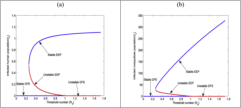
In backward bifurcation a stable disease free equilibrium (DFE) co-exists with two endemic equilibrium (EE) among which one is unstable and other one is stable when .The biological significance of the backward bifurcation phenomenon of the zika model (1) is that the condition for elimination of zika from population is the necessary condition but not sufficient, in that case elimination of zika depend on initial sizes of the population that fact is present in Fig. 2.
Fig. 2.
Backward bifurcation diagram of the modified zika model (17) for: (a) infected human (b) infected mosquito population using the parameter valuesand the values of the other parameters presented inTable 3.
4. Model fitting to the Zika infected data in Colombia: Parameter Estimation and Model validation
In this section we have validated the considered Zika model (1) considering the reported Zika infected human data of 1 to 36 weeks 2016 in Colombia which is given in Table 2. The data has been provided by National Institute of Health SIVIGILA, Colombia which also has been used in literature (Aranda, Gonzalez-Para, & Benincasa, 2019). We found the best fitted model parameters for the considered model (1) with the above said data by using MATLAB minimization software package fmincon. In order to fit the model (1) to the weekly reported Zika infected data in Colombia to the year 2016 we considered the initial susceptible human as 19471223 and the initial number of infected populations as 2173 as reported in (Aranda et al., 2019) and initial density of the other populations we assume arbitrarily. Similarly, some model parameters are assumed arbitrarily and then using the MATLAB minimization software package the remaining parameters have been estimated and those values summarized in Table 3.
Table 2.
The weekly reported data of Zika infection cases in Colombia from 1 to 36 week of 2016 provided by National Institute of Health SIVIGILA, which also used in (Aranda et al., 2019).
| Week | Cases | Week | Cases | Week | Cases | Week | Cases |
|---|---|---|---|---|---|---|---|
| 1 | 2173 | 10 | 2655 | 19 | 3281 | 28 | 705 |
| 2 | 4105 | 11 | 2639 | 20 | 638 | 29 | 648 |
| 3 | 4166 | 12 | 3882 | 21 | 1567 | 30 | 496 |
| 4 | 4669 | 13 | 3808 | 22 | 2014 | 31 | 416 |
| 5 | 4198 | 14 | 3059 | 23 | 1539 | 32 | 215 |
| 6 | 4316 | 15 | 3364 | 24 | 1344 | 33 | 301 |
| 7 | 5460 | 16 | 2671 | 25 | 1128 | 34 | 271 |
| 8 | 2865 | 17 | 2665 | 26 | 991 | 35 | 568 |
| 9 | 3767 | 18 | 2687 | 27 | 892 | 36 | 383 |
Table 3.
Parameter values and their Sensitivity indices of the model (1) with respect to.
| Parameter | Values | Source | Sensitivity index |
|---|---|---|---|
| 0.45 | Agusto et al. (2017a, 2017b) | 1.99928242 | |
| 0.00019204 | Estimated | 1.01880565 | |
| 100 | Assume | 0.99964121 | |
| 0.04441746 | Estimated | 0.99964121 | |
| 0.04791129 | Estimated | 0.99964121 | |
| 0.02070591 | Estimated | 0.50624931 | |
| 0.35808521 | Estimated | ||
| 0.03362689 | Estimated | ||
| 0.00552894 | Estimated | ||
| 0.01747 | Kucharski et al. (2016) | −0.99964121 | |
| 0.07098011 | Estimated | −0.99730175 | |
| 0.00000440 | Estimated | −0.02239870 | |
| 0.02053120 | Estimated | – | |
| 0.00071429 | Assume | – |
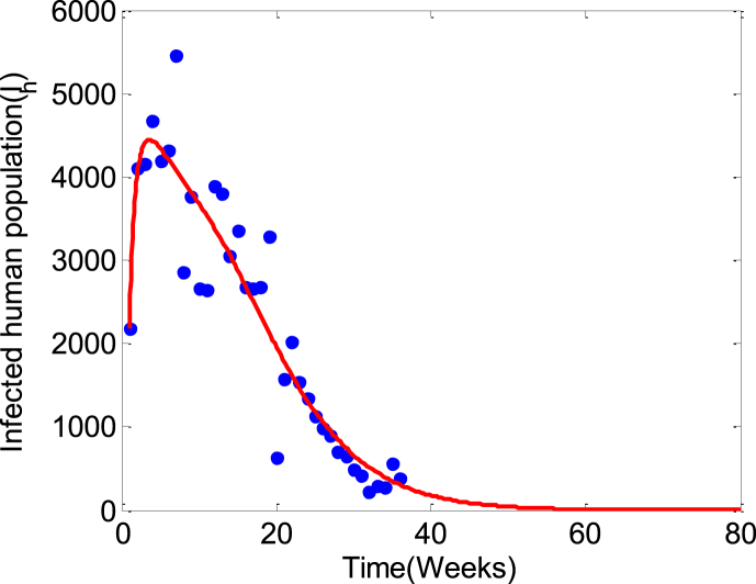
In Fig. 3 we have plotted the reported Zika infection data in Colombia from 1 to 36 week of 2016 using blue dots and considering the estimated model parameters we have predicted the density of the infected populations up to 80 weeks. It is clear from the prediction of the solution curve that the disease will no longer out break after 50 weeks in Colombia, which is supported by the reported real cases in the same region by WHO (Zika-Epidemiological Repo, 2017) . Our model we predict that there will be 113 average weekly cases during 37 to 52 week of the year 2016 which is close to 130 reported real cases by WHO (Zika-Epidemiological Repo, 2017). According to our model prediction zika will be eradicated from Colombia on or after 28 week of 2017 which also supported by real data (Zika-Epidemiological Repo, 2017).
Fig. 3.
The reported infected populations (the blue dots) and the best. fitted solution (solid red curve) the model (1).
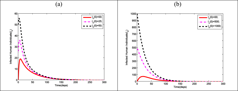
The theoretical finding in Lemma-3, 4 and theorem-1are graphically verified considering the model parameters as given Table 3 (see Fig. 4). For these values of the parameters the value of basic reproduction number is less than unity. Hence the disease free equilibrium point is globally asymptotically stable for these parametric values. In Fig. 4 we have presented the time series of and for different initial values of the populations. It is clear that if the system starts for different initial points then it will ultimately converge to and respectively. Thus from the Fig. 4 it clear that system is locally as well globally asymptotically stable if the condition stated in the corresponding lemmas and theorem is satisfied.
Fig. 4.
Time series for (a) infected humanand (b) infected mosquitopopulations for the parameters given inTable 3with different initial conditions for the model (1).
Since the system contains fourteen parameters among them some parameters are highly sensitive. A small change of the parameters will affect highly the system. In this next section using sensitivity analysis we shall determine the highly sensitive parameters.
5. Sensitivity analysis
Using sensitivity analysis we shall determine the parameters those have high significant impact on the threshold number of the zika model (1). Such analysis tells us the importance of each parameter on disease transmission and this will help the public helth authorities to place of priority for prevention and controlling the spread of the zika virus in the human population. Such information is also important for experimental design, data assimilation and reduction of complex nonlinear model (Powell, Fair, Le Claire, Moore, & Thompson, 2005).
In order to perform such analysis we shall use the normalised forward sensitivity index of a variable with respect to a parameter which is expressed as the ratio of the relative variation in the variable to the relative variation in the parameter. The sensitivity index can be defined using partial derivatives.
Definition 4.1
The normalised forward sensitivity index of that depends differentiably on a parameter is defined by (Chitnis, Hyman, & Cushing, 2008).
Using the explicit expression of in the above sensitivity index formula we have derived an expression for the sensitivity of with respect to each parameter. Then using the base line values of parameters, given in Table 3 we have estimated the numerical values for the sensitivity index and the results are also summarised in Table 3.
A small variation in a most sensitive parameter will create large quantitative variation. Thus it should be carefully estimated whether a small variation in a least sensitive parameter will not create large variation so it need not require too much effort to estimate such least sensitive parameters.
Table 3 presents the base line value of parameters used for the numerical simulation and it also shows the sensitivity indices of the zika model with respect to. From Table 3 it is clear that the mosquito biting rate is the most sensitive parameter with sensitivity index 1.999 which indicates that increase (or decrease) the mosquito biting rate by 10% will be followed by an immediate increase (or decrease) in by 19.99%. Similarly increase (or decrease) of the parameters by 10% will be followed by an immediate increase (or decrease) in by 9.99%, 9.99%, 9.99%, 5.56% respectively.
Though the recruitment rate of human has the most negative sensitivity index but in the epidemiological context the important parameters which have negative sensitivity indices are . The significance of negative sensitivity indices of the above said parameters are increase (or decrease) in the parameters by 10% will be followed by an immediate decrease (or increase) in by 9.97%, 0.224% respectively. In summary, the zika sensitivity analysis identifies the most important parameters driving the transmission mechanism of the zika virus. The results suggest that a control strategy that reduces the mosquito biting rate, recruitment rate of mosquito, transmission probability per biting of susceptible humans by infected mosquito, transmission probability per biting of susceptible mosquito with infected humans, progression rate from exposed to infected mosquito, progression rate from exposed to infected human, transmission probability per sexual contact among a susceptible and infected human and sexual contact rate between a susceptible human to an infected human () respectively and the control strategy that increase rate of recovery rate of infected human, awareness in host population, death rate of mosquito and constant rate of effective mosquito control () will effectively resist the spread of zika virus in the human population.
Now, to verify the sensitive parameters we have plotted the solution curve for the number of infected and exposed humans for different values of the model parameters keeping the initial conditions same. To simulate the system numerically we have to use the estimated model parameter as presented in Table 3 with the initial conditions: .
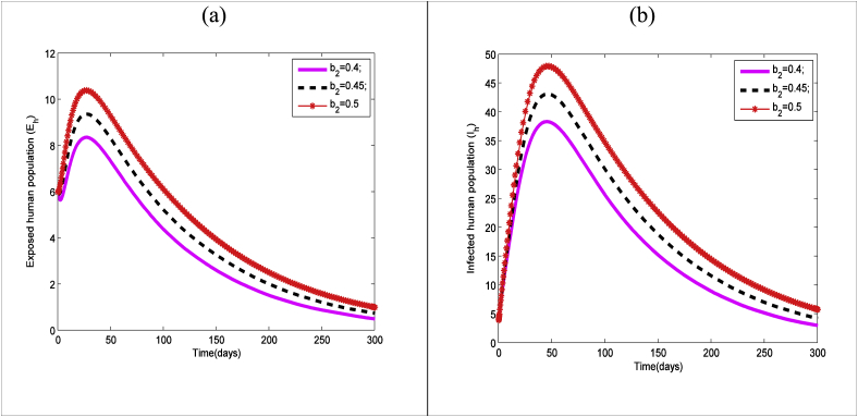
The time series of exposed human and the infectious human are plotted in Fig. 5(a) and (b) respectively for different values of mosquito biting rate (). It is clear from the figures that the number of both class increases due to the increase (decrease) in . Thus the mosquito bite rate plays an important role to spreads the zika virus.
Fig. 5.
Time series of the model (1) for the different values of of (a) Exposed human population (b) infected human population, other parameter values presented in Table 3.
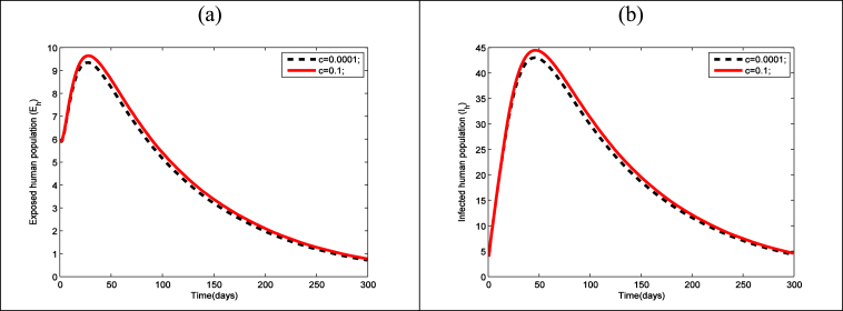
The effect of sexual contact rate () between a susceptible human and an infected human on exposed and infectious human population has been presented in Fig. 6(a) and (b) respectively. It is clear from Fig. 6(a and b) that due to increase or decrease of sexual contact rate () both the exposed and infectious human population increases or decreases.
Fig. 6.
Time series presenting the effect of Sexual contact rate between a susceptible human to an infected human on the (a) exposed human and (b) infected human, using the parameter values presented in Table 3.
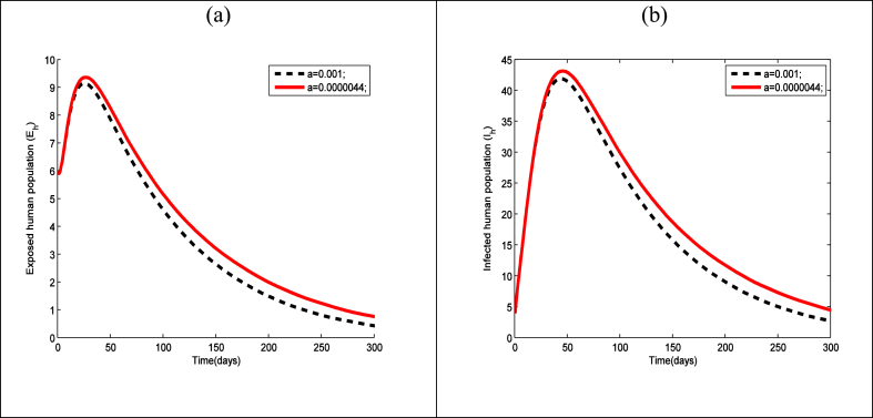
The effect of human awareness rate () on zika transmission dynamics among human presented in Fig. 7(a and b). From these two figures it is clear that increase of human awareness decreases both exposed and infectious human population and vice-versa.
Fig. 7.
Time series of Zika model (1) for different values of human awareness and other parameter values presented in Table 3: (a) exposed human and (b) infected human.
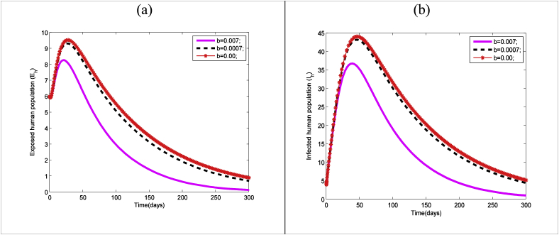
In Fig. 8 we have presented the time series of exposed human and infected human for different values of vector control (). It is clear from the figure that both the exposed human population and infectious human population decrease as the vector control increase.
Fig. 8.
Time series of the Zika model (1) showing the effect of vector control on the (a) exposed human and (b) infected human using the parameter values presented in Table 3.
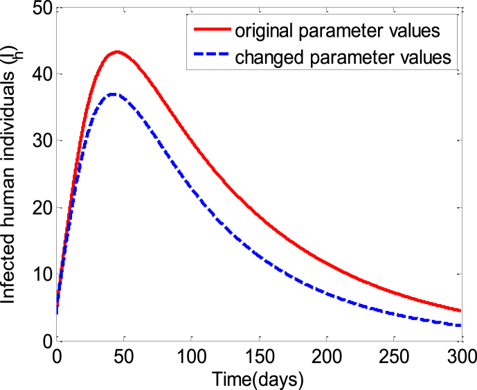
Thus from the above series of time series analysis it is clear that the amount of exposed and infected human population decrease when the vector biting rate (), the sexual contact rate () among susceptible human to infected human decrease and the human awareness rate the vector control rate () increase. Considering above said four facts simultaneously as a precautionary measures we presents the behaviour of the infected human population in Fig. 9. The figure shows that the number of infected human population decreases when the vector biting rate and the sexual contact rate decreases and the human awareness rate and the vector control rate increases simultaneously over a period of time.
Fig. 9.
Time series of the zika model (1) presenting the effect of vector biting rate, sexual contact rate, human awareness and vector control simultaneously on the behaviour of the infected human population. The solid line graphics obtained using the parameter values and the dashed line graphics obtained by using the parameter values the other parameter values presented in Table 3.
6. Effect of sexual transmission on epidemic growth rate and basic reproduction number
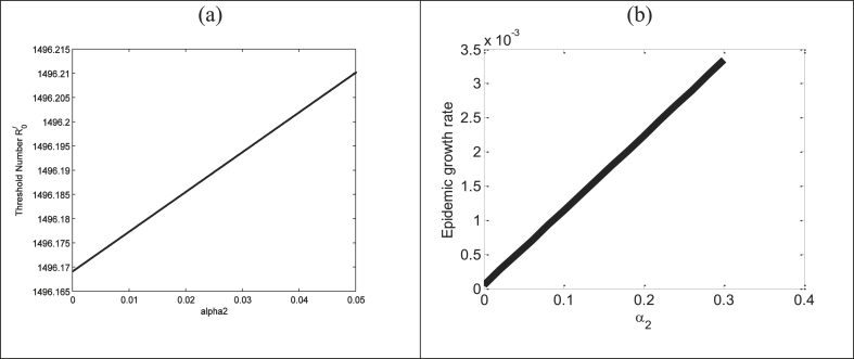
In this section we have established the effect of sexual transmission to the epidemic growth rate as well as basic reproduction number. In deterministic epidemic model the disease free equilibrium (DFE) locally stable if the basic reproduction number and unstable if (Van den Driessche & Watmough, 2002) and for disease outbreak occurs. The dominant eigen value of the jacobian matrix at the disease free equilibrium (DFE) is the initial outbreak growth rate (). In our model the dominant eigenvalue of the jacobian matrix at the DFE is the dominant root of the corresponding characteristic equation (4). It is a four degree equation, so it is not easy to find the explicit expression of the dominant root i.e.to find the initial epidemic growth rate of the model. So, we shall establish the effect of sexual transmission on epidemic growth rate and basic reproduction number numerically. In Fig. 10(a) and (b) we have presented the effect of on the basic reproduction number and the epidemic growth rate respectively. Fig. 10(a and b) show that the basic reproduction number and the epidemic growth rate both increase with the increase of the transmission probability per sexual contact between susceptible and infected human.
Fig. 10.
Presents the effect of on (a) the basic reproduction number and on (b) the epidemic growth rate using the parameter values and the values of the others parameter presented in Table. 3.
7. Conclusion
In this work, we have developed and analyzed a deterministic ODE model for Zika virus transmission dynamics that incorporates both mosquito and sexual transmission paths, which also includes vector control and human awareness. The positivity and boundedness of the proposed model are investigated here. We obtained the basic reproduction number by next-generation matrix technique. The steady-state analysis shows that the disease-free equilibrium (DFE) is and globally asymptotically stable if the basic reproduction number less than unity. The conditions for the existence of endemic equilibrium of the model are obtained. Using the Krasnoselskii sub linearity trick method we have established that the endemic equilibrium is locally asymptotically stable if the basic reproduction number is greater than one. Under some condition the model exhibits the phenomenon of backward bifurcation. The biological significance of this result is that the condition reproduction number less than unity for the elimination of zika virus from the population is the necessary condition but not sufficient. We estimate the model parameters and validate the model by using the reported Zika infection data in Colombia of the year 2016.
The effect of sexual transmission both on basic reproduction number and epidemic growth rate have been established numerically which shows that with the increase of sexual transmission rate the density of exposed and infected populations both increases. So we can control zika virus by controlling sexual transmission rate. Sensitivity and numerical analyses were done to determine the impact of the parameters on the zika infection. The most effective parameters were found the mosquito biting rate, recruitment rate of mosquito, transmission probability per biting of a susceptible human with an infected mosquito, the rate of the awareness host population and the recovery rate of the infected human population. This model will help the public health planar to frame a policy for controlling Zika. In further, we will extend the model incorporating the optimal control theory.
Declaration of competing interest
The Authors have no conflict of interest regarding the model and methodology.
Handling editor: Yiming Shao
Footnotes
Peer review under responsibility of KeAi Communications Co., Ltd.
Contributor Information
Sudhanshu Kumar Biswas, Email: sudhanshukumarbiswas207@gmail.com.
Uttam Ghosh, Email: uttam_math@yahoo.co.in.
Susmita Sarkar, Email: susmita62@yahoo.co.in.
References
- Agusto F.B., Bewick S., Fagan W.F. Mathematical model for Zika virus dynamics with Sexual transmission route. Ecological Complexity. 2017;29:61–81. [Google Scholar]
- Agusto F.B., Bewick S., Fagan W.F. Mathematical model of Zika virus with vertical transmission. Infectious Disease Modelling. 2017;2:244–267. doi: 10.1016/j.idm.2017.05.003. [DOI] [PMC free article] [PubMed] [Google Scholar]
- Aranda L.D.F., Gonzalez-Para G., Benincasa T. Mathematical modelling and numerical simulations of Zika in Colombia considering mutation. Mathematics and Computers in Simulation. 2019;163:1–18. [Google Scholar]
- Bearcroft W.G.C. Zika virus infection experimentally induced in human volunteer. Transactions of the Royal Society of Tropical Medicine & Hygiene. 1956;50(5):442–448. [PubMed] [Google Scholar]
- Bonyah E., Khan M.A., Okosun K.O., Islam S.A. Theoretical Model for Zika virus transmission. PLoS One. 2017;12(10) doi: 10.1371/journal.pone.0185540. [DOI] [PMC free article] [PubMed] [Google Scholar]
- Castillo-Chavez C., Blower S., Van den Driessche P., Kirschner D., Yakubu A.A. Springer-Verlag New York; 2002. Mathematical approaches for emerging and reemerging infectious diseases. [Google Scholar]
- Castillo-Chavez C., Song B. Dynamical model of tuberculosis and their applications. Mathematical Biosciences and Engineering. 2004;1(2):361–404. doi: 10.3934/mbe.2004.1.361. [DOI] [PubMed] [Google Scholar]
- Cauchemez S. Association between Zika virus and microcephaly in Frence Polynesia,2013-2015:a retrospective study. Lancet Published online march. 2016;15 doi: 10.1016/S0140-6736(16)00651-6. [DOI] [PMC free article] [PubMed] [Google Scholar]
- Centres for Disease Control and Prevention (CDC) 23 February 2016. Update : Interim guidelines for prevention of sexual transmission of zika virus-United States, 2016. [Google Scholar]
- Chitnis N., Hyman J.M., Cushing J.M. Determining important parameters in the spread of malaria through the sensitivity analysis of a mathematical model. Bulletin of Mathematical Biology. 2008;70(5):1272–1296. doi: 10.1007/s11538-008-9299-0. [DOI] [PubMed] [Google Scholar]
- Dallas County Health Human Services (DCHHS) 2 February 2016. DCHHS reports first zika virus case in Dallas county acquired through sexual transmission. [Google Scholar]
- Dick G.W., Kitchen S.F., Haddow A.J. Zika virus (I). Isolations and serological specificity. Transmission of the Royal Society of Tropical Medicine and Hygiene. 1952;46:509–520. doi: 10.1016/0035-9203(52)90042-4. [DOI] [PubMed] [Google Scholar]
- Duffy M.R. Zika virus outbreak on Yap Island, Federated States OF Micronesia. New England Journal of Medicine. 2009;360:2536–2543. doi: 10.1056/NEJMoa0805715. [DOI] [PubMed] [Google Scholar]
- Esteva L., Gumel A.B., de Leon C.V. Qualitative study of transmission dynamics of drug-resistant malaria. Mathematical and Computer Modeling. 2009;50:611–630. [Google Scholar]
- Esteva L., Vargas C. Influence of vertical and mechanical transmission on the dynamics of dengue disease. Mathematical Biosciences. 2000;167:51–64. doi: 10.1016/s0025-5564(00)00024-9. [DOI] [PubMed] [Google Scholar]
- European Centre for Disease Control and Prevention (CDC) Factsheet for Health Professionals; 2015. Zika virus infection. [Google Scholar]
- Foy B.D. Probable non-vector-borne transmission of zika virus, Colorado, USA. Emerging Infectious Diseases. 2011;17:880–882. doi: 10.3201/eid1705.101939. [DOI] [PMC free article] [PubMed] [Google Scholar]
- Gakkhar S., Chavda N.C. Impact of awareness on the spread of Dengue infection in human population. Applied Mathematics. 2013;4:142–147. [Google Scholar]
- Hancock W.T., Marfel M., Bel M. Zika virus ,French Polynesia, south pacific, 2013. Emerging Infectious Diseases. 2014;20:1085–1086. doi: 10.3201/eid2011.141253. [DOI] [PMC free article] [PubMed] [Google Scholar]
- Hethcote H.W. The mathematics of infectious diseases. SIAM Review. 2000;42(4):599–653. [Google Scholar]
- Hethcote H.W., Thieme H.R. Stability of the endemic equilibrium in epidemic models with subpopulations. Mathematical Biosciences. 1985;75:205–227. [Google Scholar]
- Imran M., Usman M., Dur-e-Ahmad M., Khan A. Transmission dynamics of zika fever: A SEIR based model. Differential Equations and Dynamical Systems. 2017 [Google Scholar]
- Kucharski A.J., Funk S., Eggo R.M., Mallet H., Edmunds W.J., Nilles E.J. Transmission dynamics of zika virus in Island population : A modelling analysis of the 2013-2014 French Polynesia outbreak. PLoS Neglected Tropical Diseases. 2016;10(5) doi: 10.1371/journal.pntd.0004726. [DOI] [PMC free article] [PubMed] [Google Scholar]
- Lakshmikantham V., Leela S., Martynyuk A.A. Marcel Dekker. Inc.; New York and Basel: 1989. Stability analysis of nonlinear system. [Google Scholar]
- Macnamara F.N. Zika virus: A report on three cases of human infection during an epidemic of jaundice in Nigeria. Transactions of the Royal Society of Tropical Medicine & Hygiene. 1954;48(2):139–145. doi: 10.1016/0035-9203(54)90006-1. [DOI] [PubMed] [Google Scholar]
- Manore C, and Hyman M, Mathematical models for fighting Zika virus, SIAM news, Retrieved May 2, 2016.
- Mishra A., Gakkhar S. The effects of awareness and vector control on two strains dengue dynamics. Applied Mathematics and Computation. 2014;246:159–167. [Google Scholar]
- Mlakar J. Zika virus associated with microcephaly. New England Journal of Medicine. 2016;374(10):951–958. doi: 10.1056/NEJMoa1600651. [DOI] [PubMed] [Google Scholar]
- Musso D. Potential sexual transmission of Zika virus. Emerging Infectious Diseases. 2015;21(2):359–361. doi: 10.3201/eid2102.141363. [DOI] [PMC free article] [PubMed] [Google Scholar]
- Perkins T.A., Siraj A.S., Ruktanonchai C.W., Kraemer M.U.G., Tatem A.J. 2016. Model-based projection of Zika virus infections in childbearing women in the Americas, biorxiv preprint. [DOI] [PubMed] [Google Scholar]
- Pontryagin L.S., Boltyanskii V.G., Gamkrelidze R.V., Mishchenko E.F. Vol. 4. Gordon and Breach science Publishers; New York: 1986. (The mathematical theory of optimal process). [Google Scholar]
- Powell D.R., Fair J., Le Claire R.J., Moore L.M., Thompson D. Proceedings of the international system dynamics conference, boston, mass, USA. 2005. Sensitivity analysis of an infectious disease model. [Google Scholar]
- Shah N.H., Patel Z.A., Yeolekar B.M. Prevention and controls on congenital transmissions of zika: Mathematical analysis. Applied Mathematics. 2017;8:500–519. [Google Scholar]
- Shapshak P. Springer; New York: 2015. Zika virus in “global virology I-identifying and investigating viral diseases”. [Google Scholar]
- Sikka V., Chattu V.K., Popli R.K. The emergence of zika virus as global health security threat: A new and a consensus statement of the INDUSEM joint working group (JWG) Journal of Global Diseases. 2016;8(1):3–15. doi: 10.4103/0974-777X.176140. [DOI] [PMC free article] [PubMed] [Google Scholar]
- The Toronto Star . 2016. Canada’s first case of sexually-transmitted Zika virus confirmed in Ontario, April 25. [Google Scholar]
- Van den Driessche P., Watmough J. Reproduction numbers and sub-threshold endemic equilibria for compartmental models of disease transmission. Mathematical Biosciences. 2002;180:29–48. doi: 10.1016/s0025-5564(02)00108-6. [DOI] [PubMed] [Google Scholar]
- World Health Organisation(WHO) 2016. Zika virus. [Google Scholar]
- Zika-epidemiological report. PAHO; Colombia: 25 September 2017. WHO. [Google Scholar]


