Treatment Outcome Prediction for Cancer Patients based on Radiomics and Belief Function Theory

Abstract

In this study, we proposed a new radiomics-based treatment outcome prediction model for cancer patients. The prediction model is developed based on belief function theory (BFT) and sparsity learning to address the challenges of redundancy, heterogeneity, and uncertainty of radiomic features, and relatively small-sized and unbalanced training samples. The model first selects the most predictive feature subsets from relatively large amounts of radiomic features extracted from pre- and/or in-treatment positron emission tomography (PET) images and available clinical and demographic features. Then an evidential k-nearest neighbor (EK-NN) classifier is proposed to utilize the selected features for treatment outcome prediction. Twenty-five stage II-III lung, 36 esophagus, 63 stage II-III cervix, and 45 lymphoma cancer patient cases were included in this retrospective study. Performance and robustness of the proposed model were assessed with measures of feature selection stability, outcome prediction accuracy, and receiver operating characteristics (ROC) analysis. Comparison with other methods were conducted to demonstrate the feasibility and superior performance of the proposed model.

I. Introduction

Despite significant advances in disease prevention and screening, cancer continues to be an important world-wide public health problem [1]. Accurate outcome prediction before or during cancer therapy is of great clinical value [2] to provide guidance for treatment plan adaptation and potentially support personalized treatment.

Radiomics is the high-throughput extraction and analysis of numerous features from medical images. It represents a highly promising approach for characterizing tumor phenotypes, providing an unprecedented opportunity to support and improve clinical decision-making [3]. Positron emission tomography (PET) radiomic features have been shown to have discriminative power for cancer recurrence prediction on several tumor sites, e.g., lung and cervix [4], [5]. However, the reliable and efficient usage of radiomic features for cancer treatment outcome prediction still remains a very challenging problem, in part, due to inadequate management of several intrinsic difficulties of using radiomic features [6]. First, the redundancy, heterogeneity, and uncertainty of radiomic features hinders the selection of predictive feature subsets. Second, a relatively small number of training samples compared to the highdimensional radiomic feature space can result in over-fitting and degrade the prediction performance on unseen patient data. Third, unbalanced training samples due to different treatment outcome rates can cause higher false prediction rate on patients within minor class (the class having relatively less number of instances).

Not all radiomic features are useful and some of them might even mislead prediction [7]. Therefore, a subset of the most predictive radiomic features should be selected and employed for treatment outcome prediction. Conventional machine-learning methods have inherent problems for feature selection [8]–[10], such as lack of consideration of intrinsic properties and complementarity of features, and neglecting patient data imbalance. Several feature selection algorithms have been proposed with the hope to overcome these problems. As an example, FAST (Feature Assessment by Sliding Thresholds) method selects features by evaluating the prediction performance with the metric of the area under the receiver operating characteristic curve and through a sliding threshold strategy [11]. Some other methods have been proposed to evaluate feature subsets instead of separately considering the discrimination power of each individual feature. For example, kernel class separability (KCS)-based feature selection method ranks feature subsets based on their class separability [12]. Differently, Guyon et al. [10] proposed a support vector machine (SVM)-based recursive feature elimination strategy to progressively eliminate the least promising features until a certain number of features remain.

Recently, sparsity-based learning methods, which have been successfully applied in other fields for large-dimensional feature selection, present an exciting alternative solution that can effectively model the dependency among features and help select predictive features [13], [14]. However, their applications in selecting radiomic features remain relatively unexplored. Robustness of the selected features is also another desirable property of feature selection methods in order to produce a consistent feature subset under varying conditions, especially when only small-sized training samples are employed during the training process.

A powerful classifier is also required to seamlessly fuse the predictive information obtained from the selected features for outcome prediction. Classification commonly is performed by statistical methods (mean estimation, etc.) [15], machine learning methods (K-nearest neighbors, Fuzzy C-means, etc.) [16], or model-based methods (Bayesian reasoning, etc.) [17]. These methods attempt to classify an object by directly seeking its maximal probability of belonging to a specific class. To the best of our knowledge, there are no effective solutions to address the partial imprecision of training samples classes and seamlessly fuse the information carried by different data sets (e.g., imaging and clinical features).

In this study, we proposed a belief-function theory (BFT)-based outcome prediction model based on our previous studies [4], [18]. We demonstrated the efficiency of the proposed model on patient cases collected from four different tumor sites (lung, esophagus, lymph node, and cervix). We compared the performance of the proposed method with several other existing methods and for these four patient cohorts. The influence of PET-based radiomics features on local tumor control prediction is analyzed, and suggestions on its clinical applications are provided as well.

II. Radiomics-based Outcome Prediction Model

A. Overview of the Proposed Outcome Prediction Model

We developed a treatment outcome prediction model based on belief function theory (BFT) and sparse learning. As shown in Fig. 1, the proposed model includes three steps: 1) preparation of radiomic and other features for each patient case; 2) selection of the most predictive feature subset; and 3) treatment outcome prediction with a BFT-based Evidential k-NN (EK-NN) classifier [19], given as input the selected feature subset.

Fig. 1:

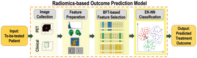
The proposed treatment outcome prediction model.

B. Feature Preparation

We extracted features from image data using a procedure that combines methods outlined in recently published papers [20]. We combined an open-source image processing package (plastimatch) with in-house code developed with MATLAB. About 400 to 600 features are extracted, which include SUV-based, textural and clinical features.

SUV-based features.

For patient cases with longitudinal images, we first registered the in-treatment images acquired at different time points to the pre-treatment PET image via a rigid registration method [21]. Given the metabolic tumor volume (MTV) on PET images of each patient case, we calculate five types of SUV-based features. These features include maximum uptake in MTV (SUVmax), average uptake in MTV (SUVmean), average uptake in the neighborhood of SUVmax (SUVpeak), MTV volume size, and total lesion glycolysis (TLG). We also calculated the temporal changes of these features between the baseline images and the follow-up PET images as additional features [4].

Textural features.

Textural features have been proven to be useful and important for accurate cancer treatment outcome prediction [22]. With the feature extraction package [20], we used the gray-level co-occurrence matrices (GLCMs), gray-level run-length matrices (GLRLMs), and gray level size-zone matrices (GLSZM) to extract texture features [23]. The temporal changes of these features from baseline and the follow-up acquisitions are calculated as additional features.

Clinical features.

Besides the imaging features, we also considered features from other sources of information, including patients clinical characteristics and available genomics expressions, as additional candidate features.

C. BFT-based Predictive Feature Subset Selection

The feature subset selection is achieved through the minimization of a pre-defined loss function, which can be trained with a set of training samples based on Belief-function theory (BFT) [24]. BFT, referred to as evidence theory, is a generalization of both probability theory and set-membership approach. It provides a formal framework for dealing with both imprecise and uncertain data and reasoning under uncertainty based on the modeling of evidence.

1). Mass Function:

Without loss of generality, let $\{X_i,Y_i{\}}_{i=1}^N$ be a data set consisting of N patient samples, $X_i\in {\mathbb{R}}^V$ is the feature vector for the i-th training sample and Y_i ∈ Ω is the corresponding outcome class label. Let Ω = [ω₁, ⋯ , ω_C] be the collection of all possible class labels, and A is a subset of Ω. Based on BFT theory [24], The evidence about the class label of a sample X_i is A can be represented by a mass function m_i (A) defined from the 2^Ω to the interval [0, 1]. m_i (A) represents a degree of belief that supports the actual label of sample X_i in A, and

$$\sum _{A\subseteq \Omega }{m}_i(A)=1.$$ (1)

For any two samples X_i and X_j, the distance d_i,j between X_i and X_j is defined as

$$d_{i,j}=\sqrt{\sum _{v=1}^V{\lambda }_v{d}_{ij,v}^2},$$ (2)

where d_ij,v = ∣x_i,v − x_j,v ∣ represents the difference between the v-th feature of X_i and X_j, 1 ≤ v ≤ V. λ_v can be a binary value 0 or 1 to represent the selection/non-selection of the v-th feature, or performs as a weighting factor to represent the importance of the v-th feature. Let X_j with class label Y_j = ω_c, the mass function provided by X_j for X_i (supports that the label of X_i belongs to ω_c), is defined as

$$\{\begin{array}{cc}{m}_{i,j}(\{{\omega }_c\})\hfill & =e^{-{\gamma }_c{d}_{i,j}^2}\hfill \\ m_{i,j}(\Omega )\hfill & =1-e^{-{\gamma }_c{d}_{i,j}^2}\hfill \end{array}\phantom{\}},$$ (3)

where parameter γ_c is set as the inverse of the mean distance between samples from the same class, and c ∈ C. Large d_i,j represents negligible information provided by the mass function, meaning m_i,j (Ω) ≈ 1. Therefore, the mass functions offered by the first K nearest neighbors of each X_i are sufficient to be used in order to improve the computational efficiency. K = 10 is selected in this study. Let {X_i1 ,…, X_iK} be the selected neighbors for X_i. Correspondingly, {m_i,i1, … , m_i,iK} are the related mass functions. {X_i1, … , X_iK} is then assigned into different groups according to their outcome labels. When C = 2 and ϴ_c ≠ ∅ (c = 1 or 2), the resulting mass function $m_i^{{\Theta }_c}$ can be represented as

$$\{\begin{array}{cc}{m}_i^{{\Theta }_c}(\{{\omega }_c\})\hfill & =1-{\prod }_{X_{i_k\in {\Theta }_c}}^{k=1,\dots ,K}\left(1-e^{-{\gamma }_c{d}_{i,i_k}^2}\right)\hfill \\ m_i^{{\Theta }_c}(\Omega )\hfill & ={\prod }_{X_{i_k\in {\Theta }_c}}^{k=1,\dots ,K}\left(1-e^{-{\gamma }_c{d}_{i,i_k}^2}\right)\hfill \end{array}\phantom{\}},$$ (4)

where $m_i^{{\Theta }_c}(\Omega )=1$ when ϴ_c is empty. A global mass function M_i regarding the class membership of X_i can be calculated as

$$\{\begin{array}{cc}{M}_i(\{{\omega }_1\})\hfill & =m_i^{{\Theta }_1}(\{{\omega }_1\})\cdot m_i^{{\Theta }_2}(\Omega )\hfill \\ M_i(\{{\omega }_2\})\hfill & =m_i^{{\Theta }_2}(\{{\omega }_2\})\cdot m_i^{{\Theta }_1}(\Omega )\hfill \\ M_i(\Omega )\hfill & =m_i^{{\Theta }_1}(\Omega )\cdot m_i^{{\Theta }_2}(\Omega )\hfill \\ M_i(\varnothing )\hfill & =m_i^{{\Theta }_1}(\{{\omega }_1\})\cdot m_i^{{\Theta }_2}(\{{\omega }_2\})\hfill \end{array}\phantom{\}}.$$ (5)

2). Loss Function for Feature Subset Selection:

Based on the global mass function for all training samples to a to-be-tested sample, an loss function is defined for selecting predictive features as a group. Three requirements of the qualified predictive features is considered. First, these features should provide high prediction accuracy. Second, they should yield low uncertainty. Third, they should enable sparsity to reduce over-fitting risk on unseen samples. Considering this, we defined the loss function as

$$L(\Lambda )=(T_1+T_2+\beta \Vert \Lambda \Vert ).$$ (6)

The feature selection is realized by minimizing L(Λ) to find a sparse V dimensional binary vector Λ = {λ₁, λ₂, ⋯ , λ_V}. Λ determines the optimal features of each feature vector X_i as diag(X_iΛ^T) and the v-th feature is selected when λ_v = 1.

T₁ in L(Λ) measures the mean squared error of outcome label estimation accuracy, which supports the hypothesis that the estimated class label ${\widehat{Y}}_i$ is the same as the known label Y_i of the i-th training sample. It is defined as

$$T_1=\frac{1}{N}\sum _{i=1}^N\sum _{c=1}^C\{M_i(\{{\omega }_c\})-Y_{i,c}{\}}^2,$$ (7)

where M_i({ω_c}) is a global mass function regarding the class label of X_i [18], and Y_i,c is the c-th element of the class label, with Y_i,c = 1 if and only if Y_i = ω_c.

T₂ in L(Λ) penalizes features that only provide equal evidences to support the hypothesis that ${\widehat{Y}}_i$ is any class label in Ω, indicating they are non-predictive features and should be ignored. It is defined as

$$T_2=\frac{1}{N}\sum _{i=1}^N(M_i(\varnothing {)}^2+M_i(\Omega {)}^2),$$ (8)

where M_i(∅) denotes the conflict of X_i with its neighborhood, and M_i(Ω) denotes the imprecision of the class label of X_i. The larger M_i(Ω) indicates the higher overlapped area in the feature space that X_i is located. Differently, the larger M_i(∅) indicates the farther away from all other samples.

The last sparsity regularization term $\Vert \Lambda \Vert ={\sum }_{v=1}^V{\lambda }_v$ (the number of nonzero entries in Λ) forces the selected feature subset to be sparse to reduce over-fitting risk on unseen data. The scalar β controls the strength of the sparsity penalty.

The minimization of the loss function is solved by an integer Genetic Algorithm [25], which can achieve the global optima without gradient calculation for non-convex problems.

3). Feature Pre-selection and Data Balancing:

Considering the large number, redundancy and uncertainty of the prepared radiomic features, we pre-determined a number of predictive features from the extracted features before employing the above BFT-based feature selection process. This feature pre-selection procedure can improve the efficiency of the BFT-based feature selection and the stability of the selected feature subsets. Considering 1) the small-sized training samples used in this study and 2) the clinical value of SUV-based features for assessing treatment outcome [26], we incorporated the SUV-based features as pre-defined prior knowledge. In this study, we used a feature ranking method (RELIEF [8]) with a cut-off threshold of 0.9 to pre-select all the extracted features, and required the top-ranked SUV-based features to be included as well.

In addition, the prediction model learned from unbalanced training data might yield high false negative prediction rates on samples belonging to minority class (the class having relatively less number of instances). It might induce the issues of over generalization and variance [27], over-fitting [28], and lose of useful information. We used ADAptive SYNthetic sampling (ADASYN) strategy to over-sample data within the minority class, considering that it can adaptively generate synthetic samples in a data-driven manner [29].

D. Outcome Prediction Based on the Selected Feature Subset

In order to predict treatment outcome, the optimal feature subset selected by the method described in Section II-C should feed into a classifier for outcome prediction. Theoretically, any case-based methods, e.g., K-NN and SVM classifiers, can be used as the classifier. We used a BFT-based classifier, evidential K-NN method [19], [30]–[32] in this study considering its ability of utilizing the imperfect knowledge learned from the training samples for classification.

Let X_i = [x₁, ⋯ , x_V′]^T be the i-th (i ∈ N) training sample with the V′ selected features, where V′ << V, and Y_i ∈ {ω₁, ⋯ , w_C} is the corresponding class label. Given a query instance X^t, its class membership can be determined by the EK-NN method through the following steps. First, each neighbor of X^t is considered as an item of evidence that supports certain hypotheses regarding the class membership of X^t. Let X_j be one of the K nearest neighbors with class label Y_j = ω_c. The mass function induced by X_j, which supports the decision that X^t also belongs to ω_c, is calculated by Eq. 3. The parameters in Eq. 3 is optimized via minimizing a performance criterion constructed on training data. Then, Dempsters rule is performed to combine all neighbors knowledge and obtain a global mass function for X^t. The lower and upper bounds for the belief of any specific hypothesis are then quantified via the credibility and plausibility values, respectively. Corresponding to a normalized mass function m, credibility and plausibility functions Bel(·) and Pl(·) from 2^Ω to [0, 1] are defined as

$$Bel(A)=\sum _{B\subseteq A}{m}_i(B),Pl(A)=\sum _{B\cap A\ne \varnothing }{m}_i(B),$$ (9)

where Bel (A) represents the degree to which the evidence supports the hypothesis ω ∈ A, while Pl(A) represents the degree to which the evidence is not contradictory to that hypothesis. Functions Bel(·) and Pl(·) are linked by the relation $Pl(A)=1-Bel(\overline{A})$ , and in one-to-one correspondence with the mass function m. In the case of {0, 1} losses, the final decision on the class label of X^t can be made alternatively through maximizing the credibility, the plausibility, or the pignistic probability, as defined in the literature [33].

III. Study Population

Clinical data from 25 lung, 36 esophagus, 45 lymphoma, and 63 cervical cancer patient cases were included in the retrospective study. The first three patient cohorts were collected form The Center of Henri-Becquerel (Rouen, France) [34]–[36], while the last patient cohort from Washington University (St. Louis, USA) [37], Details regarding these patient cases are provided in TABLE I.

TABLE I:

Characteristics of four patient cohorts.

Datasets	Recurrence, Disease-positive, Non-complete remission	Non-recurrence, Disease-free, Remission
Stage II-III NSCLC	19	6
ESCC	23	13
Lymph tumor	6	39
Stage II-III Cervical	17	46

Lung Cancer Data.

A cohort of twenty-five patients with inoperable stage II or III non-small cell lung cancer (NSCLC) were collected. These patients are treated with curative-intent chemotherapy or radiotherapy. The total radiation therapy (RT) dose for those patient cases were 60-70 Gy, and has been delivered in daily fractions of 2 Gy and five days a week. Each patient had histological proof of invasive NSCLC. The collected images include a FDG-PET scan at initial staging (i.e., PET₀, the baseline), the first follow-up PET scan (PET₁) obtained after induction chemotherapy and before RT, the second follow-up PET scan (PET₂) obtained during the fifth week of RT (approximately at a total radiation dose of 40-45 Gy). The treatment response was systematically evaluated and followed-up at three months and one year after RT, or if there was a suspicious relapse. Local/distant relapse (LR/DR) vs. complete response (CR) at one year were set as the endpoint. Nineteen LR/DR patients were grouped into the recurrence class (majority class), while the remaining six CR patients were labeled as no-recurrence (minority class). Additional details regarding the patient data can be found in [18], [34].

Esophageal Cancer Data.

A cohort of thirty-six patients with histologically confirmed esophageal squamous cell carcinomas (ESCC), were collected for the study. These patients were treated with definitive three-dimensional conformal RT for a total dose of 50 Gy delivered 2 Gy per fraction. The initial tumor staging was evaluated based on oesophagoscopy with biopsies, PET/CT scans, and endoscopic ultrasonography. Each patient also underwent a FDG-PET/CT scan at initial tumor staging. The patients were evaluated and followed-up for five years. Thirteen patients were grouped to the disease-free class (minority class), since neither locoregional nor distant disease was detected on them. The remaining twenty-three patients were labeled as disease-positive (majority class). Additional details regarding the patient data can be found in [18], [35].

Lymph Cancer Data.

A cohort of forty-five patients with diffuse large B-cell lymphoma (DLBCL), treated with chemotherapy only, were collected as well. For each patient, FDG-PET scans before the chemotherapy and after three/four cycles of chemotherapy were acquired. The treatment response was evaluated according to the International Workshop Criteria (IWC) for non-Hodgkin lymphoma (NHL) response and according to IWC+PET three weeks after the chemotherapy. Thirty-nine patients were grouped to the class of complete remission (majority class); while the remaining six patients with refractory or partial response were grouped to the class of non-complete remission (minority class). More details of this patient cohort is reported in [36].

Cervical Cancer Data.

A cohort of sixty-three patients with stage II or III cervical cancer were collected. Patients were staged clinically according to International Federation of Gynecology and Obstetrics staging. Pre-treatment PET images were used to extract imaging features in the current study. Metabolic tumor volumes (MTVs) were initially defined on diagnostic PET images by SUV thresholding within a suitable region-of-interest followed by manual editing. All patients were treated with concurrent chemotherapy and radiation therapy. Chemotherapy consisted of cisplatin (40 mg/m² weekly for six cycles). Forty-six patients were labeled as non-recurrence (majority class) while the remaining seventeen patients were grouped to the recurrence class (minority class). The radiation treatment was based on standard treatment practices of external intensity-modulated RT irradiation and HDR brachytherapy for cervical cancer at Washington University in St. Louis [37].

IV. Experimental Results

A. Statistical Analysis

We applied the proposed method on the four different patient cohorts. Fifty-two features for lung dataset, 29 features for esophagus dataset, 27 features for lymph dataset, and 73 features for cervix dataset are pre-selected from all extracted features and used as the input of the BFT-based feature selection method. The ADASYN strategy is totally conducted 3 times to deal with the random nature of the data balancing procedure. The optimal feature subset is determined as the most frequently subset that occurred in the three independent runs. The sparsity parameter β was empirically determined by performing extra cross validation on the training set.

Considering the limited number of training samples of these four patient cohorts and for a comprehensive and fair assessment, all the compared methods were evaluated by the .632+ Bootstrapping. The .632+ Bootstrapping can ensure low biased and variable estimation of classification performance on smallsized datasets [38]. At each run of the .632+ Bootstrapping, the training set is a bootstrap generated by sampling from the whole patient cohort, while the testing set consists of the rest of samples in the patient cohort that do not exist in the bootstrap. Statistically, only 63.2% of the original data are used for training in each run. The final evaluation is then determined by combining the average performance of all runs (pessimistically biased estimation) with the performance of training and testing both on the original dataset (optimistically biased estimation). The feature selection stability is defined as the overlap of common selected features for all test patients with all selected features [39]. The prediction performance were assessed with accuracy [40], and receiver operating characteristics (ROC) analysis [41].

B. Discovery of Predictive Features from Patient Cohorts

The most frequent feature subsets selected by the developed model for all four patient cohorts are shown in TABLE II. For the lung patient cohort, the SUVmax during the fifth week of RT (PET₂) and the longitudinal changes of texture features are selected as the predictive radiomic features. Differently, the clinical characteristics (TLG extracted from PET₀ and patient gender) were selected as the predictive features for the esophageal tumor cohort. However, for the cervical cancer patient cohort, the standard deviation of SUVmean and shape/size based features were recognized as the valuable features, while the selected predictive features for the lymph tumor cohort include both longitudinal SUV-based features and genomic features. Although different features were selected for different patient cohorts, these selected predictive features have already been proven to yield predictive power in varied clinical studies [9], [10], [12], [42]. TABLE II demonstrates that in addition to imaging features, other kinds of features are also selected in each subset can give complementary information for these existing measures to improve the prediction performance.

TABLE II:

Selected feature subsets for four patient cohorts

Cohorts	Selected features
Stage II-III NSCLC	SUV-based: SUV max extracted from PET2 GLSZM-based: Gray-level-non-uniformity change between PET2 & PET0 GLSZM-based: change of zone-percentage between PET1 & PET0 GLSZM-based: change of zone-percentage between PET2 & PET0
ESCC	SUV-based: TLG extracted from PET0 Clinical characteristic: Tumor staging as II Clinical characteristic: Patient gender
Lymph tumor	SUV-based: Change of SUV max between PET1 & PET0 SUV-based: SUV max extracted from PET0. Gene expression: MME Gene relates to tumor subtype Gene expression: SLC2A5 Gene relates to glucose transportation
Stage II-III Cervical Cancer	SUV-based: Standard deviation of SUV in tumor volume Shape and Size based: Ratio of surface area to tumor volume GLCM-based: Dissimilarity of gray level co-occurrence matrix GLCM-based: Sum average of gray level co-occurrence matrix GLRLM-based: Run percentage of gray level run-length matrix

C. Performance Comparison with Other Methods

1). Comparison on Feature Selection Stability:

Stability of the selected features is considered as one of the metrics to evaluate the performance of a feature selection method. The comparison on feature selection stability of the proposed method with other nine methods (RELIEF [8], FAST [11], SFS [9], SFFS [9], SVMRFE [10], KCS [12], HFS [42], EFS [43], and the method using all the predetermined features) is shown in Fig. 2. Each feature selection method was optimized based on the strategy proposed in related literature. The value of the feature selection stability ranges from 0 to 1, where 1 means all selected feature subsets are approximately identical for each run of the .632+ Bootstrapping, while 0 represents no intersection among each run. As shown in Fig. 2, the BFT-based method achieves better performance related to feature selection stability than the other methods. The BFT-based method yields the best performance on the cervical patient cohort and the worst on the lymph tumor cohort. Table III shows the numbers of the features selected from all nine methods. The optimal number of the selected features from different methods also varied.

Fig. 2:

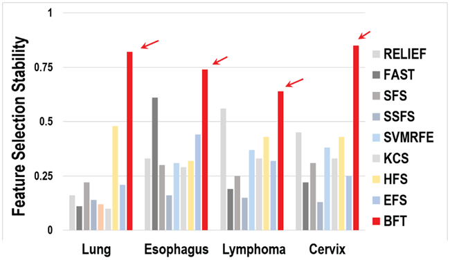
Comparison on feature selection stability.

TABLE III:

The number of selected features.

Methods	Lung	Esophagus	Lymphoma	Cervix
All	52	29	27	73
RELIEF	7	6	4	3
Fast	10	25	15	14
SFS	5	2	1	2
SSFS	5	5	5	5
SVMRFE	5	5	5	5
KCS	29	3	2	38
HFS	3	5	3	7
EFS	4	3	4	5
BFT	4	3	4	5

2). Comparison on Discrimination Power of the Selected Features:

We performed the Andrews plot analysis to compare the discriminative power of the features selected with different methods. An Andrews curve applies the following transformation to each patient dataset,

$$\begin{gathered} f_{X_n}(t)=\frac{X_{n_1}}{\sqrt{2}}+X_{n_2}\sin (t)+X_{n_3}\cos (t) \\ +X_{n_4}\sin (2t)+X_{n_5}\cos (2t)+\cdots , \end{gathered}$$ (10)

where t ranges from 0 to 1 and X_n1, X_n2, ⋯ represent the selected features from each patient dataset X_n. Andrews plot is a graphical data analysis technique for plotting multivariate data, and provides a way to visualize information carried by high-dimensional data [44].

Fig. 3 shows the Andrew plots generated with the selected predictive features from the BFT-based and SVMRFE methods [10] on two patient cohorts of NSCLC and cervical. Blue line represents the curve given the feature input of patients labeled as one type of treatment outcome while orange line represents those of patients labeled as the other treatment outcome. Solid line denotes the median value and dotted line shows the second quartile of the resulted f_Xn (t) from all patient cases. Fig. 3 clearly shows that patients with different treatment outcome can be better stratified by the features selected by the BFT-based method compared to the SVMRFE method. This illustrates that the features selected from the BFT-based method yield more predictive information than those selected by other methods.

Fig. 3:

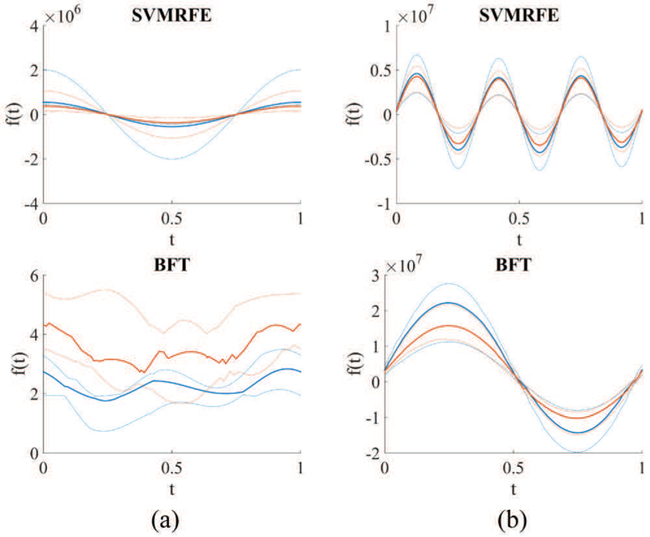
Andrews plot of the selected features by use of the SVMRFE and BFT-based methods on two patient cohorts. (a) Stage II-III NSCLC (b) Stage II-III cervical cancer

D. Comparison on Outcome Prediction Performance

To assess the prediction performance of the BFT-based model, accuracy and AUC metrics were computed for the BFT-based method and other nine methods. The general definition of accuracy and AUC metrics, as that used in [4], [18], are employed in this study too. Fig. 4 shows the prediction performance with EK-NN as the default classifier for all methods. The BFT-based method achieves better results than other methods on all four patient cohorts. The BFT-based model yields lowest prediction accuracy and AUC values on the Esophagus patient cohort compared to the other three cohorts.

Fig. 4:

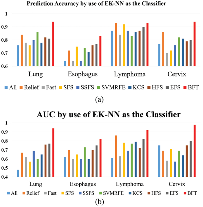
Prediction accuracy and AUC of different feature selection methods with EK-NN used as the classifier. (a) Prediction Accuracy (b) AUC

The method performance by use of EK-NN and SVM as two different classifiers given input the features selected by the BFT-based method was compared as well. The results shown in Fig. 5 demonstrate that combining BFT-based feature selection with the EK-NN classifier can provide higher performance than with other classifiers.

Fig. 5:

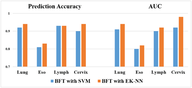
Comparison of using either EK-NN or SVM as the classifier.

E. Effect of Performing Feature Pre-selection

By use of cervical cancer data as an example, we have performed the test by applying BFT-based feature selection method and other nine methods directly on all the extracted features and without performing the feature pre-selection. Here, total of 657 features were extracted for the cervical patient cohort. As shown in Fig. 6, the overall performance of most of the tested methods (including BFT) without performing feature pre-selection is worse than that after performing feature pre-selection (shown in Fig. 4 above). Also, the result achieved by applying the BFT-based method on all features is still slightly better than that from other methods. Performing feature pre-selection improves the prediction performance of the BFT-based method and some other testing methods.

Fig. 6:

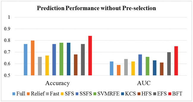
Prediction performance without feature pre-selection.

F. Effect of Performing Data Re-balancing

We evaluated the performance improvement with and without data rebalancing. As shown in Fig. 7, performance is improved on all four patient cohorts by applying data rebalancing. When the dataset is severely imbalanced (e.g., the lung tumor example), the data balancing procedure is especially significant for the improvement of prediction performance.

Fig. 7:

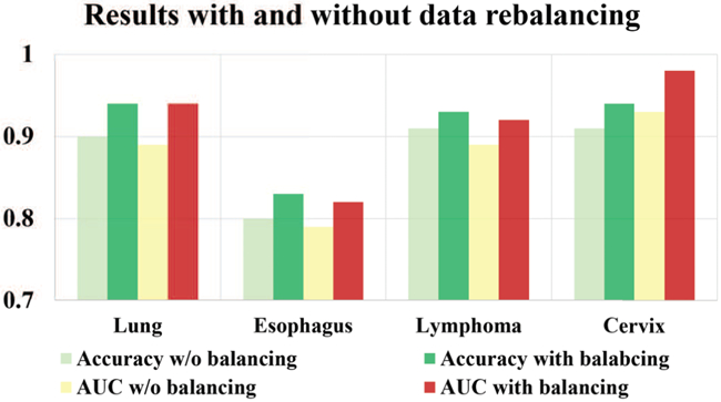
The effect of data re-balancing.

G. Sparsity of the Selected Features

The sparsity term β in the loss function in Eq. 6 plays an important role to find a sparse feature subset which can lead to high prediction accuracy on unseen data. Larger β yields greater sparsity. The number of neighbors, K, in the EK-NN classifier can also affect the prediction performance. We evaluated the prediction performance of the EK-NN classifier with respect to K(1 ≤ K ≤ 10) under different sparsity degree of 0.01, 0.03, and 0.07. Results on NSCLC and cervical patient cohorts are shown in Fig. 8 as two examples. For all four patient cohorts, the BFT-based method consistently leads to better classification performance than using directly all the input features, and also improves the robustness of the EK-NN classifier in terms of parameter K. Also, when β equals 0.03 to 0.07, the proposed method can achieve better classification performance compared to other β across all the studied datasets.

Fig. 8:

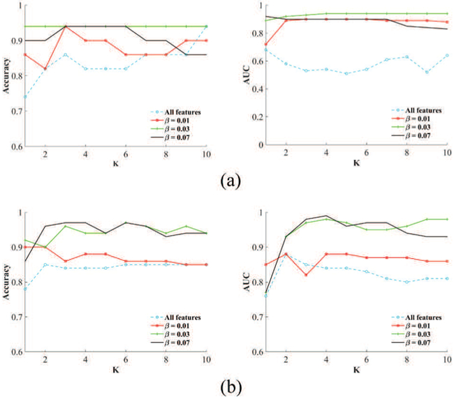
Prediction performance of the EK-NN classifier with respect to different K under different sparsity degrees. (a) NSCLC (b) Stage II-III cervical cancer

H. Computational Complexity

Computational complexity of the BFT-based method mainly depends on the optimization of L(Λ) and the size of input features V. Let O(L) be the computational complexity of calculating loss function L(Λ), O(L) depends on the calculation of T₁, T₂ and ∥Λ∥ in L, which relate to the number of patient data samples N, the number of all possible class labels C, the number of neighbors K for computing mass functions, and the number of input features V. V is much larger than N, C, and K. The computational complexity of the BFT-based method is in the order of O(V).

V. Discussion

A. The Proposed BFT-based Prediction Method

Compared with traditional probability theory that only considers probabilities on individual outcome classes, BFT allows to estimate the probability of the training sample belonging to each individual outcome class and the sets of outcome classes from each feature. The estimations from all features are then combined to a global estimation. Therefore, the uncertainty of the predictive information carried by each feature of each training sample is implicitly integrated into the loss function. The probabilities relating to sets of outcome classes are assigned to each individual class with the pignistic probability transformation and can maximize the final estimation accuracy.

The performance of the BFT-based method on four different patient cohorts was investigated. Different image features were utilized by the prediction method for the different patient cohorts. For the lung patient cohort, radiomic features extracted from pre-, in, and after-treatment PET images were utilized. For cervical cancer patient cohort, only radiomic features extracted from pre-treatment PET images were utilized. Differently, for the esophagus and lymphoma patient cohort, in addition to pre- and post-treatment PET image data, clinical characteristics and genomic features were utilized. As shown in Table II, the most predictive features were selected for different patient cohorts are different. The feature subsets determined by the method are in consistency with the predictors that have been verified in reported clinical studies [9], [10], [12], [42]. It was observed that clinical and genomic features might yield complementary information to radiomic features and potentially improve the prediction performance.

It was also observed that longitudinal features extracted from in- and post-treatment PET images can provide complementary information and improve the prediction performance. Another interesting finding was observed with the cervical patient cohort. Although only pre-treatment PET images were employed for this patient cohort, the feature selection stability and predication performance of the method on this cohort was the best. This might relate to the relatively large size of this patient cohort, but further investigations are needed to confirm this conjecture.

B. Future Work

As shown in Fig. 8, an appropriate control parameter is helpful for the determination of the feature subset. As one of the future work, the strategy to automatically selecting parameters of the model will be investigated. The effect of treatment methodology and treatment dose on prediction performance of tumor control will be investigated as well.

The calculation of some radiomic features depends on the MTV delineation, which might induce some uncertainties in radiomics features. This might affect the model prediction accuracy on patients in different ways. As an interesting future work, two uncertainties will be investigated, including 1) MTV delineation on PET images, (2) limited accuracy of the affine transformations used to map MTVs from PET to other images. Radiomic features calculated from different MTV subregions might yield different prediction accuracy and additional features might affect predictive accuracy compared to that calculated on the whole MTV. The MTV will be separated into a set of sub-regions and calculate features for each subregion.

Multi-modality radiomic features derived from PET, CT, and MR imaging have individually been reported as predictive biomarkers [3], [45], [46]. However, very little research has focused on developing an integrated prediction model to seamlessly fuse the predictive information carried by multimodal features for more accurate outcome prediction. BFT enables various fusion rules to combine predictive information represented by multi-source radiomic features to achieve more accurate prediction (classification) [47]–[50]. The performance improvement by use of multi-modality features in comparison to each single modality will be investigated, and the importance of each modality images will be validated. In addition, the importance of features extracted from images acquired at different time points throughout the treatment will be validated as another future work.

VI. Conclusions

The current study shows that PET-based radiomic features are associated with local tumor control in cancers. As an integrated framework to extract, process, select, and learn from radiomic features, the developed prediction model can provide a complete strategy to improve the accuracy and stability of outcome prediction, and ultimately cancer patient care. The model will guide patient-specific treatment by identifying patients for whom conventional treatment will likely fail as well as people who are candidates for de-escalated treatment with associated reduced normal tissue toxicity.

References

- [1].Ferlay J, Steliarova-Foucher E, Lortet-Tieulent J, Rosso S, Coebergh J-WW, Comber H, Forman D, and Bray F, “Cancer incidence and mortality patterns in europe: estimates for 40 countries in 2012,” European journal of cancer, vol. 49, no. 6, pp. 1374–1403, 2013. [DOI] [PubMed] [Google Scholar]
- [2].Kourou K, Exarchos TP, Exarchos KP, Karamouzis MV, and Fotiadis DI, “Machine learning applications in cancer prognosis and prediction,” Computational and structural biotechnology journal, vol. 13, pp. 8–17, 2015. [DOI] [PMC free article] [PubMed] [Google Scholar]
- [3].Gillies RJ, Kinahan PE, and Hricak H, “Radiomics: images are more than pictures, they are data,” Radiology, vol. 278, no. 2, pp. 563–577, 2015. [DOI] [PMC free article] [PubMed] [Google Scholar]
- [4].Lian C, Ruan S, Denrnux T, Jardin F, and Vera P, “Selecting radiomic features from fdg-pet images for cancer treatment outcome prediction,” Medical image analysis, vol. 32, pp. 257–268, 2016. [DOI] [PubMed] [Google Scholar]
- [5].Cook GJ, Siddique M, Taylor BP, Yip C, Chicklore S, and Goh V, “Radiomics in pet: principles and applications,” Clinical and Translational Imaging, vol. 2, no. 3, pp. 269–276, 2014. [Google Scholar]
- [6].Vallières M, Freeman CR, Skamene SR, and El Naqa I, “A radiomics model from joint fdg-pet and mri texture features for the prediction of lung metastases in soft-tissue sarcomas of the extremities,” Physics in Medicine & Biology, vol. 60, no. 14, p. 5471, 2015. [DOI] [PubMed] [Google Scholar]
- [7].Kumar V, Gu Y, Basu S, Berglund A, Eschrich SA, Schabath MB, Forster K, Aerts HJ, Dekker A, Fenstermacher D et al. , “Radiomics: the process and the challenges,” Magnetic resonance imaging, vol. 30, no. 9, pp. 1234–1248, 2012. [DOI] [PMC free article] [PubMed] [Google Scholar]
- [8].Kira K and Rendell LA, “The feature selection problem: Traditional methods and a new algorithm,” in Aaai, vol. 2, 1992, pp. 129–134. [Google Scholar]
- [9].Pudil P, Novovičová J, and Kittler J, “Floating search methods in feature selection,” Pattern recognition letters, vol. 15, no. 11, pp. 1119–1125, 1994. [Google Scholar]
- [10].Guyon I, Weston J, Barnhill S, and Vapnik V, “Gene selection for cancer classification using support vector machines,” Machine learning, vol. 46, no. 1-3, pp. 389–422, 2002. [Google Scholar]
- [11].Chen X and Wasikowski M, “Fast: a roc-based feature selection metric for small samples and imbalanced data classification problems,” in Proceedings of the 14th ACM SIGKDD international conference on Knowledge discovery and data mining ACM, 2008, pp. 124–132. [Google Scholar]
- [12].Wang L, “Feature selection with kernel class separability,” IEEE Transactions on Pattern Analysis and Machine Intelligence, vol. 30, no. 9, 2008. [DOI] [PubMed] [Google Scholar]
- [13].Ma S and Huang J, “Penalized feature selection and classification in bioinformatics,” Briefings in bioinformatics, vol. 9, no. 5, pp. 392–403, 2008. [DOI] [PMC free article] [PubMed] [Google Scholar]
- [14].Zhou Y, Jin R, and Hoi SC-H, “Exclusive lasso for multi-task feature selection,” in Proceedings of the Thirteenth International Conference on Artificial Intelligence and Statistics, 2010, pp. 988–995. [Google Scholar]
- [15].Cheeseman JKP, Self M and Stutz J, “yesian classification,” 1996. [Google Scholar]
- [16].Ruan D, Intelligent hybrid systems: fuzzy logic, neural networks, and genetic algorithms. Springer Science & Business Media, 2012. [Google Scholar]
- [17].Barber D, Bayesian reasoning and machine learning. Cambridge University Press, 2012. [Google Scholar]
- [18].Lian C, Ruan S, Denœux T, Li H, and Vera P, “Robust cancer treatment outcome prediction dealing with small-sized and imbalanced data from fdg-pet images,” in International Conference on medical image computing and computer-assisted intervention Springer, 2016, pp. 61–69. [Google Scholar]
- [19].Denoeux T, “A k-nearest neighbor classification rule based on dempster-shafer theory,” IEEE transactions on systems, man, and cybernetics, vol. 25, no. 5, pp. 804–813, 1995. [Google Scholar]
- [20].Aerts HJ, Velazquez ER, Leijenaar RT, Parmar C, Grossmann P, Carvalho S, Bussink J, Monshouwer R, Haibe-Kains B, Rietveld D et al. , “Decoding tumour phenotype by noninvasive imaging using a quantitative radiomics approach,” Nature communications, vol. 5, p. 4006, 2014. [DOI] [PMC free article] [PubMed] [Google Scholar]
- [21].Pluim JP, Maintz JA, and Viergever MA, “Mutual-information-based registration of medical images: a survey,” IEEE transactions on medical imaging, vol. 22, no. 8, pp. 986–1004, 2003. [DOI] [PubMed] [Google Scholar]
- [22].Tixier F, Le Rest CC, Hatt M, Albarghach N, Pradier O, Metges J-P, Corcos L, and Visvikis D, “Intratumor heterogeneity characterized by textural features on baseline 18f-fdg pet images predicts response to concomitant radiochemotherapy in esophageal cancer,” Journal of Nuclear Medicine, vol. 52, no. 3, pp. 369–378, 2011. [DOI] [PMC free article] [PubMed] [Google Scholar]
- [23].Thibault G, Angulo J, and Meyer F, “Advanced statistical matrices for texture characterization: application to cell classification,” IEEE Transactions on Biomedical Engineering, vol. 61, no. 3, pp. 630–637, 2014. [DOI] [PubMed] [Google Scholar]
- [24].Shafer G, A mathematical theory of evidence. Princeton university press, 1976, vol. 42. [Google Scholar]
- [25].Damousis IG, Bakirtzis AG, and Dokopoulos PS, “A solution to the unit-commitment problem using integer-coded genetic algorithm,” IEEE Transactions on Power systems, vol. 19, no. 2, pp. 1165–1172, 2004. [Google Scholar]
- [26].Kim R, Ock C, Keam B, Kim TM, Kim JH, Paeng JC, Kwon SK, Hah JH, Kwon T-K, Kim D-W et al. , “Predictive and prognostic value of pet/ct imaging post-chemoradiotherapy and clinical decision-making consequences in locally advanced head & neck squamous cell carcinoma: a retrospective study,” BMC cancer, vol. 16, no. 1, p. 116, 2016. [DOI] [PMC free article] [PubMed] [Google Scholar]
- [27].Chawla NV, Bowyer KW, Hall LO, and Kegelmeyer WP, “Smote: synthetic minority over-sampling technique,” Journal of artificial intel-ligence research, vol. 16, pp. 321–357, 2002. [Google Scholar]
- [28].Batista GE, Prati RC, and Monard MC, “A study of the behavior of several methods for balancing machine learning training data,” ACM SIGKDD explorations newsletter, vol. 6, no. 1, pp. 20–29, 2004. [Google Scholar]
- [29].He H and Garcia EA, “Learning from imbalanced data,” IEEE Transactions on knowledge and data engineering, vol. 21, no. 9, pp. 1263–1284, 2009. [Google Scholar]
- [30].Su Z, Denoeux T, Hao Y, and Zhao M, “Evidential k-nn classification with enhanced performance via optimizing a class of parametric conjunctive t-rules,” Knowledge-Based Systems, 2017. [Google Scholar]
- [31].Liu Z, Pan Q, Dezert J, and Mercier G, “Hybrid classification system for uncertain data,” IEEE Transactions on Systems, Man, and Cybernetics: Systems, vol. 47, no. 10, pp. 2783–2790, 2017. [Google Scholar]
- [32].Liu Z, Pan Q, Dezert J, and Martin A, “Combination of classifiers with optimal weight based on evidential reasoning,” IEEE Transactions on Fuzzy Systems, 2017. [Google Scholar]
- [33].Smets P and Kennes R, “The transferable belief model,” Artificial intelligence, vol. 66, no. 2, pp. 191–234, 1994. [Google Scholar]
- [34].Calais J, Thureau S, Dubray B, Modzelewski R, Thiberville L, Gardin I, and Vera P, “Areas of high 18f-fdg uptake on preradiotherapy pet/ct identify preferential sites of local relapse after chemoradiotherapy for non-small cell lung cancer,” Journal of nuclear medicine, vol. 56, no. 2, pp. 196–203, 2015. [DOI] [PubMed] [Google Scholar]
- [35].Lemarignier C, Di Fiore F, Marre C, Hapdey S, Modzelewski R, Gouel P, Michel P, Dubray B, and Vera P, “Pretreatment metabolic tumour volume is predictive of disease-free survival and overall survival in patients with oesophageal squamous cell carcinoma,” European journal of nuclear medicine and molecular imaging, vol. 41, no. 11, pp. 2008–2016, 2014. [DOI] [PubMed] [Google Scholar]
- [36].Lanic H, Mareschal S, Mechken F, Picquenot J-M, Cornic M, Maingonnat C, Bertrand P, Clatot F, Bohers E, Stamatoullas A et al. , “Interim positron emission tomography scan associated with international prognostic index and germinal center b cell-like signature as prognostic index in diffuse large b-cell lymphoma,” Leukemia & lymphoma, vol. 53, no. 1, pp. 34–42, 2012. [DOI] [PubMed] [Google Scholar]
- [37].Macdonald D, Lin L, Wahab S, Esthappan J, Mutic S, Nantz R, Zoberi I, and Grigsby P, “74: Combined imrt and brachytherapy in the treatment of intact cervical cancer,” International Journal of Radiation Oncology Biology Physics, vol. 66, no. 3, p. S43, 2006. [Google Scholar]
- [38].Efron B and Tibshirani R, “Improvements on cross-validation: the 632+ bootstrap method,” Journal of the American Statistical Association, vol. 92, no. 438, pp. 548–560, 1997. [Google Scholar]
- [39].Somol P and Novovicova J, “Evaluating stability and comparing output of feature selectors that optimize feature subset cardinality,” IEEE Transactions on Pattern Analysis and Machine Intelligence, vol. 32, no. 11, pp. 1921–1939, 2010. [DOI] [PubMed] [Google Scholar]
- [40].Baldi P, Brunak S, Chauvin Y, Andersen CA, and Nielsen H, “Assessing the accuracy of prediction algorithms for classification: an overview,” Bioinformatics, vol. 16, no. 5, pp. 412–424, 2000. [DOI] [PubMed] [Google Scholar]
- [41].Hanley JA, “Receiver operating characteristic (roc) curves,” Encyclopedia of biostatistics, 1998. [Google Scholar]
- [42].Mi H, Petitjean C, Dubray B, Vera P, and Ruan S, “Robust feature selection to predict tumor treatment outcome,” Artificial intelligence in medicine, vol. 64, no. 3, pp. 195–204, 2015. [DOI] [PubMed] [Google Scholar]
- [43].Lian C, Ruan S, Denœux T, Li H, and Vera P, “Dempster-shafer theory based feature selection with sparse constraint for outcome predic-tion in cancer therapy,” in International Conference on Medical Image Computing and Computer-Assisted Intervention Springer, 2015, pp. 695–702. [Google Scholar]
- [44].Andrews DF, “Plots of high-dimensional data,” Biometrics, pp. 125–136, 1972. [Google Scholar]
- [45].Aerts H, “Radiomics: there is more than meets the eye in medical imaging (conference presentation),” in SPIE Medical Imaging International Society for Optics and Photonics, 2016, pp. 97 850O–97 850O. [Google Scholar]
- [46].Lambin P, Rios-Velazquez E, Leijenaar R, Carvalho S, van Stiphout RG, Granton P, Zegers CM, Gillies R, Boellard R, Dekker A et al. , “Radiomics: extracting more information from medical images using advanced feature analysis,” European journal of cancer, vol. 48, no. 4, pp. 441–446, 2012. [DOI] [PMC free article] [PubMed] [Google Scholar]
- [47].Trabelsi A, Elouedi Z, and Lefèvre E, “Belief function combination: comparative study within the classifier fusion framework,” in The 1st In-ternational Conference on Advanced Intelligent System and Informatics (AISI2015), November 28–30, 2015, Beni Suef, Egypt Springer, 2016, pp. 425–435. [Google Scholar]
- [48].Murphy RR, “Dempster-shafer theory for sensor fusion in autonomous mobile robots,” IEEE Transactions on Robotics and Automation, vol. 14, no. 2, pp. 197–206, 1998. [Google Scholar]
- [49].Lian C, Ruan S, and Denœux T, “An evidential classifier based on feature selection and two-step classification strategy,” Pattern Recognition, vol. 48, no. 7, pp. 2318–2327, 2015. [Google Scholar]
- [50].Denœux T, “Conjunctive and disjunctive combination of belief functions induced by nondistinct bodies of evidence,” Artificial Intelligence, vol. 172, no. 2-3, pp. 234–264, 2008. [Google Scholar]