Ultrafast two-photon imaging of a high-gain voltage indicator in awake behaving mice

SUMMARY

Optical interrogation of voltage in deep brain locations with cellular resolution would be immensely useful for understanding how neuronal circuits process information. Here, we report ASAP3, a genetically encoded voltage indicator with 51% fluorescence modulation by physiological voltages, sub-millisecond activation kinetics, and full responsivity under two-photon excitation. We also introduce an ultrafast local volume excitation (ULoVE) method for kilohertz-rate two-photon sampling in vivo with increased stability and sensitivity. Combining a soma-targeted ASAP3 variant and ULoVE, we show single-trial tracking of spikes and subthreshold events for minutes in deep locations, with subcellular resolution, and with repeated sampling over days. In the visual cortex, we use soma-targeted ASAP3 to illustrate cell type-dependent subthreshold modulation by locomotion. Thus, ASAP3 and ULoVE enable high-speed optical recording of electrical activity in genetically defined neurons at deep locations during awake behavior.

ETOC

The genetically encoded voltage indicator, ASAP3, provides improved voltage responses and activation kinetics that enables single-trial tracking of action potentials and subthreshold events with subcellular resolution deep in the mouse brain during behavioral tasks when imaged with ULoVE, a kilohertz-rate two-photon sampling method with increased stability and sensitivity.

Graphical Abstract

INTRODUCTION

The ability to optically record electrical activity in individual genetically labeled neurons within behaving animals would greatly facilitate efforts to understand how nervous systems process information (Lee et al., 2006). Fluorescent genetically encoded voltage indicators (GEVIs) can reveal non-spiking electrical activity and resolve action potential (AP) timing with sub-millisecond resolution, tasks that cannot be performed by fluorescent genetically encoded calcium indicators (GECIs) (Lin and Schnitzer, 2016). Multi-photon microscopy, by selectively exciting fluorescence only within a focal point, suppresses the generation of background fluorescence and enables segregation of signals between cells at deeper locations than one-photon microscopy, and thus has been essential for imaging GECIs in many regions of the brain (Svoboda and Yasuda, 2006).

The unique capabilities of GEVIs and multi-photon microscopy, however, have yet to be combined for single-trial voltage recordings in individual neurons within the mammalian brain. Indeed, fast multi-photon voltage recording has been considered exceedingly difficult or impractical. Multi-photon recording of GECIs is typically performed by raster scanning an entire plane at sampling rates of ≤ 30 Hz, suitable for detecting calcium transients which persist for hundreds of milliseconds. However, GEVIs that are fast enough to track APs, which persist for only a few milliseconds, would require sampling rates 1–2 orders of magnitude faster. If raster scanning were sped up, then laser power would need to be increased to maintain photon flux per voxel. Furthermore, as GEVIs reside in the membrane rather than the cytosol, the number of GEVI molecules in an optical section is typically less than for GECIs, reducing the integrated signal per neuron (Brinks et al., 2015; Sjulson and Miesenbock, 2007). These considerations have led to predictions that extremely high illumination powers would be required for multi-photon voltage imaging, leading to rapid photodamage and photobleaching (Brinks et al., 2015; Kulkarni and Miller, 2017)

Given these constraints, the development of GEVIs with large responses and optimized kinetics is crucial for maximizing the chance of detecting electrical events in neurons. Currently, the GEVIs with the largest responses to both subthreshold changes and APs are based on two types of voltage-sensing domains: seven-transmembrane helix opsins and four-transmembrane helix voltage-sensing domains (VSDs). Opsin-based GEVIs have been used in vivo with one-photon excitation to report electrical activity of superficially located neurons (Gong et al., 2015; Lou et al., 2016), but their responsivity is severely attenuated under two-photon excitation (Brinks et al., 2015; Chamberland et al., 2017). In contrast, ASAP-family GEVIs, composed of a circularly permuted green fluorescent protein variant inserted within the fourth transmembrane helix VSD of G. gallus voltage-sensing phosphatase (Figure 1a), are fully responsive under two-photon excitation (Brinks et al., 2015; Chamberland et al., 2017). In particular, ASAP2s demonstrates the largest response per AP of fluorescent protein-based GEVIs, although its kinetics are slower than earlier ASAP variants (Chamberland et al., 2017).

Figure 1. Electroporation-based screening of GEVIs.

(A) Left, responses of various GEVIs in HEK293-Kir2.1 cells to a 0.01-ms 150-V pulse recorded at 100 Hz. ASAPIncp is a voltage-insensitive variant of ASAP1 in which the GFP was de-permuted (Chamberland et al., 2017). Solid traces, mean responses. Data are from five or six wells from two separate experiments, with the top five responders in each well analyzed. Right, fluorescence responses were recorded at 200 Hz in HEK293A cells expressing various GEVIs in response to a voltage step from −70 to 0 mV (ASAP1ncp, n = 4; ASAP1, n = 6; Arclight, n = 3; ASAP2s, n = 10). Error bars, standard deviation (SD). (B) ASAP can be directly expressed from these unpurified PCR products. HEK293-Kir2.1 cells were transiently transfected using Lipofectamine 3000 and either pc3-CMV-ASAP2s plasmid or linear ASAP2s product generated by PCR. Intensity scaling is the same across images. (C) Overview of the screening system. HEK293-Kir2.1 cells expressing GEVI variants are plated in 384-well plates on conductive glass slides connected to a square-pulse generator. The medium in each well is sequentially contacted by a motorized platinum electrode during imagine by a high-speed CMOS camera. The entire procedure is automated by MATLAB routines. (D) Left, model of ASAP domain organization. Right, residues targeted for mutagenesis in the S3-cpGFP linker. (E) Evolutionary history of ASAP3. (F) Fluorescence responses from the third round of electrical screening for the parental ASAP2f L146G S147T R414Q (left) and the best performing mutant, ASAP2f L146G S147T S150G H151D R414Q (right). (G) One-photon fluorescence response curves of ArcLight Q239 (n = 3), ASAP2f R414Q (n = 6), and ASAP3 (n = 10) from HEK293 cells stepped for 500ms from a holding potential of −70 mV. See also Figures S1–S4.

Here we report the identification of an improved indicator, ASAP3, from rapid library generation and electrical screening in mammalian cells. ASAP3 features the largest response among brightly fluorescent GEVIs to either steady-state voltages or APs under either one- or two-photon excitation, favorable kinetics for both AP timing and detection, and efficient membrane localization. In addition, we introduce an Ultrafast Local Volume Excitation (ULoVE) strategy for two-photon microscopy to selectively excite large membrane areas at sampling rates of up to 15 kHz per cell. Applying soma-localized ASAP3-Kv and ULoVE two-photon microscopy in awake head-fixed mice, we detect APs and subthreshold voltage dynamics of cortical and hippocampal neurons in single trials, with sub-millisecond temporal resolution, over durations of minutes, and across multiple days. Finally, we use ASAP3-Kv and ULoVE to illustrate cell type-specific modulation of subthreshold voltage by locomotion in the visual cortex.

RESULTS

An electroporation-based screen for improved GEVIs

Screening for GEVI improvements has been hindered by the lack of rapid and reliable methods to impose known membrane potentials as cells are imaged. We hypothesized that electroporation could serve as a high-throughput method for changing membrane potential. Indeed, we found that ASAP1 transiently expressed in HEK293-Kir2.1 cells responded to electroporation with the expected fluorescence dimming (Figures 1A, S1A–S1C). Further validating this method, we found that ASAP1 and ArcLight responses to electroporation matched those to voltage steps from −70 to 0 mV under voltage clamp electrophysiology (Figure 1A and Table 1). As expected from its faster kinetics, ASAP1 responses reached steady state more quickly than ArcLight (Table S1).

Table 1.

Characteristics of GEVIs used for single-trial imaging in mammalian brain

	ArcLight Q239a	Ace2N-4aa-mNeonb	Archon1c	Quasar2/3d	ASAP2se	ASAP3e
Molar brightnessf
At −70 mV (mM−1 cm−1)	22	≤ 90	∼0.076	∼0.027	ND	15
At +30 mV (mM−1 cm−1)	14	≤ 74	∼0.14	∼0.038	ND	7.5
Activation kinetics at 22–23 °C
Fast time constant (Tfast)	28 ms	0.37 ± 0.08 ms	∼5.2 ms	∼3.3 ms	7.0 ± 0.1 ms	3.7 ± 0.1 ms
Fast component amplitude	39%	58 ± 5%	ND	ND	77 ± 3%	81 ± 1%
Slow time constant (Tslow)	271 ms	5.5 ± 1.4 ms	ND	ND	79 ± 4 ms	48 ± 4 ms
Deactivation kinetics at 22–23 °C
Fast time constant (Tfast)	104 ms	0.50 ± 0.09 ms	∼2.4 ms	∼0.89 ms	16.7 ± 0.3 ms	16.0 ± 0.3 ms
Fast component amplitude	61%	60 ± 6%	ND	ND	65 ± 4%	81 ± 1%
Slow time constant (Tslow)	283 ms	5.9 ± 0.9 ms	ND	ND	116 ± 11 ms	102 ± 2 ms
Activation kinetics at 32–35 °C
Fast time constant (Tfast)	9 ± 1 ms	2.2 ± 0.02 ms	0.61 ± 0.02 ms	0.9 ± 0.06 ms	1.50 ± 0.13 ms	0.94 ± 0.06 ms
Fast component amplitude	50 ± 3%	61%	88%	67%	67 ± 2%	72 ± 1%
Slow time constant (Tslow)	48 ± 4 ms	6.4 ± 0.02 ms	8.1 ± 0.02 ms	11.7 ± 0.2 ms	7.80 ± 0.41 ms	7.24 ± 0.38 ms
Deactivation kinetics at 32–35 °C
Fast time constant (Tfast)	17 ± 1 ms	3.8 ± 0.02 ms	1.1 ± 0.1 ms	1.6 ± 0.1 ms	3.40 ± 0.37 ms	3.79 ± 0.15 ms
Fast component amplitude	79 ± 3%	90%	88%	76%	63 ± 9%	76 ± 5%
Slow time constant (Tslow)	60 ± 7 ms	17.5 ± 0.2 ms	13 ± 1 ms	20 ± 2 ms	13.10 ± 2.11 ms	16.00 ± 1.21 ms
Voltage-responsivity (1-photon)g
ΔF/F per 100-mV step	∼35%	∼−9%	81 ± 3%	46 ± 2%	−36 ± 2%	−51 ± 1 %
ΔF/F per single AP	−3.2 ± 2.2%	∼−5%	30 ± 2%	ND	−7 ± 1%	−18 ± 1%
Voltage-responsive under 2-photon	Yes	No	No	No	Yes	Yes

GEVIs with demonstrated utility in single-trial recordings in mammalian neurons in brain slices or living animals are included for comparison. For standardized comparisons across studies, kinetics measured in mammalian cells in response to step voltages from a −80 or −70 mV baseline to +20 or +30 mV, and AP responses measured in cultured rat hippocampal neurons with a sampling rate of 1–2 kHz, are listed. Responses had reached steady state before voltage was returned to baseline for measurement of deactivation kinetics. Values are mean ± SEM.

^aValues from Jin et al., 2012, with n = 6 HEK293 cells for kinetics and 20 neurons for APs, except for kinetic parameters at 22–23°C, which are from Zou et al., 2014.

^bValues from Gong et al., 2015, except for kinetic parameters at 32–35°C from Piatkevich et al., 2018. For kinetics at 22–23°C, n = 6 HEK293 cells. For kinetics at 32–35°C, n = 17 neurons, with reported SD values converted to SEM.

^cValues from Piatkevich et al., 2018, with time constants at 22–23°C converted from reported t-half values, and with brightness calculated from the estimated brightness of Archer (Lin and Schnitzer, 2016) and the relative brightness of Archon1. For kinetics and single APs, n = 10 neurons. For 100-mV steps, n = 6 HEK293 cells. Reported SD values were converted to SEM.

^dValues are from Piatkevich et al., 2018, and measured on Quasar2, with time constants at 22–23°C converted from reported t-half values, and with brightness calculated from the estimated brightness of Archer (Lin and Schnitzer, 2016) and the relative brightness of Quasar2. For kinetics, n = 11 neurons. For 100-mV steps, n = 5 HEK293 cells. Reported SD values were converted to SEM. Note Quasar3 is equivalent to Quasar2 with an intracellular loop mutation and appended trafficking signals for improved membrane localization. The common parameters measured for both Quasar3 in Adam et al., 2019 and Quasar2 in Piatkevich et al., 2018 (kinetics at 33°C and ΔF/F per 100-mV step at 22°C) were within measurement error between the two studies.

^eFrom this study. For kinetic and steady-state measurements at 22°C, 9 or 10 HEK293 cells expressing ASAP2s or ASAP3, respectively, were patch-clamped. For kinetic and steady-state measurements at 33°C, 7 or 16 CHO cells expressing ASAP2s or ASAP3, respectively, were patch-clamped. For AP responses, 4 or 5 neurons were patch-clamped. Brightness values of ASAP3 were calculated by comparison to a construct in which EGFP replaced the cpGFP in ASAP3, normalized for expression by a fused RFP.

^fAt peak excitation wavelength for fluorescent protein-containing GEVIs or 633 nm for opsin-only GEVIs.

^gMeasurements obtained at 22–23°C except for ΔF/F per single AP of Archon1.

We expressed GEVI variants in cells by transfection in multi-well plates, as possession of the GEVI gene prior to its expression removes the need to retrieve cells after screening. The large number of cells imaged for each mutant also improves performance assessment. To speed up GEVI construction and expression, we devised a protocol for PCR construction of full-length genes and direct transfection of PCR products (Figures 1B, S1D–S1F). In contrast, other GEVI screens utilize plasmid transfection, which introduces the costly and time-consuming steps of plasmid assembly, transformation, picking, culturing, and purification (Abdelfattah et al., 2016; Hochbaum et al., 2014; Piatkevich et al., 2018; Platisa et al., 2017; Tsutsui et al., 2014). Second, unlike other GEVI screens, we produced all mutants deterministically, e.g. mutating two sites to all 400 possible amino-acid combinations. This eliminated the need for oversampling to account for Poisson distributions, further improving screening efficiency. Finally, we devised MATLAB routines to perform electroporation, image capture, and image analysis (Figures 1C, S1G, and S1H). This successfully distinguished sensors with distinct responsivity and kinetics (Figure S1I. Automated screening and analysis enabled the evaluation of thousands of mutants daily, two orders of magnitude faster than patch-clamp electrophysiology.

Mechanism-based evolution of ASAP3

To generate an optimal ASAP-family template for mutagenesis and library-based screening, we first explored combining known beneficial mutations. ASAP2f differs from ASAP1 by a shorter S3-cpGFP linker and is more responsive to hyperpolarization (Yang et al., 2016a). ASAP2s differs from ASAP1 by mutation of Arg-415 to Gln (R415Q) and is more responsive to depolarization but reduced in speed (Table 1 and Table S1) (Chamberland et al., 2017). The combined mutant, ASAP2f R414Q (where aa 414 corresponds to aa 415 in ASAP2s), exhibited responsivity similar to ASAP2s and slightly slower kinetics (Figure S2A and S2B and Table S1). This construct was chosen as the mutagenesis template because its shorter S3-cpGFP linker reduces the sequence search space while potentially enabling tighter conformational coupling between the VSD and cpGFP domains.

In GCaMP, deprotonation of the cpGFP chromophore underlies fluorescence enhancement by calcium (Wang et al., 2008). We postulated that voltage also modulates fluorescence by regulating chromophore protonation in ASAP. Specifically, conformational changes in the VSD may be transduced from the S3-cpGFP linker through the first three positions of cpGFP to influence the position of His-151 (His-148 in wild-type GFP), which normally stabilizes the deprotonated (blue-absorbing) state of the chromophore via hydrogen bonding. We thus decided to target amino acids 146–151, beginning in the S3-cpGFP linker and ending at His-151 (Figure 1D), choosing one or two sites for saturation mutagenesis in each round. Over five rounds of screening, four of which involved combinatorial mutagenesis at two positions (Figures 1E, 1F, and S2–S4), we obtained a variant that responded to depolarization from −70 to +30 mV with a fluorescence change (ΔF/F) of −50.9% ± 1.1% (mean ± standard error of the mean (SEM), n = 10 cells). This is the largest fluorescence response among fluorescent protein-based voltage indicators characterized so far, representing a 46% improvement over the −34.9% ± 1% response (n = 6 cells) of ASAP2f R414Q (Figure 1G). We named this variant, which differs from ASAP2f by the mutations L146G S147T N149R S150G H151D R414Q, as ASAP3.

Characterization of ASAP3 in cultured cells

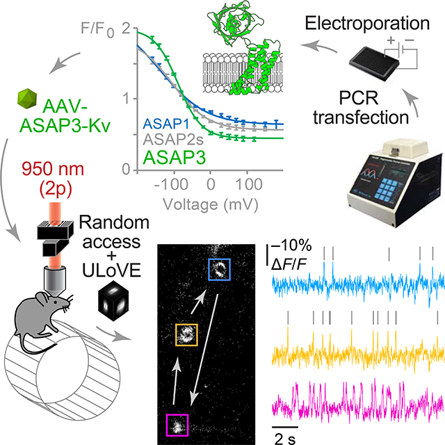
To understand the improved responsiveness of ASAP3, we first analyzed fluorescence-voltage (F-V) relationships. The F-V curves of ASAP1, ASAP2s, and ASAP3 were well fit by sigmoidal Boltzmann functions, similar to gating charge movements of VSDs (Lee and Bezanilla, 2017) (Figure S5A). ASAP3 showed a larger maximal fluorescence change across the extrapolated voltage sensitivity range (4.5-fold) than ASAP2s or ASAP1 (3.3-fold each), due to more complete dimming at positive membrane voltages (Figure S5A). The F-V curves additionally revealed narrowing of the voltage range and progressive right-shifting of the voltage midpoint (V_1/2), from −136 mV in ASAP1 to −104 mV in ASAP2s and −88 mV in ASAP3 (Figure 2A). As these V_1/2 values are all to the left of physiological voltages, narrowing and right-shifting of the voltage input range enhances responsiveness to physiological events.

Figure 2. Characterization of ASAP3 in cells.

(A) Fluorescence-voltage (F-V) curves for ASAP variants. Normalized sigmoid traces fit to steady-state fluorescence responses of ASAP1 (blue trace, n = 6 and 4), ASAP2s (purple, n = 5 and 7), or ASAP3 (green, n = 3 and 6). Error bars, standard error of the mean (SEM). (B) ASAP3 fluorescence activation kinetics during a sustained voltage step from −80 to +20 mV (top) and deactivation kinetics following a 1 ms voltage step from −80 to +20 mV (bottom) in an example CHO cell at 33 °C. Activation kinetics (T_fast = 0.7ms, 72%; T_slow = 4.7ms for this cell) were faster than deactivation kinetics (T_fast = 1.0 ms, 50%; T_si_ow = 4.7ms). (C) Top, fast activation time constant and weighted deactivation time constant during various voltage steps from or to a holding potential of −80 mV, respectively. A single weighted deactivation time constant t was calculated for each potential as (a₁T₁ + a₂T₂)/(a₁ + a₂), where a₁ and a₂ are the coefficients for the bi-exponential fit with time constants t₁ and t₂. Circles and error bars represent mean ± standard deviation (SD) for n = 16 cells. Bottom, fraction of steady-state response achieved by the fluorescence transient evoked by a 1-ms depolarizing pulse. (D) Top, one-photon wide-field image of a representative cultured hippocampal neuron showing efficient plasma membrane localization of ASAP3. Below, response of ASAP3 fluorescence in a dendritic region including spines upon a commanded voltage change from −70 to +30 mV. (E) Responses of ASAP2s and ASAP3 to current-evoked APs in cultured hippocampal neurons with similar AP waveforms (peak amplitudes of 63.5 ± 0.8 mV and 63.7 ± 1.0 mV; full width at half-maximum of 5.0 ± 0.1 and 3.9 ± 0.2 ms for ASAP2s and ASAP3 respectively). Grey lines, single-trial responses (n = 25 each). Colored lines, mean responses. (F) Mean peak fluorescence response, optical spike width at half-maximum, and area under the curve of ASAP2s (n = 4) and ASAP3 (n = 5) in cultured hippocampal neurons. Each neuron fired 3–34 APs, whose values were averaged. (G) Electrical and optical responses from a representative cultured hippocampal neuron expressing ASAP3 in current-clamp mode. Asterisks indicate spontaneous spikes not elicited by current injection. (H) Example voltage (top) and ASAP3 fluorescence (bottom) traces showing ASAP3 responses to sEPSPs of various amplitudes. See also Figure S5.

We next characterized ASAP3 activation kinetics. The ASAP3 response to a 100-mV voltage step at room temperature was well fit to a biexponential curve (Figure S5B), with a fast time constant (T_fast) of 3.7 ± 0.1 ms (mean ± SEM, n = 12 cells), significantly shorter than the 7.0 ± 0.1 ms measured for ASAP2s (Table 1). The amplitude of T_fast was 81 ± 1% for ASAP3, similar to the 77 ± 3% of ASAP2s (Table 1). Responses to hyperpolarization were also faster for ASAP3 than ASAP2s (Table S1). At 33 °C, the response to a 100-mV depolarizing step exhibited a T_fast of 0.94 ± 0.06 ms (mean ± SEM, n = 16 cells) with amplitude of 72 ± 1 %, 1.6-fold faster than ASAP2s (T_fast = 1.50 ± 0.13 ms, amplitude = 67 ± 2%, n = 7 cells) (Figures 2B, 2C, and S5C and Table 1). Thus, ASAP-family kinetics are approximately 4-fold faster at 33 °C than at 22 °C, with ASAP3 exhibiting a sub-millisecond activation time constant. Consistent with its improved kinetics, ASAP3 reached 54 ± 1% (mean ± SEM, n = 16 cells) of its steady-state response within a 1-ms voltage step (Figure 2B and 2C), compared to 39 ± 1% (n = 7 cells) for ASAP2s.

For spike detection, fast activation and delayed deactivation is desirable, as this maximizes the integrated fluorescence change per spike (Wilt et al., 2013) and facilitates template matching for spike identification (Chamberland et al., 2017). Interestingly, ASAP3 retained the relatively slow inactivation kinetics of ASAP2s. Specifically, ASAP3 returned to baseline after a 1-ms depolarizing step with T_fast = 1.48 ± 0.09 ms (mean ± SEM, amplitude 60 ± 3%, n = 16 cells) and T_slow = 6.30 ± 0.40 ms, resulting in an overall weighted deactivation time constant of 3.41 ± 0.21 ms (Figure 2C, Table S1). The corresponding parameters for ASAP2s were T_fast = 2.11 ± 0.40 ms (mean ± SEM, amplitude = 53 ± 10%, n = 7 cells) and T_slow = 7.10 ± 1.62 ms (Table S1).

The 46% larger response to 1-ms steps and 60% faster activation kinetics of ASAP3 vs. ASAP2s should improve spike detection in neurons, as long as expression levels and membrane localization are not impaired. In cultured rat hippocampal neurons, ASAP3 efficiently localized to the plasma membrane (Figure 2D), similar to other ASAP variants (Chamberland et al., 2017; St-Pierre et al., 2014; Yang et al., 2016a). ASAP3 fluorescence outlined dendritic spines, and all cellular ASAP3 signal responded to voltage steps (Figures 2D and Video S1). ASAP3 was also as bright as ASAP2s at rest (Figure S5D). Responses to current-evoked APs (Figure 2E) were 2.7-fold higher with ASAP3 than with ASAP2s (ΔF/F of −17.9 ± 1.2% vs −6.6 ± 0.8% at room temperature), and were also 2.4-fold larger in integrated signal (Figure 2F). Thus, responses to APs are substantially improved with ASAP3 over ASAP2s.

Extended recordings revealed ASAP3 tracking both spikes and subthreshold voltage changes (Figure 2G). We thus examined the sensitivity and linearity of ASAP3 responses to somatically recorded spontaneous excitatory postsynaptic potentials (sEPSPs), defined as transient depolarizing events of 10–100 ms duration (Fricker and Miles, 2000). After applying a 6-pole 50-Hz Bessel filter to the ASAP3 signal to isolate events with these kinetics and remove photon shot noise, we found that sEPSPs correlated with ASAP3 fluctuations in a linear manner in both amplitude (R² = 0.78, conversion factor −0.46% ΔF/F per mV) and duration (R² = 0.72, conversion factor 1.09, Figure S5E). Fluctuations from residual noise in the ASAP3 trace (fluctuations with similar kinetics to sEPSPs but uncorrelated with voltage) were small in magnitude, with root mean square (RMS) of 0.31% ΔF/F, and were rare, occuring once each 610 ms on average in our recordings. By setting a detection threshold at two times the RMS of residual fluctuations, 59% of sEPSPs between 1 and 2 mV and 100% of sEPSPs above 2 mV could be detected (Figure S5E), while limiting the predicted false positive rate to once per 12 s. Sensitivity and linearity for sEPSPs of various amplitudes ≥ 2 mV was confirmed by closer inspection of voltage and fluorescence traces (Figure 2H). Thus, ASAP3, in addition to detecting APs, can also detect sEPSPs with high sensitivity and specificity.

Two-photon responsiveness and soma-targeting of ASAP3 in neuronal tissue

We next characterized ASAP3 responses in neuronal tissue under random-access multiphoton (RAMP) excitation (Figure 3A). In cultured hippocampal slices, ASAP3 activation kept pace with the rising phase of APs, evoked and recorded by patch-clamp electrophysiology, at either 20 °C or ~32 °C (Figure 3B). Inactivation was more prolonged than AP repolarization (Figure 3B), as expected from ASAP3 kinetics (Table 1). ASAP3 produced responses of 17.0 ± 0.8% to single APs at ~32 °C, significantly larger than ASAP2s at 11.7 ± 0.7% (mean ± SEM, n = 12 neurons each) (Figure 3C), and similar to one-photon responses in cultured neurons (Figure 2C and 2D). The discriminability index (d’) (Wilt et al., 2013) for single APs was higher for ASAP3 than AsAp2 (22.5 ± 4.4, n = 3 neurons, vs. 12.2 ± 1.32, n = 11 neurons, recorded at 20 voxels per neuron). With 925-Hz sampling, a d’ value of 22.5 implies a theoretical false positive rate of once per 2.6 × 10²² hours and a false negative probability of 1.2 × 10⁻²⁹ per event.

Figure 3. Spike detection in mammalian brain tissue by ASAP3 and two-photon microscopy.

(A) An overlay image of a two-photon maximum-intensity z projection of an ASAP3-expressing neuron in a cultured hippocampal slice, in the whole-cell configuration with an intracellular solution containing red fluorescent Alexa Fluor 594. The inset shows the expanded somatic region of the neuron, with red dots marking the 20 recorded voxels. (B) Representative examples of ASAP3 optical responses from the neuron in A to current-evoked APs acquired at 20 °C or 32 °C. The ASAP3 signal tracks the rising phase of AP, but exhibits a longer decay time than the AP. About half of the decay kinetics are accounted for by a time constant of 4.3 ± 0.4 ms (n = 12 neurons) at 32 °C or 9.3 ± 1.9 ms (n = 8) at 20 °C. A second component of about 30 ms accounted for the other half of the decay, which may relate to the decay of the underlying after-depolarization. (C) Left, representative examples of ASAP2s and ASAP3 responses to current-evoked APs acquired from cells in cultured hippocampal slices at 32 °C (ave rage of 20 voxels over 10 trials). Right, ASAP3 shows higher peak amplitude responses than ASAP2s to current-evoked APs recorded at 32 °C ***p < 0.0001 (two-tailed t-test). Bars represent mean ± SEM. (D) Left, schematic of whole cell current-clamp and ULoVE recordings of molecular layer interneurons in a parasagittal cerebellar slice expressing ASAP3-Kv. Right, two-photon stack projection of sparse ASAP3 expression in molecular layer interneurons in a parasagittal cerebellar slice. The inset shows the expanded somatic region of the neuron, with red ellipsoids marking the regions of optical acquisition. (E) Left, averaged ASAP3 fluorescence transient (50 trials) for the interneuron in G shows a characteristic interneuron waveform with after-hyperpolarization. Right, ASAP3 shows improved responsivity over ASAP2s for APs in molecular layer interneurons. Bars represent mean ± SEM. *p = 0.026 (Wilcoxon rank sum test). (F) Representative projection confocal images of ASAP3 (left) and ASAP3-Kv (right) expression in cortical slices reveal that the Kv2.1 PRC motif enriches ASAP3 signals in cell soma. (G) Schematic of whole cell current-clamp and optical line-scan recordings of ASAP3-Kv from medium spiny neurons in acute striatal slice. (H) ASAP3-Kv fluorescence reliably tracks 10-Hz (left) or 100-Hz (right) current-evoked AP trains in acute slices. A single unfiltered trace is shown. See also Figure S6.

To challenge ASAP3 in a difficult task, we patch-clamped molecular layer interneurons in acute cerebellar slices while monitoring ASAP3 signal with RAMP microscopy (Figure 3D). At 34 °C, these neurons generate very narrow spikes with full width at half maximum of 0.43 ± 0.06 ms (mean ± SD, Figure 3E). ASAP3 still produced ΔF/F of 8.3% ± 1.1% (mean ± s.e.m. n = 6 neurons), outperforming the 5.3 ± 0.9% of ASAP2s (n = 5 neurons, Figure 3E). These results further confirm that ASAP3 outperforms ASAP2s under two-photon microscopy.

To perform optical voltage recordings in densely labelled tissue, it is useful to remove GEVI signal from neurites, whose diffuse distributions prevent the isolation of signals from individual cell bodies. We had previously concentrated ASAP2s signal in neuronal cell bodies by appending the Kv2.1 proximal retention and clustering (PRC) segment, creating ASAP2s-Kv (Daigle et al., 2018). Appending the PRC to ASAP3 also concentrated it in cell bodies without affecting voltage responsivity (Figure S6A–C), while also apparently accelerating its activation kinetics (Table S1). In mouse cortex, ASAP3 and ASAP3-Kv were efficiently membrane-bound, with ASAP3-Kv fluorescence concentrated in cell bodies (Figure 3F). We then expressed ASAP3-Kv in mouse striatum with adeno-associated virus (AAV) and performed simultaneous patch-clamp electrophysiology and two-photon microscopy on acute slices (Figure 3G). With line-scanning along neuronal cell bodies at 1 kHz, ASAP3-Kv reported single current-evoked APs at 22 °C with ΔF/F of −37.3 ± 4.1% (mean ± standard deviation (SD), n = 8 spikes) and a signal-to-noise ratio of 2.6 ± 0.39 (Figure 3H and S6D). As expected, fluorescence transients peaked simultaneously with APs but were longer in duration, resulting in a d’ value of 13.5 ± 2.3. With 1-kHz sampling, this value suggests a theoretical false-positive rate of once per 3.7 × 10⁴ hours while preserving a false negative rate of 7.4 × 10⁻¹² per event. ASAP3 enabled the discrimination of individual spikes in high-frequency spike trains of 50 Hz (Figure S6D) and 100 Hz (Figure 3H), a task that cannot be performed by GECIs due to the slower kinetics of both calcium and GECIs (Lin and Schnitzer, 2016). Thus, ASAP3-Kv enables single-trial two-photon tracking of APs and high-frequency spike trains in mammalian brain tissue.

Improving photon flux and signal stability in vivo with ultrafast local volume excitation (ULoVE)

RAMP microscopy achieves sampling rates needed for spike detection in multiple cells, but movement artifacts complicate its use in vivo. Furthermore, the small number of GEVI molecules within a diffraction-limited focal volume limits photon flux (Sjulson and Miesenbock, 2007). Finally the slow diffusion of membrane-bound GEVI molecules compared to cytosolic indicators limits replacement rates following photobleaching (Brinks et al., 2015). To address these issues, we developed a new variant of RAMP microscopy, called ultrafast local volume excitation (ULoVE), that samples a local volume around each target point within tens of microseconds (STAR Methods).

ULoVE is based on applying non-stationary frequencies to acousto-optic deflectors (AODs) to rapidly scan a holographically generated array of excitation foci in three dimensions. Briefly, frequency functions with a period much longer than the AOD optical window will generate 3D scanning of the focal point (Figure 4A). In contrast, frequency functions with a period being an integral fraction of the AOD window will create holographic patterns composed of multiple foci in the focal plane (Figure 4B). The scanned multi-foci ULoVE pattern is then produced by summation of the two functions. We tested two acoustic frequency functions that produced arrays of 3 and 9 foci respectively, encompassing excitation volumes of several tens of cubic microns at up to 20 kHz per volume (Figure 4C). With the largest 9-focus pattern (Figure 4C, pattern 3), ASAP3-Kv photobleaching was modest even during continuous recordings at frame rates of 2–4 kHz, with an initial fluorescence drop of 19.6% ± 4.5% (mean ± SD, n = 16 neurons) in the first 10 s, followed by a slow power law decrease of slope −0.006, amounting to 0.99% ± 0.75% per min for the following 5 min (Figure 4D). This represents 50-fold better photostability than exciting with a diffraction-limited spot (power law slope of −0.299, pattern1 in Figure 4D). As photobleaching is caused both by photon absorption from the triplet excited state (Donnert et al., 2007) and by supra-quadratic effects (Patterson and Piston, 2000), ULoVE could reduce photobleaching by shortening the excitation dwell time or by distributing the excitation power over multiple foci.

Figure 4. Principle and implementation of ultrafast local volume excitation (ULoVE).

(A) Schematic of 3D scanning with AODs. Acoustic frequency is modulated as a sinusoidal function producing both time-varying lateral scanning and axial defocusing. At any time, the optical wavefront at the output of the AOD is the integral of the acoustic frequency function in the AOD window. (B) Schematic description of holographic multiplexing with AODs. A frequency function covering a fraction of the AOD window is imposed to produce a desired homogeneous pattern by holography in the focal plane. The concatenation of this function is equivalent to a convolution with regularly spaced Dirac functions, leading by optical Fourier transform to the generation of fixed regularly spaced diffraction-limited points bounded by the holographic pattern in the focal plane of the objective. (C) Comparison of excitation volumes of a diffraction-limited focal spot (pattern 1) and two ULoVE patterns created by combined multiplexing and scanning (patterns 2 and 3). (D) Left, pattern 3 reduces photobleaching at similar photon flux to pattern 1. Left, mean normalized photon flux in 1-min recordings (n = 24 cells for pattern 1 or 17 cells for pattern 3). Center, fast time constants (6.09 ± 2.78 ms for pattern 1,243 ± 129 ms for pattern 3), obtained by exponential fitting to the initial fast monoexponential decay phase (initial 50 ms in 22 cells for pattern 1 or initial 2 s in 16 cells for pattern 3 after excluding cells with poor fits). Right, quantification of photobleaching for patterns 1 (grey, n = 24 cells) and 3 (red, n = 17 cells). (E) Left, two-photon timelapse projections of an ASAP3-Kv-expressing cortical neuron from a single frame or averaged over multiple frames. ULoVE patterns 2 (blue) and 3 (green) encompass a large fraction of the membrane even with movement blur. Right, brain motion-induced image displacement calculated from the registration data (grey points) and its mean ± SD (black) (n = 29 recordings). Half-widths of the ULoVE patterns are indicated by color-coded lines. (F) Left, quasi-simultaneous interleaved 5-min optical recordings with the three patterns pointing at the same location on a neuron, along with animal running speed. Single trials are shown. Right, mean coefficient of variation for each ULoVE pattern across all neurons (n = 50). (G) ULoVE suppresses depth-dependent motion artifacts. The coefficient of variation of ASAP3-Kv signals increases with depth for patterns 1 and 2 but not for pattern 3. Pearson correlation coefficients are indicated. *** p<0.001; * p<0.05. n = 50 neurons in 6 mice. (H) ULoVE improves photon flux from ASAP3-Kv. Measured photon fluxes were normalized by the squared power at each focal point in the ULoVE patterns and expressed relative to the maximum photon flux (when the spot is aligned with the membrane) from the quasi-simultaneous diffraction-limited spot recording. In all panels, error bars represent SD. *** p < 0.001. * p < 0.05. NS, not significant.

As the excitation volume is expanded, we hypothesized that ULoVE would also mitigate movement artifacts in awake mice. We measured neuronal displacements in awake head-fixed mice (maximum excursions of 1.6 and 3.6 μm in medio-lateral and anteroposterior directions, respectively, n = 18 cells in 4 mice), then tuned ULoVE patterns to cover different amounts of displacement (Figure 4E). ULoVE illumination showed significantly lower variance in ASAP3-Kv signals compared to a temporally interleaved diffraction-limited spot at the same location (Figure 4F). Movement artifacts, known to increase with recording depth, appeared to be eliminated by the 9-focus ULoVE pattern, as signal variance no longer correlated with depth (Figure 4G). Lastly, the 9-focus ULoVE pattern improved photon flux by a factor of 9.2 ± 4.2 (mean ± SD) over a diffraction limited spot (Figure 4H), as expected from exciting a larger volume. These results indicate that ULoVE reduces photobleaching, mitigates movement artifacts, and boosts detected signals, while preserving the spatial targeting ability of RAMP microscopy.

Validating ASAP3-Kv and ULoVE in vivo with simultaneous whole-cell electrophysiology

To assess how well ASAP3-Kv and ULoVE report neuronal membrane potential in vivo, we performed the first reported cases of simultaneous whole-cell electrophysiology and genetically encoded activity imaging in living mice (Figure 5A). Recording in cortical layer-2/3 (L2/3), we obtained eight stable whole-cell recordings (mean duration 182 ± 112 s) from three mice, seven of which spontaneously fired APs during up states (n = 1022 spikes, mean firing rate: 0.81 ± 0.54 Hz) (Figure 5B). ASAP3-Kv responses closely matched recorded voltage changes (Figures 5B and 5C), similar to one-photon recordings in vitro (Figure 2G and 2H). Optical and electrophysiological signals were linearly correlated in all neurons with Pearson correlation coefficient of 0.895 ± 0.052 (n = 8 neurons, 100-Hz low-pass filter) and a slope of 0.58% ± 0.13% per mV (Figures 5C and S7A). This indicates that the sensitivity of in vivo recordings with ULoVE matches the sensitivity of ASAP3 as assessed in vitro (Figure 1G).

Figure 5. High-fidelity optical voltage recordings with ULoVE and ASAP3-Kv in the cortex.

(A) Top, schematic of whole-cell patch clamp and ASAP3-Kv recording in head-fixed anesthetized mice. Bottom, representative image of ASAP3-Kv-expressing V1 cortical L2/3 neuron patched in whole-cell mode, with intracellular solution containing Alexa Fluor 594 (AF594). (B) Simultaneous current-clamp (top) and ASAP3 (middle) recording showing faithful optical tracking of both APs and sub-threshold voltage fluctuations. Bottom, ASAP3 optical trace, smoothed for visualization using a 20–150-Hz bandpass filter. Tick marks and cross indicate true-positive and false-negative events, respectively. (C) ASAP3-Kv fluorescence is linearly related to spontaneous voltage fluctuations from −40 to −80 mV (data from B). Probability distribution refers to the time spent at each coordinate out of all time points. (D) Averaged electrical (left) and optical (middle) spike-triggered waveforms (n = 311 spikes, data from B). Right, optical spikes showed decay kinetics of 5.4 ms. (E) Histogram reveals near-millisecond precision of optical spikes. Optical spikes from the brightest in vivo patch-clamped neurons was detected and timed by MLspike, and lag times between optically and electrically recorded spikes were calculated. (F) Left, schematic of ULoVE imaging of awake head-fixed mice running on a wheel. Right, maximal intensity projection of a 25-μm z-stack in V1 cortex L2/3 injected with AAV1-hSyn-Cre and AAV1-eF1α-FLEx-ASAP3-Kv, displaying representative sparse expression. (G) Example ASAP3-Kv recording in awake mouse of a V1 neuron with spontaneous bursty activity and MLspike-detected events (ticks). (H) High-temporal-resolution examples of single APs and bursts (data from H). (I) ΔF/F distribution for detected APs from the 23 sorted neurons recorded in awake mice. (J) ΔF/F vs. F₀×t relationship shows the discriminability (d’) of APs from 23 visual cortex L1–3 neurons. Crosshair indicates mean ± SD.

We next assessed the accuracy of spike detection and timing by ASAP3-Kv and ULoVE. Although whole-cell patching is expected to reduce ASAP3-Kv signals due to optical obstruction by the pipette and removal of a portion of membrane, we could readily identify optical spikes corresponding with recorded APs (Figure 5B). In the seven patch-clamped neurons with APs, optical spikes decayed with a mean weighted time constant of 6.4 ± 1.3 ms (Figure 5D and S7B), close to our measured ASAP3-Kv decay kinetics (Table 1). One neuron yielded sufficient spike discriminability, with a d’ value of 4.4, to apply the MLspike algorithm (Deneux et al., 2016), which detects single APs in GECI traces by template matching to a monoexponential decay (STAR Methods). AP detection by MLspike yielded a true-positive rate of 82.5% (122 out of 143 APs) with a false-positive rate of only 5.6% (Figure 5B). The lag of the optical spikes detected and timed by MLspike was 209 μs relative to the electrically recorded spikes, with a jitter of 305 μs (Figure 5E). These timings are two orders of magnitude better than with GCaMP6f (Chen et al., 2013). Thus, ASAP3-Kv reports subthreshold voltage dynamics and APs in vivo, and provides AP timings with submillisecond accuracy.

We next tested the ability of ULoVE and ASAP3-Kv to detect spikes in Layer-2/3 (L2/3) neurons in the visual cortex of awake behaving mouse (Figure 5F). Without optical obstruction and membrane removal by patch pipettes, we obtained larger ASAP3-Kv signals than from patch-clamped neurons, with 23 cells in 5 mice providing 150-s traces that fulfilled criteria for analysis by MLspike (Figures 5G and 5H). ASAP3-Kv optical spikes occured with an average rate of 1.8 ± 2.0 Hz (mean ± SD, range 0.07–10 Hz) and ΔF/F of 9.0% ± 2.4% (range 4.7%−13.6%, Figure 5I). The d’ value for spikes was 9.3 ± 3.0 (range 5.9–19.4, Figure 5J), which predicts a theoretical false positive rate of once per 200 s and a false negative rate of 1.5 × 10⁻⁶ per event at a sampling frequency of 3 kHz. We note that these numbers account only for discriminating spikes from shot noise; subthreshold membrane potential fluctuations and other non-stationary processes can create fluctuations that increase the actual false positive rate.

Realizing unique in vivo capabilities of GEVIs with ASAP3-Kv and ULoVE

One-photon microscopy can only discern individual cells through <150 μm of tissue (Helmchen and Denk, 2005; Homma et al., 2009). For deeper one-photon imaging, optical lenses can be inserted into tissue (Gulati et al., 2017), but this damages adjacent structures and can only access the chosen location. To demonstrate the ability of two-photon excitation to record ASAP3-Kv at multiple locations within a large volume, we expressed ASAP3-Kv in visual cortex at depths of 300–500 μm. Two-photon z-stacks confirmed ASAP3-Kv-expressing neurons with healthy morphology down to L5, ~500 μm below the surface (Figure S8A, Video S2). ULoVE of ASAP3-Kv signals revealed 11 out of 12 L5 neurons exhibiting voltage fluctuations between up and down states, with ΔF/F of 9.9% ± 2.7% (mean ± SD) between the two states (Figures S8B). Cells spent 12.6% ± 5.7% of their time in up states (Figures S8C and S8D), with mean duration of 88 ± 63 ms (n = 1267 up states in 11 cells). The slow transitions between states were confirmed by standard two-photon raster scanning at 55-Hz (Video S3).

Another potential advantage of GEVIs is the ability to record voltage in small compartments that are difficult to patch-clamp, such as dendrites. We noticed proximal apical dendrites of L5 pyramidal neurons could be readily identified deep in L4 (Figure 6A). We reasoned that spikes might be more easily recorded from these dendritic sites, where their duration is increased, than from the soma. High-speed interleaved triple-cell recording (Figure 6B) revealed uncorrelated spikes in two of three dendrites (Figure 6C) and alternations between up and down states in the third.

Figure 6. Deep multi-unit recordings of spiking and subthreshold activity in cortex and hippocampus.

(A) Left, series of two-photon images at indicated depths in L5, asterisks indicate somata. Right, image of proximal apical dendrites seen at 421 μm. (B) Spontaneous activity of three simultaneously recorded proximal apical dendrites of L5 cortical neurons as indicated in L. Ticks indicate dendritic spikes detected by MLspike. Gray lines indicate up and down states. (C) Average events detected in dendrites #1 (n = 15) and #2 (n = 28). (D) Top, single-trial fluorescence trace illustrating theta-frequency membrane potential oscillations in the hippocampal neuron displayed on the left. Red ticks indicate APs detected by MLspike. Middle, running speed heat map for the corresponding period. Bottom, spectrogram of the optical signal for the same period. (E) Top, average power spectrum reveals a large peak in the theta frequency band during run (black curve) but not rest (dashed black curve). Bottom: scatter plot indicates a positive relationship between mouse speed and theta power. Red line represents best linear fit. (F) Single-trial recordings from the rest (top) and run (bottom) epochs marked in D.Ticks, APs detected by MLspike. Red line, basal sub-threshold fluorescence fluctuation as extracted by MLspike. Note that spikes are nested on hippocampal theta oscillations during run. (G) Left, histogram of the phase probability distribution of optical spikes relative to theta cycles (grey curve). Right, average spike-triggered fluorescent trace (n = 391 spikes) illustrating spike locking to theta oscillation. (H) Large-scale z-stack projection reveals distributed parvalbumin-expressing neurons. Inlet represents a zoom into the somata of a parvalbumin-expressing basket cell. (I) Single-trial optical recording of the neuron in H. (J) The spike-triggered fluorescent trace average (n = 125 spikes) of the neuron in H shows the spike after-hyperpolarization typical of interneurons.

GEVIs also offer the potential to monitor voltage in the same neuron across multiple days, which cannot be achieved with electrodes. Indeed, we observed that waveforms and spike detectability remained unchanged across days in the same neurons (Figures S8E–S8H). While average firing over all cells remained stable, individual cells increased or decreased their firing and burstiness between days (Figure S8H). Taken together, we find ASAP3 and ULoVE RAMP microscopy achieve multiple theorized advantages of GEVIs, namely the ability to report both subthreshold and spiking electrical activity from multiple units, at subcellular locations, and over multiple days, and all deeper in the brain than previously accessible with one-photon based methods.

Optical voltage recording of oscillations and spikes in the hippocampus during locomotion

Electrical oscillations, widely considered markers of brain states, are believed to coordinate information processing in neuronal circuits (Buzsaki and Draguhn, 2004). As subthreshold voltage modulations, they cannot be detected by calcium imaging. We asked if ASAP3-Kv can report both voltage oscillations and APs, representing synaptic inputs and functional outputs, in the same neuron. In hippocampal neurons of awake mice, ASAP3-Kv signals exhibited strong theta oscillations during running (peak frequency: 6.6–8.1 Hz, n = 3 cells from 2 mice, Figure 6D and 6E) with power correlated to speed (Pearson’s correlation coefficient = 0.25–0.36, p < 0.001, Figure 6E). These fluorescence traces closely mimic extracellular local field potential recordings obtained in similar experimental conditions (Villette et al., 2017). On top of the theta oscillation, we detected spikes phase-locked to the time of peak depolarization (Figure 6F and 6G), in line with electrophysiological results. These findings demonstrate the ability of ASAP3 and two-photon imaging to detect subthreshold oscillations and APs in the same neuron in vivo, a capacity previously restricted to low-yield intracellular and whole-cell patch clamp techniques.

In cortical structures, including the hippocampus, each oscillation frequency is linked to the activity of genetically identifiable populations of interneurons. GEVIs offer the possibility to correlate the activity of genetically defined cell types to circuit oscillations. To obtain proof of principle of this approach, we injected hippocampi of transgenic mice expressing Cre recombinase in parvalbumin (PV)-positive interneurons with Cre-dependent ASAP3-Kv AAV. The axonal processes of ASAP3-expressing neurons formed perineuronal nets typical of PV-positive basket cells (Figure 6H and Video S4). ULoVE recordings of ASAP3 in these cells (Figure 6I) showed optical spikes with an average peak amplitude of 8.8% ± 2.7% and a fast decay time constant of 2.4 ± 0.67 ms (mean ± SD, n = 7 neurons from 2 mice), followed by after-hypolarization typical of PV-positive basket cells (Gloveli et al., 2005). These cells fired at 7.0 ± 5.9 Hz at rest, consistent with previous electrode-based measurements (Varga et al., 2012), with a high interspike interval coefficient of variation (1.9 ± 0.9) reflecting the irregular occurrence of APs, as is typical of these neurons. Thus, ASAP3-Kv and ULoVE can report spiking activity of interneurons in single trials in vivo.

Detecting subthreshold modulation of cortical neurons by locomotion using ASAP3-Kv

In the visual cortex, pyramidal cells display increased firing rates during locomotion, but the network mechanisms of this effect are not fully understood (Pakan et al., 2018). Using ASAP3-Kv, we investigated whether locomotion influences subthreshold membrane voltage dynamics by recording sequentially from 23 neurons in L1–3 of the visual cortex (Figure 7A and S9). ASAP3-Kv spike shape and firing behavior varied between cells, with neurons differing in the regularity of firing and presence of after-hyperpolarization (Figures 7B), demonstrating the utility of optical spike waveforms for neuronal classification, similar to low-throughput intracellular or whole-cell patch recordings. Of the 23 cells, three fired rarely (0.087 ± 0.011 Hz, mean ± SD) and were excluded from further analysis. In the remaining cells, exponential fitting of the inter-spike interval distribution (Figures 7C) identified 11 that fired bursts (inter-spike interval 23 ± 17 ms, mean ± SD for n = 696 bursts; percentage of spikes in bursts 38% ± 20%). All bursty neurons displayed after-depolarization (ΔF/F from spike threshold of 5.1% ± 3.2%, mean ± SD, Figure 7D) and fired at low average frequencies (1.8 ± 1.2 Hz), characteristics of pyramidal neurons (Bean, 2007). The spike number distribution in bursts was skewed (Figure 7E), in agreement with the power law distribution expected in cortical networks (Mizuseki and Buzsaki, 2013). In the non-bursty group, six out of nine neurons displayed after-hyperpolarization (ΔF/F of 0.9% ± 0.3%, Figures 7D and 7F), a characteristic of interneurons (Bean, 2007).

Figure 7. ASAP3-Kv reveals locomotion modulation of cell bursting in visual cortex.

(A) Left, single-plane two-photon images of 4 neurons recorded in one cortical column at indicated depths. Middle, zoomed z-stack projections of the neurons. Right, single-trial ASAP3-Kv recordings. (B) Average AP shape reveals a variety of waveforms. From top to bottom, n = 1500, 102, 62, and 79 spikes. (C) Left, two representative cumulative interspike interval distributions with tri-exponential fits (dashed lines). Center, scatter plot of the fitted time constant of the first and second components allows segregation of bursting neurons (red) from regular firing neurons (blue). Right, cumulative interspike interval distributions for all neurons, with lines color-coded by burstiness. (D) Classification and spike-aligned traces of the 23 neurons analyzed. Four groups were found, consisting of bursty neurons (11 cells, 2934 spikes), regular-firing neurons with afterhyperpolarization (AHP, 6 cells, 2405 spikes, blue), regular-firing without AHP (3 cells, 803 spikes), and slow-firing cells (3 cells, 77 spikes). (E) Interspike intervals and spike number per burst (inset) display power law distributions, as expected from a sparsely active cortical network. Aggregated data from all 23 analyzed neurons are shown. (F) Example of a recording from a regular-firing neuron with AHP. Detected spikes are indicated by ticks. (G) Stairstep plot of firing rate for a regular-firing neuron with AHP, calculated over 1-s bins. (H) Average firing rates as a function of running speed binned in 3 categories: still (< 2 cm/s), walking (2–5 cm/s), and running (> 5 cm/s), for the neuron in G (Pearson correlation coefficient r = 0.39, p < 0.0001). (l) Mean (dark line) ± SEM (light shaded line) of the spike waveforms for cells during run (orange) and rest (black) periods for regular-firing cells with AHP (4 cells, 827 and 1257 spikes during run and rest, respectively), for bursty cells with speed-modulated firing (3 cells, 601 and 411 spikes) or non-modulated firing (3 cells, 33 and 466 spikes). Dashed lines represent spike threshold chosen as a membrane potential reference. See also Figure S14.

Finally we examined voltage modulation by locomotion in five putative interneurons and six bursty neurons (Figures 7G–7H). AP firing was enhanced by locomotion in four putative interneurons (Pearson correlation 0.355 ± 0.07, firing rate increase 3.1 Hz or 336% ± 341%, mean ± SD) and three bursty neurons (Pearson correlation 0.306 ± 0.11, firing rate increase 1.63 Hz or 101% ± 58%). Interestingly, we found that the membrane potential of putative interneurons in a 400-ms interval surrounding spikes was similar for spikes occurring during rest or locomotion (Figure 7I), suggesting that spikes are emitted from the same depolarized subthreshold plateau potential in both conditions. In contrast, bursty cells recruited by locomotion displayed a significantly more depolarized potential surrounding spikes during running than during rest (Figure 7I, ΔF/F = 3.6%, bootstrap p = 0.024). Interestingly, bursty cells not recruited by locomotion showed an opposite effect of hyperpolarization surrounding spikes during running (Figure 7I, ΔF/F = 1.58%, bootstrap p < 0.001). Our results are consistent with previous electrophysiological findings of locomotion-induced subthreshold depolarization (Bennett et al., 2013; Dipoppa et al., 2018; Polack et al., 2013). They also confirm suggestions that locomotion induces a depolarizing shift in pyramidal neurons, while inhibitory cells increase their time fraction in up states without changing the membrane potential of up states (Polack et al., 2013). Our results with ASAP3-Kv thus confirm that optical voltage recording in visual cortex can capture cell type-specific modulation of spiking and subthreshold voltage dynamics by behavior.

DISCUSSION

In this study, we created a highly responsive GEVI named ASAP3 via direct PCR transfection and automated electroporation-based screening. ASAP3 features the largest response of any fluorescent protein-based GEVI to date, sub-millisecond activation kinetics for accurate spike timing, and extended deactivation kinetics to improve spike detection. We also introduced a new method for ultrafast local volume excitation (ULoVE) during random-access two-photon microscopy. Using ULoVE and ASAP3, we demonstrated multiple unique abilities of two-photon GEVI optical recording: (1) single-cell single-trial voltage recordings throughout cortical layers 1–5, (2) simultaneous voltage recordings from multiple dendrites at depth, (3) optical recording of theta oscillations and spiking behavior in individual neurons, (4) recording of voltage in the same neuron over multiple days, and (5) cell type-dependent subthreshold responses to behavior.

Historically, GEVI improvement has been slow due to the lack of high-throughput screening methods. We introduce new methods to accelerate screening: electroporation for inducing depolarization, and direct transfection of PCR products for library generation and expression. Transfection of PCR products has been independently developed (Hoat et al., 2009; Nakamura et al., 2015; Yang et al., 2016b), but to our knowledge has not been used for protein engineering. Our findings suggest that site-directed mutagenesis and PCR transfection could be generally useful as a protein engineering approach in mammalian cells. Our results also highlight the importance of multi-site saturation mutagenesis, as both S150G and H151D mutations were required for the large improvement in ASAP3. These particular amino acid changes required three mutations at the DNA level, which would arise once in 3.5 × 10⁸ (1284 choose 3) randomly generated triple mutants. Complete sampling of all 20 possible amino acids at two sites by random mutagenesis would require libraries with six mutations per gene, a complexity level of 6.2 × 10¹⁵ (1284 choose 6). Thus, saturation mutagenesis of multiple selected sites was crucial, as previously observed with fluorescent protein engineering (Bajar et al., 2016; Chu et al., 2014; Lin et al., 2009).

Interestingly, the maximal fluorescence change of ASAP3 across all voltages (4.5-fold) approaches that of GCaMP3 across all calcium concentrations (Tian et al., 2009). Thus ASAP GEVIs, like GCaMP GECIs, convert attached domain movements into large changes in cpGFP brightness. In addition, in ASAPs and GCaMPs, only a fraction of the response range is used during a single spike, resulting in similar single-spike responses of ~20% for ASAP3 and commonly used GCaMP variants (Chen et al., 2013). If ASAP3 input sensitivity can be further narrowed to physiological voltages, larger responses to both subthreshold and spiking activity in vivo may be possible.

Random-access multi-photon addressing is highly advantageous for voltage imaging. By confining excitation to only locations of interest, random-access addressing both dramatically reduces the number of voxels that need to be sampled and increases dwell times at these voxels. Our implementation allows addressing of 20,000 selected points per second, a dwell time of 40 μs, and a switching time of 10 μs between points. The field of view is simply that of the microscope, and ULoVE patterns can be placed at any location with no effect on the switching time. However, to achieve sufficient photon flux for spike discriminability at 2 kHz, we apportioned acquisition time to at most three cells. Improving GEVI brightness and responsiveness would increase the number of recorded cells linearly and quadratically, respectively. In addition, multiple AODs could be used in parallel to improve throughput. In contrast, traditional raster scanning limits the dwell time at each point while simultaneously requiring slow frame rates. For example, raster sampling of a 128×128 frame at 100 frames per s was recently used in an attempt to excite GEVIs in vivo (Bando et al., 2019). This amounts to an interval of 10 ms between timepoints and a dwell time of < 0.61 μs per voxel. Not surprisingly, responses of ASAP-family indicators to single APs, which last only a few ms, were not detected with this protocol.

Our study also demonstrates that a long-recognized challenge of spike detection using GEVIs and point-scanning microscopy has been overcome. Earlier assumptions suggested that fluorescent protein-based GEVIs would not be able to reliably detect a 1-ms fluorescent transient when expressed at non-perturbing levels (Sjulson and Miesenbock, 2007). ASAP3 and ULoVE have now overcome these assumptions in three ways. First, ASAP3 shows larger responses to single APs than previously considered (Sjulson and Miesenbock, 2007). Second, ASAP3 features a protracted deactivation time constant of 3.4 ms that prolongs the optical spike transients while still allowing spike counting in trains up to 100 Hz, covering the frequency range of most principal neurons (Mizuseki and Buzsaki, 2013). As the ASAP3 response decays in a monoexponential manner through several timepoints, it can be recognized as distinct from noise by template fitting. Third, ULoVE, by exciting reporter molecules over an extended membrane area, dramatically increases acquired signals per timepoint.

The combination of ULoVE and ASAP3 should allow investigation of neuronal information processing in ways that were not previously possible. ASAP3 yields sub-millisecond resolution of voltage spikes, an ability that GECIs lack due to the inherently slower kinetics of calcium transients. ASAP3 also linearly reports subthreshold membrane potential fluctuations, such as theta oscillations in hippocampal neurons, or up and down states in L5 cortical neurons, or locomotion-modulated changes in visual cortical neurons, events that are transparent to GECIs (Veit et al., 2017). Finally, recordings from multiple isolated dendrites opens the way to optical investigation of synaptic integration in dendritic compartments inaccessible to electrodes, arguably a large missing component in our understanding of neuronal function.

A recent study demonstrated that ASAP3, whose engineering we had reported in a preprint (Chavarha et al., 2018), can also be used with one-photon illumination and camera-based acquisition to report spikes in single trials in acute brain slices (Piatkevich et al., 2019). The reported results indicate that ASAP3 can achieve the same SNR in brain tissue as the dimmer GEVI SomArchon while using 15-fold less intense illumination (Piatkevich et al., 2019). In vivo, 500-Hz one-photon recordings of SomArchon were obtained with excitation intensities of 800 mW/mm² and above, which caused brain heating by ~2 °C after 12 s, preventing longer trials (Piatkevich et al., 2019). By requiring 15-fold less power, ASAP3 should allow much longer one-photon imaging trials than SomArchon at the same SNR. However, in one-photon imaging, all GEVI molecules within the illumination cone are excited simultaneously, so that photobleached molecules cannot be replaced during imaging. In contrast, two-photon scanning only excites a small portion of the cell at any given time, so photobleaching can be countered by molecular replacement. In addition, one-photon imaging is still limited in its ability to detect signals at depth, due to scattering and background emission. Indeed, using random-access two-photon scanning and ULoVe, we demonstrate voltage imaging with ASAP3-Kv for more than 5 min of continuous 3000-Hz sampling and through more than 400 μm of tissue, thereby producing 150-fold more measurements and reaching 3-fold larger volumes than achieved with SomArchon. In short, our study extends single-trial in-vivo voltage imaging further in space and time than reported with one-photon techniques.

Taken together, our results demonstrate that theoretical advantages of GEVIs over electrodes in measuring transmembrane potential — genetic targeting, non-invasive access to deeply located neurons, parallel recording of multiple neurons, detection of subcellular voltage changes, and long-term recording in vivo — are now entering the realm of practice. We expect that ASAP3 and ULoVE two-photon microscopy will be broadly useful for high-speed recording of electrical events in genetically defined neurons in the brain of behaving animals.

STAR*METHODS

LEAD CONTACT AND MATERIALS AVAILABILITY

Further information and requests for resources and reagents should be directed to and will be fulfilled by the Lead Contact, Michael Z. Lin (mzlin@stanford.edu). Plasmids generated in this study have been deposited to Addgene (pAAV.EF1a:DIO:ASAP3.WPRE, ID# 132318; pAAV.EF1a:DIO:ASAP3-Kv.WPRE, ID# 132330; pAAV.hSyn::ASAP3.WPRE, ID# 132331; pAAV.hSyn::ASAP3-Kv.WPRE, ID# 132332).

EXPERIMENTAL MODEL AND SUBJECT DETAILS

Cell Lines

All cell lines were maintained in a humidified incubator at 37°C with 5% CO 2. For electrical screening the previously described HEK293-Kir2.1 cell line (Zhang et al., 2009) was further sub-cloned to achieve more consistent resting membrane potential of approximately −75 mV, and were maintained in high-glucose DMEM, 5% FBS, 2 mM glutamine, and 400 μg/mL geneticin (Life Technologies). For patch-clamp recordings HEK293A cells were cultured in high-glucose Dulbecco’s Modified Eagle Medium (DMEM, Life Technologies) supplemented with 5% fetal bovine serum (FBS, Life Technologies) and 2 mM glutamine (Sigma-Aldrich). For characterization of ASAP kinetics at physiological temperatures, CHO-K1 cells were cultured in DMEM/F12 with 10% FBS.

Primary Cell Culture

Hippocampal neurons were isolated from embryonic day 18 Sprague Dawley rat embryos of both sexes. Procedures were carried out in compliance with the rules of the Stanford University Administrative Panel on Laboratory Animal Care

Viruses

AAV1.hSyn.Cre (1.9 × 10¹³) and AAV1.CamKII.Cre (4.49 × 10¹³) were obtained from the Penn Vector Core. AAV9.CAG.Flex.ASAP3-Kv.WPRE.SV40pA (2.05 × 10¹³), AAV1 .CAG.Flex.ASAP3-Kv.WPRE.SV40pA (2.10 × 10¹³), AAV9.hSyn.Flex.ASAP2s-Kv.WPRE.SV40pA (2.3 × 10¹³) and AAV9.hSyn.Flex.ASAP3-Kv.WPRE.bGHpA (3.95 × 10¹³) were produced by the Stanford Neuroscience Gene Vector and Virus Core facility. AAV1. EF1α.FLEx.ASAP3-Kv.WPRE.bGHpA (2.04 × 10¹³), AAV1.EF1α.FLEx.ASAP3-Kv.bGHpA, AAV1.EF1α.ASAP3-bGHpA (both 3.48 × 10¹²), and AAV1 .cKit::Cre.bGHpA (2.23 × 10¹²) were all cloned and produced in house at IBENS. All titers are in genome copies (GC) per mL.

Animals

For slice and in vivo experiments, male wild-type C57BL/6 and mixed gender PV::Cre mice (Hippenmeyer et al., 2005) were used. All mice were housed in standard conditions (up to five animals per cage, 12-hour light/dark cycles light on at 7 a.m., with water and food ad libitum). Day-18 Sprague Dawley rat embryos were used for hippocampal tissue for neuronal culture. All protocols adhered to the guidelines of the French National Ethic Committee for Sciences and Health report on “Ethical Principles for Animal Experimentation” in agreement with the European Community Directive 86/609/EEC under agreement #12007, or were approved by the Stanford Institutional Animal Use and Care Committee.

METHOD DETAILS

Plasmid Construction

Plasmids were made by standard molecular biology techniques with all cloned fragments confirmed by sequencing. ASAP2s subcloned into pcDNA3.1 served as the starting point for PCR-based library generation. For in vitro characterization in HEK293A cells, all ASAP variants and Arclight Q239 were subcloned in a pcDNA3.1/Puro-CAG vector (Lam et al., 2012) between NheI and HindIII sites. For in vitro characterization in cultured neurons, and acute striatal slice experiments, ASAP variants were expressed from adeno-associated virus (AAV) packaging plasmids under the control of the human synapsin promoter (hSyn). For kinetic characterization in CHO-K1 cells and soma-targeting in cortical slices, ASAPs were expressed from Cre-dependent flip-excision (FLEx) cassettes downstream of the EF1α promoter. For experiments in organotypic hippocampal slices, ASAP constructs were delivered to cells in pcDNA3.1/Puro-CAG vector plasmids. For acute striatal slice and mouse experiments, a soma-targeted version of the sensor, ASAP3-Kv, was created by fusing to the C-terminus of ASAP3 a linker of sequence GSSGSSGSS followed by the 65-amino acid proximal restriction and clustering signal from the C-terminal cytoplasmic segment of the Kv2.1 potassium channel (Lim et al., 2000), which has been used to restrict opsins (Baker et al., 2016; Wu et al., 2013) and ASAP2s (Daigle et al., 2018) to the soma and proximal dendrites. ASAP3-Kv was then subcloned into pAAV.hSyn.WPRE (used in acute slice experiments) and pAAV.CAG.FLEx.WPRE (used in mouse experiments), and the resulting plasmids were used to create AAV particles at the Neuroscience Gene Vector and Virus Core of Stanford University. For EF1α-driven ASAP expression, viral constructs were generated by modifying published methods (White et al., 2011) using GateWay recombination and Gibson assembly, and produced in-house at IBENS as previously described (Zolotukhin et al., 1999). For c-Kit-driven Cre expression, a promoter construct was built having the Cre open reading frame and the bovine growth hormone polyadenylation (bGHpA) sequence inserted at the start codon of the mouse c-Kit genomic sequence (Cairns et al., 2003), such that there were 667 base pairs (bp) of upstream and 1805 bp of downstream c-Kit flanking sequences.

Development of Electroporation-Based Screening in Mammalian Cells

High-throughput screening has accelerated the development of other classes of neuronal activity indicators and presumably could benefit GEVI development as well. However, high-throughput screening has been difficult to perform on GEVIs as existing methods for inducing a change in membrane potential have been cumbersome, unreliable, or slow. Patch-clamp electrodes can induce precise transmembrane voltage changes, but do not allow high-throughput or automation. External electrodes can also induce voltage changes and have been used to improve QuasArs, FlicR1, and Mermaid D129E (Abdelfattah et al., 2016; Hochbaum et al., 2014; Piatkevich et al., 2018; Platisa et al., 2017; Tsutsui et al., 2014), but the induced potentials at the membrane depend on cellular morphology and the local extracellular environment and are thus variable (Pucihar et al., 2009). APs occur spontaneously in cultured neurons, but neuronal culture and transfection are unreliable, and neuronal APs vary in width, height, frequency, and the duration of preceding slow depolarization events (Siebler et al., 1993). HEK293 cells stably expressing potassium and sodium channels spontaneously generate APs with uniform rise times (Park et al., 2013), and were used for development of Arch and ArcLight variants (Park et al., 2013; Platisa et al., 2017), but kinetic differences between different indicators that are discernable by patch-clamp electrophysiology (e.g. Arch vs. ArcLight) are not resolvable from the optical responses in these cells (Park et al., 2013). In short, existing methods for controlling membrane voltage are not easy, reliable, or fast enough for high-throughput screening of GEVIs with fast kinetics.

To determine if electroporation could be used to impose a voltage change for GEVI screening, we tested a variety of pulse lengths and voltages while imaging ASAP1. With 2-ms 20-V pulses, we observed a fast transient change in ASAP1 fluorescence, peaking ~ 70 ms after the pulse, followed by a slow decay. The direction of the fast transient depended on the orientation of the leads (Figure S1b). With the cathode in the bath and the ground connected to the surface, the response was an increase in fluorescence, opposite to that expected from depolarization. As the pulse kinetics are of the same time scale as ASAP1 kinetics (~2 ms), this result would be explained by ASAP1 responding directly to the applied field, followed by relaxation to its neutral state following the pulse, if the majority of ASAP1 signal arose from the top of the cells. If the responses we observed were due to ASAP1 directly sensing the applied field, we would expect that a pulse with duration much shorter than the indicator’s response kinetics would not be able to induce a direct response by the indicator, allowing the indicator to only respond to any subsequent permanent loss of transmembrane potential due to electroporation. Indeed, a slower GEVI, ArcLight, which responds to voltage in the same direction as ASAP1, did not show an upward response to a 2-ms 20-V pulse (Figure S1c). In addition, the transient nature of the observed ArcLight response (Figure S1c) suggested that cells recovered from electroporation after these conditions, as occurs in protocols for plasmid electroporation into adherent mammalian cells (for which 2 ms, 200 V are typical conditions).

We thus next tested shorter and stronger electrical pulses. When we applied a 10-μs 50-V pulse with positive voltage in the bath, no change in ASAP1 fluorescence was observed (Figure S1d). The lack of any response suggested both that electroporation had not occurred, and that ASAP1 could not respond to a 50-V field of 10-μs duration, in contrast to its ability to respond to a 20-V field of 2-ms duration. This result is consistent with the known activation kinetics of ASAP1 of 2 to 3 ms, as ASAP1 would not be expected to directly detect a 10-μs pulse. Increasing voltage amplitude to 100 or 150 V in a 10-μs pulse did then induce a downward step response in ASAP1 fluorescence of ~15%, as expected for persistent depolarization at 0 V. Response amplitudes did not further increase between 100 and 150 V, and no long-term recovery occurred following 100- and 150-V pulses, suggesting permanent electroporation had occurred in both these conditions. To assure robust permanent electroporation, we selected the 10-μs 150-V pulse condition for screening. The response of various GEVIs under these electroporation conditions correlated well with their responses to voltage stepping from −70 to 0 mV in patch-clamp experiments (Figure S1e).

Automated Electroporation, Image Acquisition, and Analysis in Multiwell Plates

To accelerate electroporation-based screening in multiwell plates, we wrote scripts in MATLAB 9.0 (Mathworks) to automate image acquisition, microscope stage movement, electrode positioning, pulse application, and image analysis. This allowed screening in a semi-automated mode with the user only locating the best field of view and adjusting the focus. With five seconds of image acquisition per well, a nearly full library screen (of ~360 constructs) was typically completed within five hours. For automated image analysis, acquired images were binned such that a single pixel would roughly cover a single cell from the original image (Figure S2e,f). After background subtraction, five such “cells” that achieved maximum change in fluorescence after the pulse were pooled and used to obtain an average response of the sensor for that well (Figure S2g). Although this automated processing reduced measured sensitivity of fluorescence responses when compared to manual analysis (Figure S2h,i), it successfully distinguished known sensors in terms of dynamic range and kinetics (Figure S2j).

The optimized procedure for electrical screening was as follows. HEK293-Kir2.1 cells were plated in 384-well plates (Grace Bio-Labs) on conductive glass slides coated with poly-D-lysine hydrobromide (Sigma-Aldrich). Glass slides were conductive due to one-sided coating with indium tin oxide with surface resistance of 70–100 Ω (Delta Technologies). HEK293-Kir2.1 cells were transfected with PCR-generated libraries in 384-well plates with Lipofectamine 3000 (~100 ng DNA, 0.4 μL p3000 reagent, 0.4 μL Lipofectamine) followed by a media change 4–12 hours later, and imaged 2 days post-transfection. For functional screening by electroporation we imaged cells at room temperature on an IX81 inverted microscope fitted with a 20× 0.75-numerical apertures (NA) objective (Olympus). A 120-W Mercury vapor short arc lamp (X-Cite 120PC, Exfo) served as the excitation light source. Filter cube set consisted a 480/40-nm excitation filter and a 503-nm long pass emission filter. Cells were plated in 384-well plates on conductive glass slides, and imaged directly on the microscope stage in Hank’s Balanced Salt solution (HBSS) buffered with 10 mM HEPES (Life Technologies). Unless mentioned otherwise, the conductive glass slide was connected to the ground terminal of an S48 Grass stimulator (Astro-Med). The electrical circuit was completed by a platinum electrode (0.25 mm in diameter, Sigma-Aldrich) brought into each well and placed ~ 400 μm above the monolayer of cells. A custom-built holder, secured in place of the microscope condenser, supported the assembly for platinum electrode movement in the z dimension and its connectivity to the stimulator. ASAP libraries were screened on the platform at room temperature in a semi-automated mode with the operator locating the best field of view and focusing on the cells. A single field of view was imaged for a total of 5 s, with a square 10-μs 150-V square pulse applied near the 3-s mark. Fluorescence was recorded at 100 Hz (10-ms exposure per frame) by an ORCA Flash4.0 V2 C11440–22CA CMOS camera (Hamamatsu) with pixel binning set to 4 × 4.

Full combinatorial libraries were screened at least three times, with the top 40 variants further characterized on a secondary screen at 4–6 wells per variant. If there were no better variants than the parent (screening round 2), no secondary round was performed. To select variants for secondary screening, data across all runs was evaluated so that each construct was measured at least three times in the primary screens.

ASAP Improvement Via Multiple Rounds of Structure-Guided Combinatorial Saturation Mutagenesis

We first performed combinatorial saturation mutagenesis on the last two amino acids of the S3-cpGFP linker (positions 146–147, Figure 1c), cloning all 400 combinations of amino acids and screening them in triplicate. The 40 clones with the largest change in fluorescence were picked and repeated on a secondary screen at six replicates per sample. The best three constructs (Figure S3c) were cloned into mammalian expression plasmids, and characterized in HEK293 cells for brightness and responsiveness under voltage-clamping. While improvements were modest, ASAP2f L146G S147T R414Q did exhibit slightly better responses to depolarization (Figure S3d,e), and was chosen for further evolution.

In a second screening round, we mutated Phe-148 and His-151 to all 400 possible combinations of amino acids (Figure 1c). Phe-148 (Phe-145 in GFP) packs against the chromophore, but a different side chain at this position might be able to donate a hydrogen bond to the chromophore, perhaps in combination with a different side chain at position 151. An unexpectedly large number of mutants preserved some responsiveness, with many hydrophobic side chains permissible at position 148 and hydrogen bond donors permissible at position 151. No mutation at position 148 seemed to improve responsiveness, while some mutations at position 151 appeared to give larger responses (Figure S4). We thus decided to re-mutagenize ASAP2f L145G S146T R414Q at position 151 while also mutating the adjacent position 150 to co-optimize them together in a third screening round (Figure 1c).

In the third screening round, a S150G H151D double mutant showed dramatically improved responsivity upon electroporation (Figure S5a,b). Patch-clamping confirmed improved responsivity of this variant, ASAP2f L146G S147T S150G H151D R414Q, which we designated as ASAP2.5, to both hyperpolarization and depolarization (Figure S5c,d). Interestingly, a mutant with H151D alone (which had also been sampled in round 2), or a mutant with S150G alone, showed much lower responsivity (Figure S5e,f), indicating the importance of mutations at both positions.

In a fourth screening round, we mutated position 206 to all amino acids, as Thr-206 (Thr-203 in GFP) also serves as a H-bond donor to the chromophore and mutation of this site to an aromatic side chain such as Phe, Tyr, and Trp causes red-shifting of GFP fluorescence. However, we obtained no further improvements over ASAP2.5 (Figure S6), with the T206Y mutant showing no voltage sensitivity and T206F and T206W mutants showing no fluorescence.

Finally, in a fifth screening round, we performed combinatorial saturation mutagenesis of Phe-148 and Asn-149 in ASAP2.5, as movements through these positions might be involved in transducing conformational changes from the VSD to Asp-151 in ASAP2.5. The highest-performing mutant from this screen (Figure S7a,b) had an N149R mutation while retaining Phe-148. Patch-clamping revealed this mutant was slightly more responsive than ASAP2.5 upon either hyperpolarization or depolarization, due to a steeper slope in the fluorescence-voltage curve at resting membrane voltage (Figure S7c,d). This variant was designated ASAP3.

Whole Cell Patch Clamping and Imaging of HEK293A Cells

For patch-clamp recordings HEK293A cells all ASAP variants and Arclight Q239 were subcloned in a pcDNA3.1/Puro-CAG vector (Lam et al., 2012) between Nhel and Hindlll sites and transfected in 24-well plates with Lipofectamine 3000 (Life Technologies) per manufacturer’s recommended instructions (400 ng DNA, 1 μL P3000 reagent, 1 μL Lipofectamine). Between 4 and 24 hours after transfection, cells were replated at 15–25% confluency on 12-mm No. 0 uncoated glass coverslips (Carolina Biological), and were used the following day (1–2 days post-transfection). Patch-clamp experiments were mainly done as previously described (Chamberland et al., 2017). Electrical signals were recorded in voltage-clamp mode with Multiclamp 700B amplifier and pClamp software (Molecular Devices). 3.5- to 5-MΩ patch electrodes were pulled from borosilicate capillaries with filament and inner/outer diameters of 1/1.5 mm (King Precision Glass). HEK293A cells, sparsely plated on uncoated glass coverslips, were kept in a perfusion chamber on the stage of Axiovert 100M inverted microscope (Zeiss), and were continuously perfused with extracellular solution (110 mM NaCl, 26 mM sucrose, 23 mM glucose, 5 mM HEPES-Na, 5 mM KCl, 2.5 mM CaCl₂, mM MgSO₄, pH adjusted to 7.4) at room temperature (23 °C). Patch pipettes were filled with 115 mM potassium gluconate, 10 mM HEPES-Na, 10 mM EgTa, 10 mM glucose, 8 mM KCl, 5 mM MgCl₂ and 1 mM CaCl₂, pH adjusted to 7.4. Fluorophores were illuminated at ~4.3 mW/mm² power density at the sample plane with an UHP-Mic-LED-460 blue LED (Pryzmatix) passed through a 484/15-nm excitation filter and focused on the sample through a 40× 1.3-NA oil-immersion objective (Zeiss). Emitted fluorescence passed through a 525/50-nm emission filter and was captured by an iXon 860 electron-multiplied charge-coupled device camera (Oxford Instruments) cooled to −80 °C. For all experiments, frame transfer mode was enabled, and eM gain was set to 10. To characterize steady-state fluorescence responses, cells were voltage-clamped at a holding potential of −70 mV, then voltage steps of 500-ms duration between −120 and 50 mV were imposed. To obtain complete voltage-tuning curves, steps between −180 and +180 mV were imposed. When voltage-clamp could not be imposed on some cells at the highest potentials, that step was excluded from data analysis. A 10-ms depolarizing pulse (from −70 to −16 mV) was included before each step to simplify image processing and allow coarse assessment of sensor kinetics. Images were captured at 200 Hz, and fluorescence was analyzed from the perimeter of the cell. To characterize kinetics of ASAP indicators, images were acquired at 2.5 kHz from an area cropped down to 64 × 64 pixels and further binned to comprise only 8 × 8 pixels. Fluorescence was quantified by summing signal from all 64 pixels. Command voltage steps were applied for 1 s, and an average of two identical steps was contributed by each cell for analysis. Double exponential fits were applied to a 500-ms interval after the voltage step using IgorPro sofware (WaveMetrics). For all experiments fluorescence traces were corrected for photobleaching by dividing the recorded signal by an exponential fit to the data. Data were fit using a double exponential or a single exponential (once the initial rapid photobleaching was excluded). Only HEK293A cells with access resistance (Ra) < 12 MΩ and membrane resistance (Rm)-to-Ra ratio > 20 were included in the analysis. Command waveforms imposed in voltage clamp accounted for the liquid junction potential.

Whole Cell Patch Clamping and Imaging of CHO-K1 Cells

For kinetics characterization in CHO-K1 cells ASAPs were expressed from Cre-dependent FLEx-excision plasmids (pAAV.EF1α.FLEx.ASAP3.bGHpA, pAAV.EF1α.FLEx.ASAP3-Kv.bGHpA or pAAV.hSyn.FLEx.ASAP2s.WPRE) and co-transfected with a plasmid to express Cre-recombinase (pBS185 CMV-Cre; AddGene #11916). CHO-K1 cells were transfected (Longo et al., 2013) with a 200-μL mixture of polyethyline imine (PEI) and DNA and pBS185-CMV-CRE plasmids. PEI (25 kD at 1 mg/mL), was mixed at 3:1 ratio (w/w) with 1.5 μg of ASAP3 and 0.5 pg of Cre plasmids, and added to cells two days after plating on 15-mm sterile glass coverslips in a well of a 6-well plate. Whole-cell patch mode recordings were performed at 22 or 34 C after 3–4 days of expression. External solution was 140 mM NaCl, 2.8 mM KCl, 1 mM CaCl₂, 10 mM HEPES pH 7.3. Internal solution was 10 mM EGTA, 0.2 mM CaCl₂, 110 mM CsCl, 20 mM TEA, 10 mM HEPES, 6 mM NaCl, 4 mM ATP, 0.4 mM GTP. Voltage-clamp recordings from CHO-K1 cells were performed with a Multiclamp 700B amplifier, processed with a 4-pole 10-kHz Bessel filter, and then digitized at 50 kHz. Series resistance compensation of CHO cells resulted in a final series resistance below 5 MO. Fluorescence imaging was performed on a BX51 upright microscope (Olympus) equipped with platforms and manipulators (Scientifica) and a Xzyla camera (Andor). ASAP excitation was obtained by restricted illumination of the isolated recorded cell using a SOLA light engine (Lumencor) with ET470/40X, T495LPXR, and ET525/50M filters (Chroma). The fluorescence signal was acquired by a PMTSS photomultiplier tube (Thor Labs) low-pass filtered at 3 kHz and digitized at 50 kHz.

Primary Neuronal Culture and Transfection

Hippocampal neurons were isolated from embryonic day 18 Sprague Dawley rat embryos by dissociation in RPMI medium containing 5 units/mL papain (Worthington Biochemical) and 0.005% DNase I at 37 C and 5% CO₂ in air. Dissociated neurons were plated at a density of 3.5 × 10⁴ cells/cm² in 24-well plates on washed 12-mm No. 0 glass coverslips pre-coated overnight with > 300-kDa poly-D-lysine hydrobromide (Sigma-Aldrich). Cells were plated for several hours in Neurobasal media with 10% FBS, 2 mM GlutaMAX, and B27 supplement (Life Technologies), then media were replaced with Neurobasal with 1% FBS, 2 mM GlutaMAX, and B27. Half of the media was replaced every 3–4 days with fresh media without FBS. 5-Fluoro-2′-deoxyuridine (Sigma-Aldrich) was typically added at a final concentration of 16 μM at 7–9 DIV to limit glia growth. Hippocampal neurons were transfected at 9–11 DIV using a modified Lipofectamine 2000 (Life Technologies) transfection procedure in which media in one well of a 24-well plate was replaced for 60–90 min with 200 μL of DNA-lipid complexes (100 ng indicator DNA, 400 ng empty pNCS vector, 1 μL Lipofectamine 2000, 200 pL Neurobasal with 2 mM GlutaMAX).

Whole Cell Patch-Clamping and Imaging of Cultured Hippocampal Neurons

Cultured rat hippocampal neurons were transfected as described above with plasmids expressing ASAP under the control of the human synapsin promoter (hSyn). Patch-clamp electrophysiology was then performed 2–4 days later, at 11–14 DIV. Patch-clamp recordings were performed as above with HEK293A cells. Bath and intracellular solutions were the same, except CNQX disodium salt hydrate (Sigma-Aldrich) was added to the extracellular solution in some cases to isolate current-evoked APs. Recordings in neurons were performed in current-clamp mode without holding current injection. APs were elicited by injecting 1-ms pulses of 700–1100 pA of current. pClamp (Molecular Devices) software was used to record electrode voltages, which were corrected for the liquid junction potential post hoc. Images were captured at 1 kHz with 4 × 4 binning, and fluorescence was measured from all pixels of the cell body. Only neurons with resting membrane potential less than − 50 mV, Ra less than 17 MΩ, and Rm at least 10-fold greater than Ra were analyzed. For those cells, only APs with a peak amplitude of at least 0 mV and width less than 5 ms at −20 mV were used for ASAP characterization. Three to 34 APs were captured per neuron, and their average (APs per cell) was used for statistics. Fluorescence traces were corrected for photobleaching and normalized to baseline by custom routines in MATLAB, then exported to Excel (Microsoft) for graphing. For Video S1 and Figure 1H, ASAP3-expressing hippocampal neurons were imaged while in voltage-clamp mode with an ORCA Flash4.0 V2 C11440–22CA CMOS camera (Hamamatsu) at 20o Hz. For sEPSP analysis, the besself function of MATLAB was used to generate coefficients for a 6-pole 50-Hz Bessel filter. A transfer function was then generated using the tf function in MATLAB, and applied to the signal using the lsim function in the control systems toolbox. This function was applied forwards and backwards to correct for shifts in timing.

Evaluation of Brightness and Soma Targeting in Hippocampal Neurons

GEVIs were transiently expressed in cultured hippocampal neurons as described above, and imaged 2 days later at 12 DIV in extracellular solution. FusionRed with a C-terminal farnesylation motif for membrane targeting was co-expressed from the same plasmids via an internal ribosome entry site. Cells were imaged on an Axiovert 200M inverted microscope with a 20× 0.75-NA (for assessment of brightness) or 40× 1.2-NA (for assessment of soma targeting) objective (Zeiss) and an X-Cite 120 metal-halide lamp (Lumen Dynamics) as the excitation light source. The following excitation (ex) and emission (em) filters were used: ASAP, ex 490/10 nm, em 525/40 nm; FusionRed, ex 555/25 nm, em 620/60 nm. Images were captured unbinned on an Orca-ER CCD camera (Hamamatsu) with Micro-Manager software (Edelstein et al., 2014). Image processing was done using a custom algorithm written in MATLAB that segmented neurons into soma and neurite regions and quantified fluorescence from the perimeter for both channels. ASAP fluorescence intensity was then divided by FusionRed intensity to obtain a measure of relative brightness per molecule or to determine depletion of ASAP3-Kv signal in neurites relative to the soma.

Confocal Imaging of Cortical Slices

Stereotaxic injections of AAVs expressing ASAP3 and ASAP3-Kv were performed on C57BL/6 mice under ketamine/xylazine anesthesia. AAV1 .EF1α.ASAP3.bGHpA or AAV1 .EF1α.ASAP3-Kv.bGHpA were diluted 1:5 and co-injected with AAV1-hSyn-Cre diluted 1:500. 500 nL of virus mixtures were injected at 200 nL/min, with ASAP3 into the left hemisphere (coordinates AP 2.5 mm, Ml 2.5 mm, DV 0.33 mm) and ASAP3-Kv into the right (AP 2.5 mm, ML −2.5 mm, DV 0.33 mm). After 20 days mice were transcardially perfused with 4% Antigenfix (Diapath) and the brain post-fixed overnight in Antigenfix, followed by PBS for five hours. 50-μm thick slices were cut on a VT100S vibratome (Leica) and mounted on slides between coverslips in Vectashield (Vector Labs). Images were captured using LSM 510 (Zeiss) and displayed as maximal projection of confocal z-stacks.

Patch-Clamp Electrophysiology and Two-Photon Imaging in Acute Striatal Slices

Stereotaxic injections were performed on postnatal day 40–60 C57BL/6 mice under ketamine anesthesia. 900 nL of AAV9-hSyn-ASAP3-Kv.WPRE was injected unilaterally (right hemisphere) into the dorsolateral striatum (at AP 1.2 mm, ML −2 mm, and DV −3.2 mm from bregma). Injection was performed using a micropipette (VWR) pulled with a long narrow tip (size ~10–20 μm) using a micropipette puller (Sutter Instrument). The glass micropipette was inserted into the brain and virus was injected at an infusion rate of 200 nL/min. The pipette was gently withdrawn 5 min after the end of infusion and the scalp was sutured. Animals were used at 4–12 weeks after AAV injections. Coronal brain slices (300 μm) containing the dorsal striatum were obtained using standard techniques (Ding et al., 2008). Briefly, animals were anesthetized with isoflurane and decapitated. The brain was exposed, chilled with ice-cold artificial cerebrospinal fluid (AcSF) containing 125 mM NaCl, 2.5 mM KCl, 2 mM CaCl₂, 1.25 mM NaH₂PO4, 1 mM MgCl₂, 25 mM NaHCO3, and 15 mM D-glucose (300–305 mOsm). Brain slices were prepared with a vibrating microtome (Leica VT1200 S, Germany) and left to recover in ACSF at 34°C for 30 min followed by room temperature (20–22 C) incubation for at least additional 30 mi n before transfer to a recording chamber. The slices were recorded within 5 hours after recovery. All solutions were saturated with 95% O₂ and 5% CO₂. Striatal medium spiny neurons (MSNs) were visualized with infrared differential interference contrast (DIC) illumination and ASAP3-Kv-expressing neurons were identified with epifluorescence illumination on a BX-51 microscope equiped with a 60× 1.0-NA water-immersion objective and DIC optics (Olympus) and a Lambda XL arc lamp (Sutter Instrument). Whole-cell current-clamp recording was performed with borosilicate glass microelectrodes (3–5 MΩ) filled with a K⁺-based internal solution (135 mM KCH₃SO₃, 8.1 mM KCl, 10 mM HEPES, 8 mM Na₂-phosphocreatine, 0.3 mM Na₂GTP, 4 mM MgATP, 0.1 mM CaCl₂, 1 mM EGTA, pH 7.2–7.3, 285–290 mOsm). Access resistance was < 25MO and compensated by applying bridge balance. To induce MSN firing, 2-ms pulses of 2-nA current were injected to induce spiking at different frequencies (10, 50, 100, or 200 Hz). Recordings were obtained with a Multiclamp 700B amplifier (Molecular Devices) using the WinWCP software (University of Strathclyde, UK). Signals were filtered with a Bessel filter at 2 kHz to eliminate high frequency noise, digitized at 10 kHz (NI PCIe-6259, National Instruments). Two-photon imaging was performed with a custom built two-photon laser-scanning microscope as described previously (Carter and Sabatini, 2004) equipped with a mode-locked tunable (690–1040 nm) Mai Tai eHP DS Ti:sapphire laser (Spectra-Physics) tuned to 920 nm. ASAP3-Kv signals were acquired by a 1-kHz line scan across the membrane region of a cell. Signals recorded along each line were integrated to produce a fluorescence trace over time.

Patch-Clamp Electrophysiology in Cultured Hippocampal Slices

Preparation and culture of organotypic hippocampal slices was performed as previously described (Chamberland et al., 2017). Briefly, on days 2–4 following slice preparation, GEVIs cloned into pcDNA3.1/Puro-CAG vector plasmids were bulk electroporated with a Grass Technologies electrical stimulator (Natus, Pleasanton, CA). 10 pulses (50 V) were delivered at 10 Hz. Slices were incubated for 7 days following transfection before starting experiments when they were carefully laid flat and immobile with a nylon mesh in an electrophysiology chamber. During experiments, the slices were continuously perfused with an oxygenated (mixture of 95% O₂ and 5% CO₂) solution of articifial cerebrospinal fluid (ACSF) containing 124 mM NaCl, 25 mM NaHCO₃, 2.5 mM KCl, 1.2 mM MgCl₂, 2.5 mM CaCl₂, 10 mM glucose (pH = 7.4, 300 mOsm). The ACSF was warmed to a temperature of 32 ± 2 °C as measured in the recording chamber or was kept at room temperature which resulted in ACSF at 20 ± 2 °C in the recording chamber. A Do dt scanning gradient contrast was used to guide the pipette relative to the slice for patch-clamp recordings. ASAP-expressing neurons were identified under two-photon illumination. The pipette (resistance in the bath of 3–5 MΩ) was carefully approached to targeted neurons. The intracellular solution contained 120 mM K-gluconate, 20 mM KCl, 10 mM HEPES, 2 mM MgCl₂, 2 mM Mg₂ATP, 0.3 mM NaGTP, 7 mM phosphocreatine, 0.6 mM EGTA (pH = 7.2, 295 mOsm). Slight negative pressure was applied to break the giga-seal to the whole-cell configuration. All experiments were performed in the current-clamp mode. The electrophysiological signal was amplified with a Multiclamp 700B (Molecular Devices) and low-pass filtered at 2 kHz. The signal was digitized at 10 kHz with a Digidata 1440A (Molecular Devices) and recorded with Clampex 11.0 software (Molecular Devices). Action potentials were evoked by 2- to 4-ms square current pulses (1.0–1.5 nA). Trials were acquired at 10-s intervals.

RAMP Voltage Recording in Cultured Hippocampal Slices

A custom-built random-access two-photon microscope (RAMP) was used to perform voltage imaging (Otsu et al., 2008). A Chameleon Ultra II titanium:sapphire laser (Coherent) with a repetition rate of 80 MHz (140 fs, average power > 4 W) was tuned at 900 nm. The laser beam passed through an acousto-optic modulator, for spatial and temporal chromatic compensation, and on a pair of AODs (A-A Opto-Electronics) to rapidly direct the laser beam in x and y dimensions in the field of view. The laser beam was relayed through a 4f system from the middle plane of the x-y AOD scanner to the back-aperture of a 25× 0.95-NA objective (Leica). Photons were collected in either the trans fluorescence mode (through the condenser), or in both the trans-fluorescence and epifluorescence modes simultaneously. Both detection pathways were the same. The signal was passed through a 720-nm short-pass filter and then split in two channels using a 580-nm dichroic mirror (Semrock), resulting in a green (ASAps) and a red channel (AlexaFluor 594). Photons in the green channel were band-pass filtered at 500–560 nm and photons in the red channel were band-pass filtered at 595–665 nm (Semrock). Photons were detected using H7422P-40 AsGaP external photomultiplier tubes (Hamamatsu) in the photon-counting mode. Photon counts were acquired on a personal computer and the microscope was controlled with software written in LabVIEW (National Instruments).

Patch-Clamp Electrophysiology in Acute Cerebellar Slices

For sparse cerebellar molecular-layer interneuron expression of ASAP, 4- to 5-week-old male C57Bl/6 mice were deeply anesthetized with intraperitoneal injection of ketamine (14.8 mg/g) and xylazine (20 mg/g) and mounted in a stereotaxic frame. A midline sagittal incision exposed the cranium over the cerebellar vermis. At the site of injection (AP 6.0 mm from bregma, ML 0 mm from midline) a 0.5-mm burr hole was drilled and a pulled quartz capillary (O.D. 30–50 μm) descended 500 μm through the meninges. After a 2-min pause, the capillary was retracted 100 μm and then 0.5 μL of a mixture of AAV1.cKit::Cre.bGHpA diluted 1:1000 and AAV9.CAG.FLEx.ASAP3-Kv.WPRE.SV40pA or AAV9.hSyn.FLEx.ASAP2s.WPRE.SV40pA diluted 1:10 in saline were pressure-injected at a rate of 0.1 μL/min. Once completed, the capillary was left in place another 10 min then withdrawn and the scalp sutured. The mouse was then kept under a warming lamp until recovery from anesthesia before finally being returned to standard housing. Fifteen to 20 days later, mice were anesthetized with isoflurane (4% in medical oxygen) and immediately decapitated. The cerebellum was rapidly removed and placed in an ice-cold BBS solution (125.7 mM NaCl, 3.3 mM KCl, 1.25 mM NaH2PO4, 24.8 mM NaHCO3, 25 mM glucose, 1.3 mM CaCl₂, 1.17 mM MgCl₂, 50 nM minocycline). The cerebellum was glued (Cyanolit) in the slicing chamber on a parasagittal section and submerged in ice-cold cutting solution (130 mM K-gluconate, 14.6 mM KCl, 2 mM EGTA, 20 mM HEPES, 25 mM glucose, 50 μM D-APV, 50 nM minocycline) during slicing. Slices of 290-μm thickness were cut using a stainless steel blade (z-axis deflection < 0.5 μm) with an oscillating blade microtome (Campden Instruments) and kept in warm (33 °C) oxygenated recovery solution (225 mM D-mannitol, 2.3 mM KCl, 1.25 mM NaH₂PO₄, 25 mM NaHCO₃, 25 mM glucose, 0.51 mM CaCl₂, 7.7 mM MgCl₂, 50 μM D-APV, 50 nM minocycline) for several minutes before being transferred to a chamber recirculated with oxygenated BBS solution at 33 C. At least 30 min after being cut, slices were transferred to a recording chamber on the AOD-based multiphoton microscope. Slices were perfused with the oxygenated BBS solution at a flow rate of 3.5 mL/min at 33 C. Borosilicate glass patch electrodes (resistance 4–6 MΩ) were filled with a high-chloride intracellular solution (135 mM KMeSO₄, 6 mM NaCl, 2 mM MgCl₂, 10 mM HEPES, 4 mM ATP-Mg, 0.4 mM Na₂GTP, adjusted at pH 7.35 with KOH (290–295 mOsm). Whole-cell patch-clamp recordings were performed using a Multiclamp700B amplifier, Digidata digitizer, and PClamp10 software (Molecular Devices). Molecular layer interneurons of the cerebellar cortex were held around −70 mV in the whole-cell current-clamp configuration and large currents (1 ms, 300–800 pA) were injected to trigger a spike. Electrophysiological signals were digitized at a sampling rate of 20 kHz and passed through a 5-kHz Bessel filter.

Fast Scanning and Holographic Multiplexing with AODs to create Ultrafast Local Volume Excitation (ULoVE)

AODs behave as wavefront shapers when they are driven by non-stationary acoustic frequencies (Akemann et al., 2015). At any time, the wavefront phase is obtained as the integral of the acoustic frequency over the optic window of the AOD. When the acoustic frequency function (t) varies slowly relative to the establishment time of the AOD (the acoustic wave propagation time through the optic window), the spatial frequency profile over the AOD aperture (L) can be well approximated at all times by the first terms of a power series:

$$f(x)=f(\raisebox{1ex}{$L$}\!\left/ \!\raisebox{-1ex}{$2$}\right.)+\frac{f^{\prime }\left(\frac{L}{2}\right).x}{1!}+\frac{{\mathrm{f}}^{\prime \prime }\left(\frac{L}{2}\right).x^2}{2!}+\frac{{\text{f}}^{\prime \prime \prime }\left(\frac{L}{2}\right).x^3}{3!}+\cdots ,-\frac{\text{L}}{2}<x<\frac{L}{2},$$

which integrates to give the optical wavefront phase as:

$$\phi (x)=A+f\left(\frac{L}{2}\right)\cdot x+\frac{f^{\prime }\left(\frac{L}{2}\right)x^2}{2!}+\frac{{\text{f}}^{\prime \prime }\left(\frac{L}{2}\right).x^3}{3!}+\frac{{\text{f}}^{\prime \prime \prime }\left(\frac{L}{2}\right).x^4}{4!}+\cdots ,-\frac{\text{L}}{2}<x<\frac{L}{2}.$$

The first term relates to piston and is irrelevant. The second term, in x or y, is a wavefront tilt corresponding to the x-y location of the focal volume in the field of view. If the frequency functions fed to the x and y AODs are related by a constant offset, then the third terms combine to form a quadratic curving of the wavefront:

$$\frac{f^{\prime }\left(\frac{L}{2}\right)}{2!}\left(x^2+y^2\right),$$

resulting in z defocusing. The further terms can be described as various combinations of higher-order Zernike polynomials, representing aberrations of the focal point. However, if the acoustic frequency function varies slowly, the second and third derivatives are small and the further terms result in minor aberrations of the focal volume. As the acoustic wave propagates in the AOD in time, the constant and first-derivative terms of the acoustic frequency function will vary, resulting in simultaneous lateral x-y scanning and z scanning. For example, driving the x and y AODs with slow sinusoidal frequency functions (Figure 4A) of different frequencies and amplitudes allows parsing a parallelepipedic volume within a few tens of microseconds (Figure 4C).

When the acoustic frequency function contains fast-varying components relative to the establishment time of the AOD, higher terms of the power series dominate and the resulting excitation pattern in the focal plane is more easily calculated by holography, i.e. by Fourier transform of the laser wavefront at the output of the AODs. However, this holographic pattern is constantly changing, as the acoustic wave propagates, preventing to generate a steady holographic volume. Furthermore, the aim is not to achieve large expansion of the focal volume but rather to achieve parallel excitation of a limited number of fixed focal point in a defined area. This issue can be solved by generating a time-varying acoustic frequency pattern lasting a n^th fraction of the AOD establishment time and repeating this pattern indefinitely head to tail. The result is that, at any time, the wavefront exiting the AOD can be seen as the convolution of a fixed wavefront pattern and of drifting regularly-spaced Dirac functions (Figure 4B). The holographic image is therefore the product of the Fourier transform image of the wavefront pattern and of the Fourier transform of regularly-spaced Dirac functions, which is independent of the phase of the Dirac functions. The resulting image thus consists of an array of fixed, evenly-spaced, diffraction-limited spots whose peak intensities are multiplied by the Fourier transform of the fixed wavefront pattern. This pattern can then be calculated by standard techniques to generate the desired amplitude distribution, i.e. a boxcar. The spacing of the high-intensity spots in the array increases with the number n of repetitions, according to the n-lines grating formula. For practical reasons we used simple linear chirps as holographic patterns. For n = 3, 4, and 5, the linear chirp slopes giving three points of identical intensities were respectively 97 MHz/ms, 188 MHz/ms, and 292 MHz/ms, and the points spacing was respectively 1.35 μm, 1.8 μm, and 2.25 μm. For 9× multiplexed patterns, chirps were chosen of opposite signs in x and y AODs to limit out-of-focus recomposition (Figure 4C).

ULoVE Recording of ASAP3 in Cerebellar Slices and Awake Mice

Multiple imaging sessions of 1–3 hours duration over 1–4 days were performed while mice behaved spontaneously on a running wheel in the dark. Behavioral habituation involved progressive handling by the experimenter with gradual increases in head fixation duration (Villette et al., 2017). Mice were handled before recording sessions to limit restraint-associated stress and experiments were performed during the light cycle. Imaging was performed using a custom designed AOD-based random-access multi-photon system (Karthala System) based on a previously described design (Otsu et al., 2008) and a Ti:sapphire femtosecond laser (Spectra Physics) mode-locked at 920 nm with a repetition rate of 80 MHz. A 25× water-immersion objective (0.95-nA, 2.5-mm working distance, Leica) was used for excitation and epifluorescence light collection. The signal was passed through a 720-nm shortpass filter, split into two channels using a 580-nm dichroic mirror (Semrock, New York, USA), and passed to two H10769/40 cooled photomultiplier tubes (Hamamatsu) in photon counting mode, with the green channel used for ASAP3. For acute slices the trans-fluorescence signal was similarly split into two channels using a 580-nm dichroic mirror, collected by two H10769/40 cooled photomultiplier tubes in photon counting mode, and summed with the epifluorescence signal. An AOD-based local volume scanning method was used to achieve high sampling rate (3–5 kHz) and stable recordings in vivo. In short, each voxel consisted in a parallelepiped of about 3 × 6 × 6 μm scanned within 100 μs. All fluorescence in this volume was integrated to yield one recording value. For local volume scanning non-stationary patterns of frequencies were digitally encoded and fed to a DDS device at a rate of 10 MHz. The frequency modulated output signal was amplified and drove the AOD scanners. Frequency patterns consisted in linear chirps and sinusoidal modulations, which could be varied in amplitude to tune the dimension of the local volume. An HEDS-5645#A06 optical quadrature encoder (Avago Technology) was used to keep track of instantaneous speed of the mouse on the running wheel with a spatial resolution of 0.484 mm.

In Vivo Patch-Clamping and ULoVE Optical Recording

Male C57BL6 mice (n = 3, body weight 11–14 g) were injected at P21 with a mixture of AAV1.hSyn.Cre (final titer 3 × 10⁹ GC/ml) and AAV1.EF1a.ASAP3-Kv (final titer 3 × 10¹² GC/mL) diluted in dPBS. A diagonal stereotaxic approach was used to further help the durectomy. Three injections sites of 400 nL were pressure injected at 100 nL/min at AP 2.6 mm from bregma and ML 2.8, 2.4, and 2.0 mm from midline, with an angle of 64° from vertical axis. Three to four weeks after, mice were anesthetized under isoflurane and placed in the stereotaxic frame. After 20–30 minutes, anesthesia was slowly shifted to a urethane-anesthetized state by intraperitoneal injection of urethane (Sigma, 1.5 g/kg diluted in 0.9% NaCl). A small craniotomy was performed by first generating a thinned skull preparation followed by a careful opening of the bone to form a shape of 0.7 × 1.2–1.6 mm, respectively antero-posterior and medio-lateral dimensions. A headplate was then cemented to the skull and the dura opened without damaging the brain surface, which was kept irrigated by external aCSF. Animals were then headfixed below the ULoVE-RAMP two photon microscope on a feedback-controlled heating pad to keep the body temperature at 36–37°C. A 5- to 7-MΩ borosillicate pipette filled with intracellular solution (130 mM K-Gluconate, 0.6 mM EGTA, 2mM MgCl₂, 0.2 mM CaCl₂, 10 mM HEPES, 5 mM KCl, 2 mM MgATP, 0.3 mM Na₂GTP) with 25 or 50 μM Alexa Fluor 594 hydrazide was lowered into the visual cortex with a positive pressure of 20–30 mPa until reaching a targeted ASAP3-Kv expressing L2/3 neurons. Whole cell mode was achieved (with an average success rate of 50%) and capacitance compensation was performed. Cell somata were loaded with the red dye before the ULoVE recording was started. Current clamp recordings were digitized at 20 kHz (Digidata 1440A, Axon). ULoVE recordings were performed using similar settings as for awake experiments (see below) at 3.3 or 4.16 kHz. Simultaneous recordings were continued until the whole cell quality was disrupted or as long as 8 min.

ASAP Expression In Vivo for Recordings During Awake Behavior

AAV1.hSyn.Cre or AAV1.CamKII.Cre diluted 1:1000 and AAV1.CAG.Flex.ASAP3-Kv or AAV9.CAG.Flex.ASAP3-Kv diluted 1:5 to 1:100 were combined into phosphate-buffered saline (PBS), 400 nL of which was injected into adult male wild-type C57BL/6 mice (body weight 25–30 g) at a flow rate of 50 or 100 nL/min into, and visual cortex (V1 coordinates from bregma: AP −3 mm, ML −2.5 mm & DV −0.3 mm from brain surface. A preoperative analgesic was used (buprenorphine, 0.1 mg/kg). Briefly, a glass-bottomed cannula was inserted on top of the dorsal hippocampus after aspiration of the cortex, and secured with Kwik-Sil at the tissue interface and Superbond at the skull level. For the primary visual cortex, a 5-mm coverslip was placed on top of the targeted cortical area immediately after viral injection and secured with dental cement. A custom designed aluminum headplate was fixed on the skull with layers of dental cement after the coverslip implantation. Mice were allowed to recover for at least 15 days before imaging sessions and housed one per cage. For experiments in hippocampal PV cells, female and male PV::cre mice (n = 2, body weight 25–29 g) were injected with virus into the CA1 area of the hippocampus (coordinates from bregma: AP −2.3 mm, ML −2 mm & DV −1.3 mm from brain surface, as above, and hippocampal surgery was performed 7–14 days later as previously described (Dombeck et al., 2010; Villette et al., 2017), but without water restriction.

QUANTIFICATION AND STATISTICAL ANALYSIS

ASAP3 Signal Analysis

Due to the diversity of spike shapes (presence of after-depolarization or after-hyperpolarization) and firing properties (high burstiness or regular firing) in our sample, we had to implement a unique detection method consisting of three successive steps. First, we isolated the biggest events to generate a realistic waveform template. Second, we further detected isolated events based on correlation with this template. This second step generates a more precise waveform, yielding parameters to feed MLspike (Deneux et al., 2016). Third, we performed the final detection using MLspike for template peeling in bursts. For each cell the ASAP3 signal was obtained by pooling the fluorescence from two or three volumes of interest encompassing different regions of the cell membrane. Slow drift was removed from the obtained recording by subtracting a bi-directional low-pass filtered trace (< 20 Hz, fourth-order Butterworth filter) and rare periods with shivering related motion artefacts were discarded. We then computed a local z score of the trace, and events crossing a threshold of 4.0 were detected. During the second step, the average of the detected events was used as a template for a template-matching correlation method. The temporal extent of the template was defined by an iterative method where correlation histogram skewness was maximized. A local maximum version of the correlation histogram was computed with a window corresponding to the template duration. If its density distribution was bimodal its local minimum was used as a threshold, else the whole recording was discarded. This method detects all isolated spikes but not all spikes within bursts, due to template length. The decay of the resulting averaged spike waveform was then fitted by a bi-exponential function to extract the average amplitude and decay time constant of the optical spikes. Finally, we fed a model-based spike inference algorithm in MLspike with the extracted amplitude and decay tau, in order to isolate both isolated spikes and spikes within bursts. For each neuron, a final average spike waveform was then obtained and the amplitude (ΔF/F) was measured as the fractional decrease of fluorescence at the peak. For this a local baseline value was taken as the average of the signal for the 3 ms preceding the spike occurrence in MLspike. To limit shot noise influence on single-point local maximum, single event peak value was obtained by averaging the signal over 2 ms following spike detection and correcting for the exponential decay of the spike according to the corrective factor

$$Cf=\frac{1}{\frac{\tau }{2}\left(1-e^{(-2/\tau )}\right)}.$$

The discriminability index d’ was calculated using the published formula $d^{\prime }=\Delta F/F\sqrt{F_0\tau /2}$, where F₀ is the photon flux and t is the spike duration taken as the decay time constant of the average waveform (Wilt et al., 2013). Both the Gaussian shape of the event amplitudes distribution, which was not truncated (Figure 4J), and the high discriminability index of the analyzed cells (Figure 4K) indicated that the false negative rate was small. Mean firing rate was defined as the number of detected deflections divided by the duration of the analyzed period (typically 150 s). In a first evaluation, bursts were defined as a succession of deflections separated by a maximal inter-spike interval of 25 ms and burstiness as the fraction (expressed in percentage) of spikes within bursts. In order to classify cells more precisely, we fitted the interspike interval cumulative distribution with a tri-exponential fit. All neurons displayed at least two temporal components, but neurons were considered as bursty if all three time constants were significantly different, indicating the existence of a third component of short interspike intervals. When goodness of fit was smaller than 1.0 because of the small number of spikes, cells were assigned to a slow firing group.

We further classified neurons based on their membrane potential dynamics following the spike. A smoothed differential signal was computed by subtracting the averages over two 3-ms sliding windows separated by 8 ms. We then detected the points of this differential signal in a 20- to 50-ms time window following the spike which departed significantly from zero, as assessed from baseline noise. Applying this to our cell sample revealed that six cells of the regular firing group displayed a significant after-hyperpolarizing potential, while all other cells displayed a significant after-depolarizing potential.

To evaluate if cells were recruited during locomotion, we first obtained the instantaneous position of the mouse from the optical encoder in the running wheel (Villette et al., 2017). A firing rate and a speed timecourse were calculated by averaging over 1-s bins. Cells with at least one bin above 4 cm/s were retained for this analysis. The significance of the linear correlation between the firing rate and speed vectors was used to establish recruitment by locomotion. Locomotion and rest periods were defined using previously published criteria (Villette et al., 2017), and the average spike shape for those two behavioral periods was pooled over cells within one cell group. To test for the significance of the influence of locomotion recruitment on membrane potential dynamics within and between cell classes, we performed a bootstrap with 1000 surrogates taken randomly amongst all cells.

To quantify theta oscillations, a Morlet wavelet-based spectrogram was used to obtain the instantaneous power, frequency and phase of the hippocampal theta oscillations (5–10 Hz). Run periods were extracted with a previously validated algorithm (Villette et al., 2017), consisting of epochs where the mouse moves forward for at least two centimeters at a speed above two cm/s. The power profile is the average of the spectrogram for a given behavioral state across frequencies. For speed/theta correlation analysis, the animal’s speed was binned every 0.5 cm/s. For optical spikes/theta oscillation phase-locking, we looked for the distribution of optical spike times on the oscillation phase at the peak frequency with 2n/16 radians bin size. We normalized the distribution by the number of deflections per cell. For display purposes only, two cycles are shown.

Statistical Analysis

For differences between ASAP2s and ASAP3 in responses to APs in cultured neurons, a power calculation was performed in the G*Power 3 program (Faul et al., 2007) to determine the number of neurons required for detecting a 25% difference in response amplitudes at an alpha level of 0.05, based on measured variability in ASAP2s response amplitudes (Chamberland et al., 2017). For differences between ASAP variants in brightness in cultured neurons, variability of brightness was measured in a pilot experiment and a power calculation was performed in G*Power 3 to determine the number of neurons required for detecting a 25% increase in brightness between any two indicators among five indicator variants at an alpha level of 0.05. Brightness was then measured in ≥ 35 neurons. Normality of the data were confirmed by F-test. One-way ANOVA followed by Tukey’s post-hoc test was performed. For differences between ASAP variants in response amplitude and kinetics in organotypic slices, the number of samples required to detect a difference of 50% in response amplitude or brightness at an alpha level of 0.05, given variability in response amplitudes and half-decay times previously observed in the same experimental system (Chamberland et al., 2017) was calculated in G*Power 3. Normality of the data were confirmed by F-test and dependent variables were tested using a two-sided t-test. For differences in ASAP3 responses between cell populations in vivo, dependent variables were tested using the Wilcoxon rank sum test. Sample numbers were dictated by the number of cells that could be imaged within a one-week window in one mouse, to maintain consistency in indicator expression and subject age. Statistical details of experiments are specified in either the main text or figure legends. Exact values for sample numbers (n), where each cell represents a sample, are provided in the main text or figure legends. Error bars represent either standard deviation or standard error, as specified in either the main text or figure legends.

DATA AND SOFTWARE AVAILABILITY

Electrical and optical traces and custom software will be made available upon request.

Supplementary Material

1

Figure S1. Development of electroporation-based GEVI screening system. Related to Figure 1. (A) With conductive glass slide connected to anode, fluorescence of ASAP1 increases and then decays in response to a 2-ms 20-V pulse. With leads arranged in opposite configuration (anode in bath, positive electrode connected to the slide), fluorescence response of ASAP1 is reversed. (B) Response of ArcLight to a 2-ms 20-V pulse with cathode in bath shows no upward deflection. (C) With 0.01-ms pulses, ASAP1 now responds in the expected direction to ≥ 100-V pulses. Traces show mean fluorescence responses from 10 randomly selected ROIs per well from two or three wells. Shaded area represents standard deviation (SD). (D) Strategy for rapid generation of libraries of linear ASAP variants. (E) After each PCR, select wells were analyzed by gel electrophoresis to confirm the presence of PCR product of the expected size. Examples of gel results for PCR 1 product generated by the mutagenizing primer, and the respective overlap-extension PCR are shown. (F) Purification of the PCR product did not improve transfection efficiency or per-cell expression level. (G) Left, ASAP2s fluorescence from transfected HEK293-Kir2.1 cells. Right, a custom image analysis program binned the image so that a single bin covers ~ a single cell, then the normalized change in fluorescence was calculated for each bin, then the five bins that showed the largest change in fluorescence in response to the electrical pulse were automatically selected (center pixel of the white square). (H) Left, average and maximum response of bins marked in panel (G) were graphed. Right, to validate the automated procedure, regions were manually drawn in the unbinned image around the cells corresponding to the five automatically selected bins, and average (thin trace) or maximum (bold trace) responses were calculated. The drop in fluorescence of ~30% is expected for ASAP2s for a voltage step from −70 to 0 mV. (I) Fluorescence responses for ASAP1, ASAP2s, and ArcLight from 5–6 wells of two separate experiments as determined by automatic image analysis.

5

Figure S5. Detailed characterization of ASAP3 performance in neurons. Related to Figure 2. (A) F–V curves for ASAP variants fit to a Boltzmann sigmoidal function. Steady-state fluorescence responses of ASAP1 (blue trace, n = 6 + 4), ASAP2s (grey, n = 5 + 7), and ASAP3 (green, n = 3 + 6) to 500-ms depolarizing (−70 to +180 mV) and hyperpolarizing (0 to −180 mV) voltage steps. Data shown as markers, error bars are SEM. Data were fit to a Boltzmann function over a larger range of voltages (−400 to +200 mV). Arrows indicate extrapolated total responsivity. (B) Step response of ASAP3 to a 100 mV 1-s command voltage step in a representative HEK293A cell. Fluorescence responses to depolarization to +30 mV and repolarization back to −70 mV at 22°C were acquired at 2500 Hz and fit by double exponentials (gray lines). (C) ASAP3 fluorescence traces in a voltage-clamped CHO cells were acquired during 50-ms steps between −80 and +20 mV at 33°C. Green, fluorescence traces. Gray, biexponential fit lines. Each activation and deactivation phase is labelled with the calculated time constants. For b and (C) a single example trace is shown but labels represent mean values (same as Table 1). (D) Brightness quantification in neurons. Neurons were transiently transfected with ASAP indicators, co-expressed with a membrane-targeted RFP FusionRed from the same plasmid via an IRES element. Representative images are shown. Chart, brightness quantified as the ratio of ASAP (GFP) to FusionRed (RFP) fluorescence signal taken from soma edge (35–38 neurons per construct). Bars represent mean fluorescence ± SEM. One-way aNovA revealed overall p = 0.014, with the difference between ASAP2f and ASAP2s significant by Tukey's post-hoc test. (E) Reporting of spontaneous excitatory post-synaptic potentials (sEPSPs) assessed by simultaneous ASAP3 imaging and current-clamp recordings in cultured hippocampal neurons. sEPSPs were identified in the electrical traces as depolarizing voltage transients of 10- to 100-ms duration. To facilitate amplitude measurements, fluorescence traces were smoothed using a 6-pole 50-Hz Bessel filter. Amplitudes (left), and widths at half-maximal response (right) of sEPSPs and corresponding fluorescence transients were measured and plotted (12, 13, 18, and 27 sEPSPs from 4 neurons).

6

Figure S6. Soma-targeted ASAP3-Kv and simultaneous electrophysiology and two-photon voltage imaging. Related to Figure 2. (A) Expression patterns of ASAP3 (green, top) and ASAP3-Kv (green, bottom) compared to an RFP-CAAX membrane marker (magenta). ASAP3-Kv shows reduced expression in distal dendrites. Interestingly, in proximal dendritic segments ASAP3-Kv can be detected along straight regions of the dendritic membrane but is excluded from spines that are visualized with RFP-CAAX (arrows). (B) The ratio of ASAP3 (n = 26) or ASAP3-Kv (n = 33) fluorescence to RFP-CAAX fluorescence was quantified at various distances from the soma. (C) F-V curve of ASAP3-Kv (n = 13) compared to ASAP3 (n = 10). (D) Single-trial simultaneous electrophysiology and two-photon voltage imaging in acute striatal slice using ASAP3-Kv. APs were evoked by current injection at 10 Hz (left) or 50 Hz (right). Top, kymograph of two-photon line scans sampled at 1 kHz. The brighter regions at the top and bottom correspond to membrane crossing points. Middle, signal of each line was spatially integrated to generate time-dependent fluorescence trace. Bottom, electrophysiology trace.

7

Figure S7. Electrophysiological validation of spikes and subthreshold voltage reporting in vivo by ASAP3-Kv. Related to Figure 5. (A) Curve representing the Pearson correlation coefficient of the low pass filtered optical and whole cell signals for different frequencies. Data are represented as mean +/− std (black) and individual data points (light blue, n=8 neurons, 3 mice). (B) Spike-triggered average of whole cell (left) and ASAP3 signals (right) for 6 neurons in 3 mice.

8

Figure S8. Deep and chronic recordings of neuronal activity in vivo with ASAP3-Kv. Related to Figure 6. (A) ASAP3-Kv signal in a layer-5 neuronal cell body. (B) Fluctuations of membrane potential are dominated by alternating up and down states in layer 5. (C) Fitted histograms of fluorescence intensity distributions in the recording in D. (D) Mean up-state magnitude and fraction of time spent in the up-state over 11 cells from 5 mice. Bars represent SD. (E) Monitoring of electrical activity from the same cortical neuron over the course of several days. (F) Average AP waveform is unaltered across days. See Video S2 for a full z-stack of this cell. (G) Distribution of pairwise correlation coefficient for paired days (black) against shuffled data (red). (H) Mean ± SD and individual data for discriminability, ΔF/F, optical spike duration, firing rate, and burstiness across day pairs (n = 6 cells in 2 mice).

9

Figure S9. Complete set of recorded neurons. Related to Figure 7. (A) Recordings of all the neurons used for the analysis of cell-type specific firing modulation in the awake visual cortex layer 2/3. Neurons are sorted by depth of their somata. For visibility at this large scale, data were band pass filtered at 10–500Hz. Detected spikes are indicated by red ticks. Heat maps represent running speed. (B) Detailed view of the recordings of neurons #1 and #50 (green boxes) without filtering displaying the details of subthreshold membrane dynamics.

11

Video S1. ASAP3 fluorescence throughout a cultured hippocampal neuron responds to voltage steps. Related to Figure 2. Full-frame 2000 x 2000 output from a Hamamatsu Flash 4.0 camera was acquired at 10 Hz. Dimensions were cropped to 1600 × 1600, background subtraction was performed by the “Subtract background” function in ImageJ with rolling ball radius of 200 pixels, and the time series was saved as a motion JPEG for playback in real time at 10 frames per second.

12

Video S2. Two-photon z stack of multiple neurons expressing ASAP3-Kv in a cortical column. Related to Figure 6. A two-photon survey scan of ASAP3-Kv signals throughout a cortical column in a living mouse shows that fluorescence is well localized to the membranes of cell bodies and proximal dendrites, and that neuronal morphologies appear normal. Also the ability of two-photon microscopy to segregate signals of neurons even with dense labeling is confirmed.

13

Video S3. Visualization of up and down states in a cortical neuron using ASAP3-Kv. Related to Figure 6. The cell body of a layer-5 cortical neuron was imaged by standard two-photon raster scanning at 55 Hz. This rate is 55-fold slower than the 3 kHz used for RAMP recordings. The movie was registered to cancel brain movement, and the raw fluorescence signal was measured in two rectangular regions of interest covering the cell membrane. The bracket shape of the cell body is due to the selective excitation of ASAP3-Kv molecules according to their orientation relative to the linearly polarized femtosecond laser.

14

Video S4. Two-photon z stack of parvalbumin neurons expressing ASAP3-Kv in the hippocampus. Related to Figure 6. A two-photon survey scan of ASAP3-Kv signals throughout the stratum oriens then stratum pyramidale of the CA1 area in a PV Cre living mouse shows OLM somata in the stratum oriens and somata with their perisomatic axonal terminals in stratum pyramidale. In addition, similarly to the neocortex, the fluorescence is well localized to the membranes of cell bodies and proximal dendrites.

2

Figure S2. The first round of combinatorial saturation mutagenesis, targeting Leu-146 and Ser-147. Related to Figure 1. (A) Steady-state fluorescence responses of ASAP2s (n = 9) and ASAP2f R414Q (n = 6) in response to command voltage steps of −120 to 50 mV applied from a holding potential of −70 mV. ASAP2f R414Q served as the starting template for library generation in the first round of mutagenesis. (B) Fluorescence responses from ASAP2s and ASAP2f R414Q obtained by the electrical screening system. (C) Electroporation traces for selected top three variants from the first screening round. Cells were transfected with linear PCR product, and traces shown in panels (B) and (C) were obtained from automated image processing. Each grey trace represents an average response from a single well, where 5 cells with largest change in fluorescence per well were chosen. Traces shown are from 5–8 wells across 2–4 separate experiments. Black trace represents their average. (D) Optical responses of the library parent (ASAP2f R414Q, n = 6) and the variant chosen to advance to the next screening round (ASAP2f L146G S147T R414Q, n = 9) to 500-ms voltage steps from −120 to 50 mV. (E) Steady-state fluorescence-voltage (F–V) response curves of constructs from the first screening round. 6 to 9 cells were recorded for each construct. All data plotted as mean ± SEM.

3

Figure S3. The second round of combinatorial saturation mutagenesis, targeting Phe-148 and His-151. Related to Figure 1. (A) Responses to electroporation of all possible amino acid combinations. Note several mutations of position 151 with Phe-148 fixed appeared to give larger mean responses, although these differences are within trial-to-trial variability. Numbers are mean fluorescence response ± SD from three screening trials. Where only one screening run produced data, n/a is written in place of the SD value. Mutants without numerical entries produced no fluorescence. Parental construct is boxed. (B) Fluorescence traces were fit with a single exponential to evaluate sensor kinetics. Note that values are not exact as fluorescence signals are convoluted by image acquisition with a 10-ms exposure time. (C) Brightness of all possible amino acid combinations at the two positions normalized to library parent. Brightness was calculated as the mean ROI fluorescence intensity minus background intensity.

4

Figure S4. The third to fifth rounds of combinatorial saturation mutagenesis, targeting Ser-150 and His-151, then Thr-206, then Phe-148 and Asn-149. Related to Figure 1. (A) Results of the third round of electrical screening. Left, responses of the parental variant, ASAP2f L146G S147T R414Q, and the best performing mutant, ASAP2f L146G S147T S150G H151D R414Q, to 500-ms voltage steps from −120 to 50 mV applied from −70 mV holding potential. Right, summary F-V curves. Responses were recorded from 9–10 cells for each construct, and are plotted as mean ± SEM. (B) Responses to electroporation for variants with only a single mutation obtained were similar to responses from the parent. Electroporation traces shown obtained from 4–11 wells across 4–5 separate experiments. (C) Results of the fourth round of electrical screening. Left, responses to electroporation of each amino acid at position 206. Traces indicate fluorescence responses obtained by automated image processing and are an average of the top 5 responders from 4–6 wells from a single experiment. Right, quantification of responses. Bars represent mean ± SD. Variants not shown, except for Tyr (Y), did not produce fluorescence at the membrane. Tyrosine substitution produced a construct with fluorescence, but no responsivity to the voltage step. Data was obtained from cells transfected with linear PCR fragments, but results obtained with variants expressed from pc3-CMV plasmids were similar. (D) Results of the fifth round of electrical screening. Left, responses to electroporation of the parental ASAP2f L146g S147T S150G H151D R414Q. Right, responses of ASAP2f L146G S147T N149R S1509G H151D R414Q (ASAP3). Fluorescence responses from electroporation screening were obtained from cells expressing linear PCR fragments with traces generated by automated image processing. Each grey trace represents an average response from a single well, where 5 cells with largest change in fluorescence per well were chosen. Traces shown are from 11–12 wells from 2–3 experiments. The black trace represents their average. For patch-clamp characterization 9–10 cells were recorded per construct, and responses are plotted as mean ± SEM. (E) Left, fluorescence responses of parental variant and ASAP3 to 500-ms voltage steps from −120 to 50 mV applied from a −70 mV holding potential. Right, corresponding steady-state F-V curves.

KEY RESOURCES TABLE.

REAGENT or RESOURCE	SOURCE	IDENTIFIER
Bacterial and Virus Strains
AAV1.hSyn::Cre.WPRE	UPENN vector core	AV-1-PV2396
AAV1.CamKII::Cre.WPRE	UPENN vector core	AV-5-PV3435
AAV9.CAG:DIO:ASAP3-Kv.WPRE	This paper	N/A
AAV1.CAG:DIO:ASAP3-Kv.WPRE	This paper	N/A
AAV1.eF1a:DIO:ASAP3-Kv.WPRE	This paper	N/A
AAV1.eF1a:DIO:ASAP3-Kv	This paper	N/A
AAV1.eF1a:DIO:ASAP3.WPRE	This paper	N/A
AAV1.cKit::Cre.bGH	This paper	N/A
AAV9.hSyn:DIO:ASAP3.WPRE	This paper	N/A
AAV9.hSyn:DIO:ASAP3-Kv.WPRE	This paper	N/A
Chemicals, Peptides, and Recombinant Proteins
polyethylenimine (PEI)	Polysciences	Cat# 23966–2
Lipofectamine 3000	ThermoFisher	Cat# L3000001
Critical Commercial Assays
Maxima SYBR Green qPCR	ThermoFisher	Cat# K0221
Experimental Models: Cell Lines
HEK293A	ThermoFisher	Cat# R70507
HEK293-Kir2.1	Zhang et al., 2009	N/A
CHO-K1	ECACC	Cat# 85050302
Experimental Models: Organisms/Strains
Sprague Dawley (wild-type) rat	Charles River	Sprague Dawley
C57-BL6 (wild-type) mouse	Charles River	B6JSIMA07S*
B6;129P2-Pvalbtm1(cre)Arbr/J (PV::cre) mouse	Jackson Labs	Stock #008069
Oligonucleotides – sequences for PCR-generated libraries (5’ to 3’)
Fragment 1 forward (constant for all libraries): ggccagatatacgcgttgacattg	This paper	N/A
Fragment 2 reverse (constant for all libraries): ctttccgcctcagaagccatagag	This paper	N/A
Round 1 fragment 1 reverse: gtcagagaaggagtaggtcatattaattagcagag	This paper	N/A
Round 1 fragment 2 forward: atatgacctactccttctctgacnnnnnntttaacagccataacgtgtatattaccg	This paper	N/A
Round 2 fragment 1 reverse: gtaccgtcagagaaggagtagg	This paper	N/A
Round 2 fragment 2 forward: atatgacctactccttctctgacggtacannnaacagcnnnaacgtgtatattaccg	This paper	N/A
Round 3 fragment 1 reverse: gtaccgtcagagaaggagtagg	This paper	N/A
Round 3 fragment 2 forward: ctccttctctgacggtacatttaacnnnnnnaacgtgtatattaccg	This paper	N/A
Round 4 fragment 1 reverse primer: gctcagataatggttatccggcag	This paper	N/A
Round 4 fragment 2 forward: gctgccggataaccattatctgagcnnncagaccgtgctgagc	This paper	N/A
Round 5 fragment 1 reverse: gtaccgtcagagaaggagtagg	This paper	N/A
Round 5 fragment 2 forward: ctccttctctgacggtacannnnnnggtgataacgtgtatattac	This paper	N/A
Recombinant DNA
pAAV.eF1α:DIO:ASAP3	This paper	N/A
pAAV.eF1α:DIO:ASAP3-Kv	This paper	N/A
pAAV.eF1α:DIO:ASAP3.WPRE	This paper	Addgene 132318
pAAV.eF1α:DIO:ASAP3-Kv.WPRE	This paper	Addgene 132330
pAAV.hSyn:DIO:ASAP3.WPRE	This paper	Addgene 132331
pAAV.hSyn:DIO:ASAP3-Kv.WPRE	This paper	Addgene 132332
pAAV.cKit::Cre.bGH	This paper	N/A
pAAV.CAG:DIO:ASAP3-Kv.WPRE	This paper	N/A
pBS185.CMV::Cre	Sauer and Henderson, 1990	N/A
pcDNA3.1/Puro.CAG::ASAP2S	Chamberland et al., 2017	N/A
pcDNA3.1/Puro.CAG::ASAP3	This paper	N/A
Software and Algorithms
Matlab 9.0 and 8.6	Mathworks	Matlab
Labview	National Instruments	Labview
KIS	Karthala Systems	KIS
MLspike	Deneux et al., 2016	MLspike
G*Power	Faul et al. 2007	G*Power
Other
Custom-designed AOD-based RAMP microscope	Otsu et al., 2008	N/A
Custom-designed AOD-based RAMP microscope + ULoVE module	Karthala Systems	AODscope
Mouse wheel activity	Villette et al., 2017	W1

1. A PCR-based electroporation screen yielded an improved voltage indicator, ASAP3.

2. ASAP3 shows larger voltage responses than other fluorescent protein-based sensors.

3. Ultrafast local volume excitation (ULoVE) boosts random-access two-photon signals.

4. ASAP3 and ULoVE report subthreshold and spiking potentials in deep brain regions.

REFERENCES

- Abdelfattah AS, Farhi SL, Zhao Y, Brinks D, Zou P, Ruangkittisakul A, Platisa J, Pieribone VA, Ballanyi K, Cohen AE, and Campbell RE (2016). A Bright and Fast Red Fluorescent Protein Voltage Indicator That Reports Neuronal Activity in Organotypic Brain Slices. J. Neurosci. 36, 2458–2472. [DOI] [PMC free article] [PubMed] [Google Scholar]
- Adam Y, Kim JJ, Lou S, Zhao Y, Xie ME, Brinks D, Wu H, Mostajo-Radji MA, Kheifets S, Parot V, Chettih S, Williams KJ, Gmeiner B, Farhi SL, Madisen L, Buchanan EK, Kinsella I, Zhou D, Paninski L, Harvey CD, Zeng H, Arlotta P, Campbell RE, and Cohen AE (2019). Voltage imaging and optogenetics reveal behaviour-dependent changes in hippocampal dynamics. Nature 569, 413–417. [DOI] [PMC free article] [PubMed] [Google Scholar]
- Akemann W, Léger JF, Ventalon C, Mathieu B, Dieudonné S, and Bourdieu L (2015). Fast spatial beam shaping by acousto-optic diffraction for 3D non-linear microscopy. Opt Express 23, 28191–28205. [DOI] [PubMed] [Google Scholar]
- Bajar BT, Lam AJ, Badiee RK, Oh YH, Chu J, Zhou XX, Kim N, Kim BB, Chung M, Yablonovitch AL, Cruz BF, Kulalert K, Tao JJ, Meyer T, Su XD, and Lin MZ (2016). Fluorescent indicators for simultaneous reporting of all four cell cycle phases. Nat Methods 13, 993–996. [DOI] [PMC free article] [PubMed] [Google Scholar]
- Baker CA, Elyada YM, Parra A, and Bolton MM (2016). Cellular resolution circuit mapping with temporal-focused excitation of soma- targeted channelrhodopsin. Elife 5, [DOI] [PMC free article] [PubMed] [Google Scholar]
- Bando Y, Sakamoto M, Kim S, Ayzenshtat I, and Yuste R (2019). Comparative Evaluation of Genetically Encoded Voltage Indicators. Cell Rep 26, 802–813.e4. [DOI] [PMC free article] [PubMed] [Google Scholar]
- Bean BP (2007). The action potential in mammalian central neurons. Nat Rev Neurosci 8, 451–465. [DOI] [PubMed] [Google Scholar]
- Bennett C, Arroyo S, and Hestrin S (2013). Subthreshold mechanisms underlying state-dependent modulation of visual responses. Neuron 80, 350–357. [DOI] [PMC free article] [PubMed] [Google Scholar]
- Brinks D, Klein AJ, and Cohen AE (2015). Two-Photon Lifetime Imaging of Voltage Indicating Proteins as a Probe of Absolute Membrane Voltage. Biophys. J. 109, 914–921. [DOI] [PMC free article] [PubMed] [Google Scholar]
- Buzsaki G, and Draguhn A (2004). Neuronal oscillations in cortical networks. Science 304, 1926–1929. [DOI] [PubMed] [Google Scholar]
- Cairns LA, Moroni E, Levantini E, Giorgetti A, Klinger FG, Ronzoni S, Tatangelo L, Tiveron C, De Felici M, Dolci S, Magli MC, Giglioni B, and Ottolenghi S (2003). Kit regulatory elements required for expression in developing hematopoietic and germ cell lineages. Blood 102, 3954–3962. [DOI] [PubMed] [Google Scholar]
- Carter AG, and Sabatini BL (2004). State-dependent calcium signaling in dendritic spines of striatal medium spiny neurons. Neuron 44, 483–493. [DOI] [PubMed] [Google Scholar]
- Chamberland S, Yang HH, Pan MM, Evans SW, Guan S, Chavarha M, Yang Y, Salesse C, Wu H, Wu JC, Clandinin TR, Toth K, Lin MZ, and St-Pierre F (2017). Fast two-photon imaging of subcellular voltage dynamics in neuronal tissue with genetically encoded indicators. Elife 6, [DOI] [PMC free article] [PubMed] [Google Scholar]
- Chavarha M, Villette V, Dimov IK, Pradhan L, Evans SW, Shi D, Yang R, Chamberland S, Bradley J, Mathieu B, Schnitzer MJ, Bi G, Toth K, Ding J, Dieudonné S, Lin MZ (2018) Fast two-photon volumetric imaging of an improved voltage indicator reveals electrical activity in deeply located neurons in the awake brain. bioRxiv, 445064. [Google Scholar]
- Chen TW, Wardill TJ, Sun Y, Pulver SR, Renninger SL, Baohan A, Schreiter ER, Kerr RA, Orger MB, Jayaraman V, Looger LL, Svoboda K, and Kim DS (2013). Ultrasensitive fluorescent proteins for imaging neuronal activity. Nature 499, 295–300. [DOI] [PMC free article] [PubMed] [Google Scholar]
- Chu J, Haynes RD, Corbel SY, Li P, Gonzalez-Gonzalez E, Burg JS, Ataie NJ, Lam AJ, Cranfill PJ, Baird MA, Davidson MW, Ng HL, Garcia KC, Contag CH, Shen K, Blau HM, and Lin MZ (2014). Non-invasive intravital imaging of cellular differentiation with a bright red-excitable fluorescent protein. Nat Methods 11, 572–578. [DOI] [PMC free article] [PubMed] [Google Scholar]
- Daigle TL, Madisen L, Hage TA, Valley MT, Knoblich U, Larsen RS, Takeno MM, Huang L, Gu H, Larsen R, Mills M, Bosma-Moody A, Siverts LA, Walker M, Graybuck LT, Yao Z, Fong O, Nguyen TN, Garren E, Lenz GH, Chavarha M, Pendergraft J, Harrington J, Hirokawa KE, Harris JA, Nicovich PR, McGraw MJ, Ollerenshaw DR, Smith KA, Baker CA, Ting JT, Sunkin SM, Lecoq J, Lin MZ, Boyden ES, Murphy GJ, da Costa NM, Waters J, Li L, Tasic B, and Zeng H (2018). A Suite of Transgenic Driver and Reporter Mouse Lines with Enhanced Brain-Cell-Type Targeting and Functionality. Cell 174, 465–480.e22. [DOI] [PMC free article] [PubMed] [Google Scholar]
- Deneux T, Kaszas A, Szalay G, Katona G, Lakner T, Grinvald A, Rozsa B, and Vanzetta I (2016). Accurate spike estimation from noisy calcium signals for ultrafast three-dimensional imaging of large neuronal populations in vivo. Nat Commun 7, 12190. [DOI] [PMC free article] [PubMed] [Google Scholar]
- Ding J, Peterson JD, and Surmeier DJ (2008). Corticostriatal and thalamostriatal synapses have distinctive properties. J. Neurosci. 28, 6483–6492. [DOI] [PMC free article] [PubMed] [Google Scholar]
- Dipoppa M, Ranson A, Krumin M, Pachitariu M, Carandini M, and Harris KD (2018). Vision and Locomotion Shape the Interactions between Neuron Types in Mouse Visual Cortex. Neuron 98, 602–615.e8. [DOI] [PMC free article] [PubMed] [Google Scholar]
- Dombeck DA, Harvey CD, Tian L, Looger LL, and Tank DW (2010). Functional imaging of hippocampal place cells at cellular resolution during virtual navigation. Nat Neurosci 13, 1433–1440. [DOI] [PMC free article] [PubMed] [Google Scholar]
- Donnert G, Eggeling C, and Hell SW (2007). Major signal increase in fluorescence microscopy through dark-state relaxation. Nat Methods 4, 81–86. [DOI] [PubMed] [Google Scholar]
- Edelstein AD, Tsuchida MA, Amodaj N, Pinkard H, Vale RD, and Stuurman N (2014). Advanced methods of microscope control using μManager software. J Biol Methods 1, [DOI] [PMC free article] [PubMed] [Google Scholar]
- Faul F, Erdfelder E, Lang AG, and Buchner A (2007). G*Power 3: a flexible statistical power analysis program for the social, behavioral, and biomedical sciences. Behav Res Methods 39, 175–191. [DOI] [PubMed] [Google Scholar]
- Fricker D, and Miles R (2000). EPSP amplification and the precision of spike timing in hippocampal neurons. Neuron 28, 559–569. [DOI] [PubMed] [Google Scholar]
- Gloveli T, Dugladze T, Saha S, Monyer H, Heinemann U, Traub RD, Whittington MA, Buhl EH (2005) Differential involvement of oriens/pyramidale interneurones in hippocampal network oscillations in vitro. J Physiol, 562:131–147. [DOI] [PMC free article] [PubMed] [Google Scholar]
- Gong Y, Huang C, Li JZ, Grewe BF, Zhang Y, Eismann S, and Schnitzer MJ (2015). High-speed recording of neural spikes in awake mice and flies with a fluorescent voltage sensor. Science 350, 1361–1366. [DOI] [PMC free article] [PubMed] [Google Scholar]
- Gulati S, Cao VY, and Otte S (2017). Multi-layer Cortical Ca2+ Imaging in Freely Moving Mice with Prism Probes and Miniaturized Fluorescence Microscopy. J Vis Exp [DOI] [PMC free article] [PubMed] [Google Scholar]
- Helmchen F, and Denk W (2005). Deep tissue two-photon microscopy. Nat Methods 2, 932–940. [DOI] [PubMed] [Google Scholar]
- Hippenmeyer S, Vrieseling E, Sigrist M, Portmann T, Laengle C, Ladle DR, and Arber S (2005). A developmental switch in the response of DRG neurons to ETS transcription factor signaling. PLoS Biol 3, e159. [DOI] [PMC free article] [PubMed] [Google Scholar]
- Hoat TX, Bertin N, Ninomiya N, Fukuda S, Usui K, Kawai J, Hayashizaki Y, and Suzuki H (2009). Development of a high-throughput method for the systematic identification of human proteins nuclear translocation potential. BMC Cell Biol 10, 69. [DOI] [PMC free article] [PubMed] [Google Scholar]
- Hochbaum DR, Zhao Y, Farhi SL, Klapoetke N, Werley CA, Kapoor V, Zou P, Kralj JM, Maclaurin D, Smedemark-Margulies N, Saulnier JL, Boulting GL, Straub C, Cho YK, Melkonian M, Wong GK, Harrison DJ, Murthy VN, Sabatini BL, Boyden ES, Campbell RE, and Cohen AE (2014). All-optical electrophysiology in mammalian neurons using engineered microbial rhodopsins. Nat Methods 11, 825–833. [DOI] [PMC free article] [PubMed] [Google Scholar]
- Homma R, Baker BJ, Jin L, Garaschuk O, Konnerth A, Cohen LB, and Zecevic D (2009). Wide-field and two-photon imaging of brain activity with voltage- and calcium-sensitive dyes. Philos Trans R Soc Lond B Biol Sci 364, 2453–2467. [DOI] [PMC free article] [PubMed] [Google Scholar]
- Jin L, Han Z, Platisa J, Wooltorton JR, Cohen LB, and Pieribone VA (2012). Single action potentials and subthreshold electrical events imaged in neurons with a fluorescent protein voltage probe. Neuron 75, 779–785. [DOI] [PMC free article] [PubMed] [Google Scholar]
- Kulkarni RU, and Miller EW (2017). Voltage Imaging: Pitfalls and Potential. Biochemistry 56, 5171–5177. [DOI] [PMC free article] [PubMed] [Google Scholar]
- Lam AJ, St-Pierre F, Gong Y, Marshall JD, Cranfill PJ, Baird MA, McKeown MR, Wiedenmann J, Davidson MW, Schnitzer MJ, Tsien RY, and Lin MZ (2012). Improving FRET dynamic range with bright green and red fluorescent proteins. Nat Methods 9, 1005–1012. [DOI] [PMC free article] [PubMed] [Google Scholar]
- Lee AK, Manns ID, Sakmann B, and Brecht M (2006). Whole-cell recordings in freely moving rats. Neuron 51, 399–407. [DOI] [PubMed] [Google Scholar]
- Lee EEL, and Bezanilla F (2017). Biophysical Characterization of Genetically Encoded Voltage Sensor ASAP1: Dynamic Range Improvement. Biophys. J. 113, 2178–2181. [DOI] [PMC free article] [PubMed] [Google Scholar]
- Lim ST, Antonucci DE, Scannevin RH, and Trimmer JS (2000). A novel targeting signal for proximal clustering of the Kv2.1 K+ channel in hippocampal neurons. Neuron 25, 385–397. [DOI] [PubMed] [Google Scholar]
- Lin MZ, McKeown MR, Ng HL, Aguilera TA, Shaner NC, Campbell RE, Adams SR, Gross LA, Ma W, Alber T, and Tsien RY (2009). Autofluorescent proteins with excitation in the optical window for intravital imaging in mammals. Chem. Biol. 16, 1169–1179. [DOI] [PMC free article] [PubMed] [Google Scholar]
- Lin MZ, and Schnitzer MJ (2016). Genetically encoded indicators of neuronal activity. Nat Neurosci 19, 1142–1153. [DOI] [PMC free article] [PubMed] [Google Scholar]
- Lou S, Adam Y, Weinstein EN, Williams E, Williams K, Parot V, Kavokine N, Liberles S, Madisen L, Zeng H, and Cohen AE (2016). Genetically Targeted All-Optical Electrophysiology with a Transgenic Cre-Dependent Optopatch Mouse. J. Neurosci. 36, 11059–11073. [DOI] [PMC free article] [PubMed] [Google Scholar]
- Mizuseki K, and Buzsaki G (2013). Preconfigured, skewed distribution of firing rates in the hippocampus and entorhinal cortex. Cell Rep 4, 1010–1021. [DOI] [PMC free article] [PubMed] [Google Scholar]
- Nakamura M, Suzuki A, Akada J, Yarimizu T, Iwakiri R, Hoshida H, and Akada R (2015). A Novel Terminator Primer and Enhancer Reagents for Direct Expression of PCR-Amplified Genes in Mammalian Cells. Mol Biotechnol 57, 767–780. [DOI] [PubMed] [Google Scholar]
- Otsu Y, Bormuth V, Wong J, Mathieu B, Dugué GP, Feltz A, and Dieudonné S (2008). Optical monitoring of neuronal activity at high frame rate with a digital random-access multiphoton (RAMP) microscope. J Neurosci Methods 173, 259–270. [DOI] [PubMed] [Google Scholar]
- Pakan JM, Francioni V, and Rochefort NL (2018). Action and learning shape the activity of neuronal circuits in the visual cortex. Curr Opin Neurobiol 52, 88–97. [DOI] [PMC free article] [PubMed] [Google Scholar]
- Park J, Werley CA, Venkatachalam V, Kralj JM, Dib-Hajj SD, Waxman SG, and Cohen AE (2013). Screening fluorescent voltage indicators with spontaneously spiking HEK cells. PLoS One 8, e85221. [DOI] [PMC free article] [PubMed] [Google Scholar]
- Patterson GH, and Piston DW (2000). Photobleaching in two-photon excitation microscopy. Biophys. J. 78, 2159–2162. [DOI] [PMC free article] [PubMed] [Google Scholar]
- Petersen CCH (2017). Whole-Cell Recording of Neuronal Membrane Potential during Behavior. Neuron 95, 1266–1281. [DOI] [PubMed] [Google Scholar]
- Piatkevich KD, Jung EE, Straub C, Linghu C, Park D, Suk HJ, Hochbaum DR, Goodwin D, Pnevmatikakis E, Pak N, Kawashima T, Yang CT, Rhoades JL, Shemesh O, Asano S, Yoon YG, Freifeld L, Saulnier JL, Riegler C, Engert F, Hughes T, Drobizhev M, Szabo B, Ahrens MB, Flavell SW, Sabatini BL, and Boyden ES (2018). A robotic multidimensional directed evolution approach applied to fluorescent voltage reporters. Nat Chem Biol 14, 352–360. [DOI] [PMC free article] [PubMed] [Google Scholar]
- Piatkevich KD, Bensussen S, Tseng HA, Shroff SN, Lopez-Huerta VG, Park D, Jung EE, Shemesh OA, Straub C, Gritton HJ, Romano MF, Costa E, Sabatini BL, Fu Z, Boyden ES, Han X (2019) Population imaging of neural activity in awake behaving mice. Nature, 574:413–417. [DOI] [PMC free article] [PubMed] [Google Scholar]
- Platisa J, Vasan G, Yang A, and Pieribone VA (2017). Directed Evolution of Key Residues in Fluorescent Protein Inverses the Polarity of Voltage Sensitivity in the Genetically Encoded Indicator ArcLight. ACS Chem Neurosci 8, 513–523. [DOI] [PMC free article] [PubMed] [Google Scholar]
- Polack PO, Friedman J, and Golshani P (2013). Cellular mechanisms of brain state-dependent gain modulation in visual cortex. Nat Neurosci 16, 1331–1339. [DOI] [PMC free article] [PubMed] [Google Scholar]
- Pucihar G, Miklavcic D, and Kotnik T (2009). A time-dependent numerical model of transmembrane voltage inducement and electroporation of irregularly shaped cells. IEEE Trans Biomed Eng 56, 1491–1501. [DOI] [PubMed] [Google Scholar]
- Siebler M, Köller H, Stichel CC, Müller HW, and Freund HJ (1993). Spontaneous activity and recurrent inhibition in cultured hippocampal networks. Synapse 14, 206–213. [DOI] [PubMed] [Google Scholar]
- Sjulson L, and Miesenbock G (2007). Optical recording of action potentials and other discrete physiological events: a perspective from signal detection theory. Physiology (Bethesda) 22, 47–55. [DOI] [PubMed] [Google Scholar]
- St-Pierre F, Marshall JD, Yang Y, Gong Y, Schnitzer MJ, and Lin MZ (2014). High-fidelity optical reporting of neuronal electrical activity with an ultrafast fluorescent voltage sensor. Nat Neurosci 17, 884–889. [DOI] [PMC free article] [PubMed] [Google Scholar]
- Svoboda K, and Yasuda R (2006). Principles of two-photon excitation microscopy and its applications to neuroscience. Neuron 50, 823–839. [DOI] [PubMed] [Google Scholar]
- Tian L, Hires SA, Mao T, Huber D, Chiappe ME, Chalasani SH, Petreanu L, Akerboom J, McKinney SA, Schreiter ER, Bargmann CI, Jayaraman V, Svoboda K, and Looger LL (2009). Imaging neural activity in worms, flies and mice with improved GCaMP calcium indicators. Nat Methods 6, 875–881. [DOI] [PMC free article] [PubMed] [Google Scholar]
- Tsutsui H, Jinno Y, Tomita A, and Okamura Y (2014). Rapid evaluation of a protein-based voltage probe using a field-induced membrane potential change. Biochim. Biophys. Acta 1838, 1730–1737. [DOI] [PubMed] [Google Scholar]
- Varga C, Golshani P, and Soltesz I (2012). Frequency-invariant temporal ordering of interneuronal discharges during hippocampal oscillations in awake mice. Proc. Natl. Acad. Sci. U. S. A. 109, E2726–34. [DOI] [PMC free article] [PubMed] [Google Scholar]
- Veit J, Hakim R, Jadi MP, Sejnowski TJ, and Adesnik H (2017). Cortical gamma band synchronization through somatostatin interneurons. Nat Neurosci 20, 951–959. [DOI] [PMC free article] [PubMed] [Google Scholar]
- Villette V, Levesque M, Miled A, Gosselin B, and Topolnik L (2017). Simple platform for chronic imaging of hippocampal activity during spontaneous behaviour in an awake mouse. Sci Rep 7, 43388. [DOI] [PMC free article] [PubMed] [Google Scholar]
- Wang Q, Shui B, Kotlikoff MI, and Sondermann H (2008). Structural basis for calcium sensing by GCaMP2. Structure 16, 1817–1827. [DOI] [PMC free article] [PubMed] [Google Scholar]
- White MD, Milne RV, and Nolan MF (2011). A Molecular Toolbox for Rapid Generation of Viral Vectors to Up- or Down-Regulate Neuronal Gene Expression in vivo. Front Mol Neurosci 4, 8. [DOI] [PMC free article] [PubMed] [Google Scholar]
- Wilt BA, Fitzgerald JE, and Schnitzer MJ (2013). Photon shot noise limits on optical detection of neuronal spikes and estimation of spike timing. Biophys. J. 104, 51–62. [DOI] [PMC free article] [PubMed] [Google Scholar]
- Wu C, Ivanova E, Zhang Y, and Pan ZH (2013). rAAV-mediated subcellular targeting of optogenetic tools in retinal ganglion cells in vivo. PLoS One 8, e66332. [DOI] [PMC free article] [PubMed] [Google Scholar]
- Yang HH, St-Pierre F, Sun X, Ding X, Lin MZ, and Clandinin TR (2016a). Subcellular Imaging of Voltage and Calcium Signals Reveals Neural Processing In Vivo. Cell 166, 245–257. [DOI] [PMC free article] [PubMed] [Google Scholar]
- Yang L, Wang X, Deng W, Mo W, Gao J, Liu Q, Zhang C, Wang Q, Lin C, and Zuo Z (2016b). Using HEK293T Expression System to Study Photoactive Plant Cryptochromes. Front Plant Sci 7, 940. [DOI] [PMC free article] [PubMed] [Google Scholar]
- Zhang DY, Lau CP, and Li GR (2009). Human Kir2.1 channel carries a transient outward potassium current with inward rectification. Pflugers Arch 457, 1275–1285. [DOI] [PubMed] [Google Scholar]
- Zolotukhin S, Byrne BJ, Mason E, Zolotukhin I, Potter M, Chesnut K, Summerford C, Samulski RJ, and Muzyczka N (1999). Recombinant adeno-associated virus purification using novel methods improves infectious titer and yield. Gene Ther 6, 973–985. [DOI] [PubMed] [Google Scholar]
- Zou P, Zhao Y, Douglass AD, Hochbaum DR, Brinks D, Werley CA, Harrison DJ, Campbell RE, and Cohen AE (2014). Bright and fast multicoloured voltage reporters via electrochromic FRET. Nat Commun 5, 4625. [DOI] [PMC free article] [PubMed] [Google Scholar]
Associated Data
This section collects any data citations, data availability statements, or supplementary materials included in this article.
Supplementary Materials