Qualitative analysis of a stochastic SEITR epidemic model with multiple stages of infection and treatment

Abstract

We present a mathematical analysis of the transmission of certain diseases using a stochastic susceptible-exposed-infectious-treated-recovered (SEITR) model with multiple stages of infection and treatment and explore the effects of treatments and external fluctuations in the transmission, treatment and recovery rates. We assume external fluctuations are caused by variability in the number of contacts between infected and susceptible individuals. It is shown that the expected number of secondary infections produced (in the absence of noise) reduces as treatment is introduced into the population. By defining $R_{T,n}$ and ${\mathcal{R}}_{T,n}$ as the basic deterministic and stochastic reproduction numbers, respectively, in stage n of infection and treatment, we show mathematically that as the intensity of the noise in the transmission, treatment and recovery rates increases, the number of secondary cases of infection increases. The global stability of the disease-free and endemic equilibrium for the deterministic and stochastic SEITR models is also presented. The work presented is demonstrated using parameter values relevant to the transmission dynamics of Influenza in the United States from October 1, 2018 through May 4, 2019 influenza seasons.

1. Introduction

Numerous mathematical models have been developed to study the transmission dynamics of emerging and re-emerging diseases (Diekmann, Heesterbeek, & Metz, 1990; Driessche & Watmough, 2002; Etbaigha, Willms, & Poljak, 2018; Feng, Towers, & Yang, 2011; Hollingsworth, Anderson, & Fraser, 2008; Huo, Chen, & Wang, 2016; Korobeinikov, 2009; LaSalle, 1976; Li, Xiao, Zhang, & Yang, 2012; Melesse & Gumel, 2010; Mendez, Campos, & Horsthemke, 2012; Tornatore, Buccellato, & Vetro, 2005; Otunuga, 2017; Otunuga, 2018; West, Bulsara, Lindenberg, Seshadri, & Shuler, 1979; Yang & Mao, 2013, Mummert & Otunuga, 2019).Without treatment of such diseases, infection advances in stages and infected individuals typically die within certain years. Several authors (Birrell, Presanis, & De Angelis, 2012; Hollingsworth et al., 2008; Korobeinikov, 2009; Melesse & Gumel, 2010; Otunuga, 2018) have studied extensively epidemic models with various stages of infection. Influenza has various stages of infection ranging from the contagious stage before any symptoms appear (period when the flu virus is entering and multiplying in only a few cells in the respiratory tract) to the stage when the flu virus has proliferated enough for the immune system to notice. The general incubation period for Influenza (typically known as the flu) varies for different individuals, usually between one to four days with average incubation period of about two days. This suggests that it is important to study the different stages of flu infection while studying transmission of infectious diseases.

Although it might be impossible to avoid certain infectious diseases, there are different strategies available that protect individuals from infection and treat disease once it has developed. It is of high importance to study how such disease reacts to treatments, and the analysis of treatment stages and treatment effects on infected individuals should be included in models describing the transmission dynamics of treatable diseases. Several programs such as the Biomedical Advanced Research and Development Authority have been developed by the U.S. Department of Health and Human Services to provide an integrated, systematic approach to the development and purchase of vaccines, drugs, therapies, and diagnostic tools necessary for public health medical emergencies.1

According to the work of Hu et al. (Hu, Nigmatulina, & Eckhoff, 2013), contact rates and patterns among individuals in a geographic area drive transmission of directly-transmitted pathogens, making it essential to understand and estimate contacts for simulation of disease dynamics. In their work, Grassly et al. (Grassly & Fraser, 2006) explains different causes of seasonality in infectious diseases of humans. They give different representations of the transmission rate based on the causes of seasonality in the infectious diseases. In this work, we study the global dynamics of a deterministic and stochastic SEITR epidemic model with multiple stages of infection and treatments. We assume the population is completely susceptible at the beginning of the epidemics and derive the measure of the power of an infectious disease to attack a completely susceptible population using the deterministic model. In the absence of noise, we compare mathematically the expected number of secondary cases of infection in the presence and absence of treatments and show that the number decreases as the treatment rate increases. We study the case where the transmission, treatments and recovery rates are assumed to be influenced by external fluctuations caused by variability in the number of contacts between infected and susceptible individuals due to weather patterns, school terms, etc. We assume fluctuations in the treatment rates may be caused by limited availability of drugs or effect of seasonality and this may result in fluctuations in the recovery rates. Such random variations can be modeled by a Gaussian white noise process causing the rate to fluctuate around a mean value. The external noise is able to modify the dynamical behavior of the model by transforming the deterministic SEITR epidemic model to a stochastic epidemic model. We derive the basic reproduction number in the presence of noise and analyze how the presence of noise in the transmission, treatments and recovery rates affects the number of infections produced by an infected individual. The paper is organized as follows. In Section 2, we formulate the deterministic model describing the transmission and spread of certain diseases, as well as its treatments and recovery. In Section 3, the existence of equilibrium points, and derivation of reproduction number using next generation method in the presence and absence of treatments are analyzed. Analysis of the effect of treatments and effect of dropping out of treatment on the number of infection produced by an infected individual are investigated analytically and numerically in Section 4. The local and global stability of the disease-free and endemic equilibriums are discussed in Section 5. By introducing noise in the transmission, treatment and recovery rates, we formulate and derive a stochastic model analogous to the deterministic model in Section 6. The effects of noise on the transmission, treatment and recovery rates, together with the existence and stability of the disease-free equilibrium point in the presence of noise are investigated analytically and numerically.

2. Deterministic model formulation

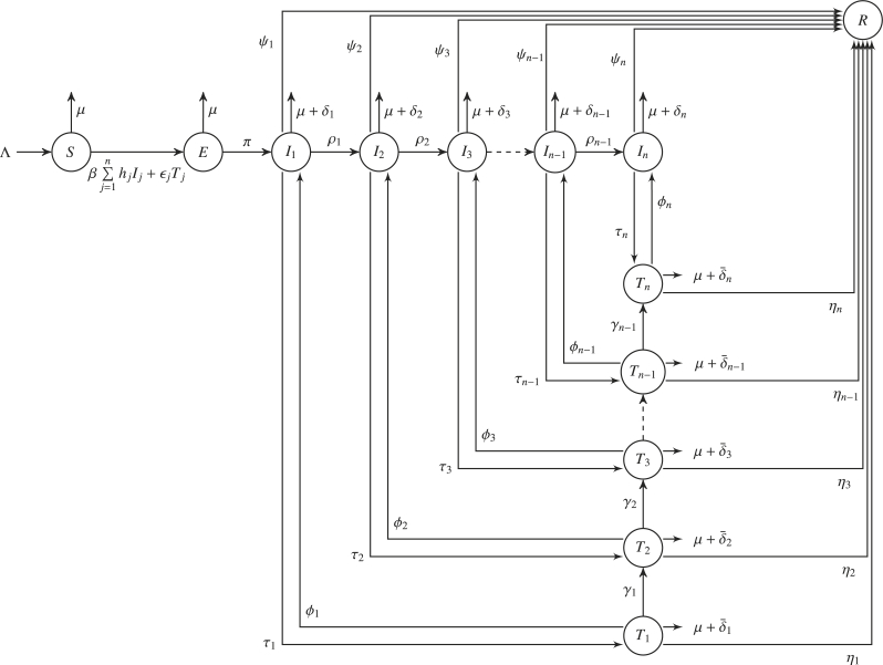
By assuming the human population is completely susceptible at the beginning of an epidemics and sub-dividing the total population, $N\left(t\right)$, into susceptible humans $S\left(t\right)$, exposed humans $E\left(t\right)$, infected untreated $I_j\left(t\right)$ humans in stage j of infection, infected humans under treatment and in stage j of infection $T_j\left(t\right)$, and the recovered population $R\left(t\right)$, at time t, we investigate the transmission and treatment of certain infectious diseases. We assume the total human population $N\left(t\right)$ satisfies $N\left(t\right)=S\left(t\right)+E\left(t\right)+\sum _{j=1}^n\left(I_j\left(t\right)+T_j\left(t\right)\right)+R\left(t\right)$ and humans are recruited into the susceptible population at a rate $\text{Λ}$. The general population is reduced by natural death at a rate μ. The population of susceptible humans is reduced by infection due to contact with infectious (untreated or treated) individual at a full rate $\beta \sum _{j=1}^n{h}_j{I}_j$. It is well known (Godoy et al., 2018) that influenza vaccination may not prevent infection but reduces the severity of the disease. The Center for Disease and Control 2 claimed that in randomized clinical trials, there was evidence that some influenza viruses developed resistance or reduced susceptibility to one or more influenza antiviral CDC recommended FDA-approved drugs like oseltamivir (Tamiflu), zanamivir (Relenza), peramivir (Rapivab), and baloxavir (Xofluza) ${\text{drugs}}^2$. Several authors (Feng et al., 2011; Gani et al., 2005; Kretzschmar, Schim van der Loeff, Birrell, Angelis, & Coutinho, 2013; Liu and Zhang, 2011; Otunuga, 2018; Qiu & Feng, 2010) have considered introducing parameter that accounts for the reduction in infectiousness due to treatments among individuals in their model. In our model, we let ${\mathrm{\epsilon }}_j$ be the reduced infectiousness due to treatment in stage j of infection and include the reduced rate $\beta \sum _{j=1}^n{\mathrm{\epsilon }}_j{T}_j$ due to treatment. Infected (but not yet infectious) individuals become untreated infectious individuals in stage 1 of infection at a rate π. Untreated infected individuals in stage k of infection migrate into stage $k+1$ of untreated infection at a rate ${\rho }_k$ and die of infection at a rate ${\delta }_k$. These individuals receive treatment (and migrate to stage k of treated infected compartment) at a rate ${\tau }_k$. Treated infected individuals in stage k of infection migrate to stage $k+1$ of treated infection at a rate ${\gamma }_k$ and die of infection at a rate ${\overline{\delta }}_k$. Individuals that stop receiving treatment migrate to stage k of untreated infected compartment at a rate ${\phi }_k$. Untreated and treated infected individuals in stage k of infection recover and migrate to the recovered compartment at a rate of ${\psi }_k$ and ${\eta }_k$, respectively. The schematics describing the transmission described above is given in Fig. 1.

Fig. 1.

Schematic diagram for the SEITR model. The circle compartments represent group of individuals.

The deterministic model governing S, E, $I_k$, $T_k$, R for $k=\mathrm{1,2},\dots ,n$, is described as follows:

$$\begin{array}{lll}dS\hfill & =\hfill & \left(\text{Λ}-\beta S\sum _{j=1}^n\left(h_j{I}_j+{\mathrm{\epsilon }}_j{T}_j\right)-\mu S\right)dt,S\left(t_0\right)=S_0,\hfill \\ dE\hfill & =\hfill & \left(\beta S\sum _{j=1}^n\left(h_j{I}_j+{\mathrm{\epsilon }}_j{T}_j\right)-\left(\mu +\pi \right)E\right)dt,E\left(t_0\right)=E_0,\hfill \\ d{I}_1\hfill & =\hfill & \left(\pi E-\left(\mu +{\delta }_1+{\rho }_1+{\tau }_1+{\psi }_1\right)I_1+{\phi }_1{T}_1\right)dt,I_1\left(t_0\right)=I_{01},\hfill \\ d{I}_k\hfill & =\hfill & \left({\rho }_{k-1}{I}_{k-1}-\left(\mu +{\delta }_k+{\rho }_k+{\tau }_k+{\psi }_k\right)I_k+{\phi }_k{T}_k\right)dt,I_k\left(t_0\right)=I_{0k},k=\mathrm{2,3},\dots ,n,\hfill \\ d{T}_1\hfill & =\hfill & \left({\tau }_1{I}_1-\left(\mu +{\overline{\delta }}_1+{\gamma }_1+{\phi }_1+{\eta }_1\right)T_1\right)dt,T_1\left(t_0\right)=T_{01},\hfill \\ d{T}_k\hfill & =\hfill & \left({\tau }_k{I}_k+{\gamma }_{k-1}{T}_{k-1}-\left(\mu +{\overline{\delta }}_k+{\gamma }_k+{\phi }_k+{\eta }_k\right)T_k\right)dt,T_k\left(t_0\right)=T_{0k},k=\mathrm{2,3},\dots ,n,\hfill \\ dR\hfill & =\hfill & \left(\sum _{j=1}^n\left({\psi }_j{I}_j+{\eta }_j{T}_j\right)-\mu R\right)dt,R\left(t_0\right)=R_0,\hfill \end{array}$$ (2.1)

where the parameters in the model are described in Table 2, with ${\gamma }_n={\rho }_n=0$. Since the limit $\underset{t\to \infty }{\text{lim}}\text{sup}N\left(t\right)\le \text{Λ}/\mu$, we consider the solution of the model (2.1) in the feasible region

$$\mathcal{T}:=\left\{{\left(S,E,I_1,\dots ,I_n,T_1,\dots ,T_n,R\right)}^T\in {\mathbb{R}}_{+}^{2n+3}:0\le S+E+\sum _{j=1}^n\left(I_j+T_j\right)+R=N\le \frac{\text{Λ}}{\mu }\right\},$$ (2.2)

where ${\mathbb{R}}_{+}$ denotes set of nonnegative real numbers. For the rest of this work, we define $\overline{\kappa }=\text{Λ}/\mu$. It can be shown that $\mathcal{T}$ is positively invariant with respect to (2.1). We set the sizes of S, E, $I_k$, $T_k$, R, for $k=\mathrm{1,2},\dots ,n$ as percentages by setting $\text{Λ}=\mu$.

Table 2.

Description of parameters for the epidemic model.

Parameter	Description
$\text{Λ}$	Recruitment rate into the population
β	Transmission rate of infection
$h_k$	Infectivity of untreated individuals in stage k of infection
${\epsilon }_k$	Reduced infectiousness due to treatment in stage k of infection
μ	Natural death rate
π	Infectious rate for exposed individuals
${\delta }_k$	Death rate associated with untreated infection in stage k of infection
${\overline{\delta }}_k$	Death rate associated with treated infection in stage k of infection
${\tau }_k$	Treatment rate of infected individuals in stage k of infection
${\phi }_k$	Rate of dropping out of treatment in stage k
${\rho }_k$	Transition rate from stage k to $k+1$ for untreated individuals
${\gamma }_k$	Transition rate from stage k to $k+1$ for treated individuals
${\psi }_k$	Recovery rate for untreated individuals in stage k of infection
${\eta }_k$	Recovery rate for treated individuals in stage k of infection

3. Existence of equilibrium points in the presence and absence of treatments

We discuss the existence and stability of the equilibrium points of (2.1) in the presence and absence of treatment. Under certain conditions (which are discussed in (3.14) and Section 5), system (2.1) has two unique equilibrium points namely, the disease-free (denoted $P_0$) and endemic (denoted $P_1$) equilibrium points described as

$$\begin{array}{c}{P}_0={\left(\begin{array}{ccccccccc}{\overline{S}}^0& {\overline{E}}^0& {\overline{I}}_1^0& \dots & {\overline{I}}_n^0& {\overline{T}}_1^0& \dots & {\overline{T}}_n^0& {\overline{R}}^0\end{array}\right)}^{\top },\\ P_1={\left(\begin{array}{ccccccccc}{\overline{S}}^{\ast }& {\overline{E}}^{\ast }& {\overline{I}}_1^{\ast }& \dots & {\overline{I}}_n^{\ast }& {\overline{T}}_1^{\ast }& \dots & {\overline{T}}_n^{\ast }& {\overline{R}}^{\ast }\end{array}\right)}^{\top }.\end{array}$$ (3.1)

The equilibrium points $P_0$ and $P_1$ are derived in 3.1, 3.2, respectively.

3.1. Disease-free equilibrium $P_0$

The disease-free equilibrium $P_0$ of (2.1) has entries

$${\overline{S}}^0=\overline{\kappa },{\overline{E}}^0=0,{\overline{I}}_j^0=0,{\overline{T}}_j^0=0,{\overline{R}}^0=0,j=\mathrm{1,2},\dots ,n.$$ (3.2)

In the following, we derive the measure of the power of an infectious disease to attack a completely susceptible population. It is the expected number of secondary cases produced, in a completely susceptible population, by a typical infective individual. This number, called the basic reproduction number and denoted by $R_{T,n}$, is calculated explicitly considering n stages of infection and treatment. The endemic equilibrium, $P_1$, is expressed in terms of $R_{T,n}$. We also discuss a case where no treatment is received in the population and denote the corresponding reproduction number by $R_{0,n}$. We show that in order for the number of infection to diminish to zero on the long run, appropriate parameters in the model must be controlled so that the number $R_{T,n}$ is at most one. That is, as long as the number of secondary infection produced by an infected individual is not more than one, the number of infections diminish to zero on the long run. Above the number $R_{T,n}=1$, disease endemic presist.

3.1.1. Elimination threshold quantity, $R_{T,n}$, in the presence of treatments

Define

$$\{\begin{array}{lll}{a}_k\hfill & =\hfill & \mu +{\delta }_k+{\rho }_k+{\tau }_k+{\psi }_k,\hfill \\ b_k\hfill & =\hfill & \mu +{\overline{\delta }}_k+{\gamma }_k+{\phi }_k+{\eta }_k,\hfill \\ c\hfill & =\hfill & \mu +\pi ,\hfill \\ \overline{\kappa }\hfill & =\hfill & \text{Λ}/\mu .\hfill \end{array}$$ (3.3)

In the presence of treatments, we write (2.1) in the form

$$d\mathbf{x}=\left(\mathcal{F}\left(\mathbf{x}\right)-\mathcal{V}\left(\mathbf{x}\right)\right)dt,$$ (3.4)

using the next-generation matrix (Driessche & Watmough, 2002), where.

$$\mathbf{x}=\left(\begin{array}{c}E\\ I_1\\ ⋮\\ I_n\\ T_1\\ ⋮\\ T_n\\ R\\ S\end{array}\right),\mathcal{F}={\left(\begin{array}{c}\beta S\sum _{j=1}^n\left(h_j{I}_j+{\mathrm{\epsilon }}_j{T}_j\right)\\ 0\\ ⋮\\ 0\\ 0\end{array}\right)}_{2n+3\times 1},\mathcal{V}=\left(\begin{array}{c}cE\\ a_1{I}_1-{\phi }_1{T}_1-\pi E\\ a_2{I}_2-{\rho }_1{I}_1-{\phi }_2{T}_2\\ ⋮\\ a_n{I}_n-{\rho }_{n-1}{I}_{n-1}-{\phi }_n{T}_n\\ b_1{T}_1-{\tau }_1{I}_1\\ b_2{T}_2-{\tau }_2{I}_2-{\gamma }_1{T}_1\\ ⋮\\ b_n{T}_n-{\tau }_n{I}_n-{\gamma }_{n-1}{T}_{n-1}\\ \mu R-\sum _{j=1}^n\left({\psi }_j{I}_j+{\eta }_j{T}_j\right)\\ \beta S\sum _{j=1}^n\left(h_j{I}_j+{\epsilon }_j{T}_j\right)+\mu S-\text{Λ}\end{array}\right).$$

The derivatives $D\mathcal{F}\left(P_0\right)=\left(\frac{\partial {\mathcal{F}}_i}{\partial {\mathbf{x}}_j}\right)=\left(\begin{array}{cc}{F}_n& 0_{2n+1\times 2}\\ 0_{2\times 2n+1}& 0_{2\times 2}\end{array}\right)$ and $D\mathcal{V}\left(P_0\right)=\left(\frac{\partial {\mathcal{V}}_i}{\partial {\mathbf{x}}_j}\right)=\left(\begin{array}{cc}{V}_n& 0_{2n+1\times 2}\\ J_3& J_4\end{array}\right)$ of $\mathcal{F}$ and $\mathcal{V}$, respectively, are evaluated at $P_0$ and partitioned so that $F_n=\beta \overline{\kappa }{\left(\begin{array}{ccccccccc}0& h_1& h_2& \dots & h_n& {\mathrm{\epsilon }}_1& {\mathrm{\epsilon }}_2& \dots & {\epsilon }_n\\ 0& 0& 0& \dots & 0& 0& 0& \dots & 0\\ 0& ⋮& ⋮& \ddots & ⋮& ⋮& ⋮& \ddots & ⋮\\ 0& 0& 0& \dots & 0& 0& 0& \dots & 0\end{array}\right)}_{2n+1\times 2n+1}$, $V_n=\left(\begin{array}{ccc}c& 0_{1\times n}& 0_{1\times n}\\ \mathit{\sigma }& M_I& -{\mathcal{I}}_{\phi }\\ 0_{n\times 1}& -{\mathcal{I}}_{\tau }& M_T\end{array}\right)$, $\mathit{\sigma }={{\left(\begin{array}{cccc}-\pi & 0& \dots & 0\end{array}\right)}^{\text{T}}}_{n\times 1}$, $J_3=\left(\begin{array}{ccccccccc}0& -{\psi }_1& -{\psi }_2& \dots & -{\psi }_n& -{\eta }_1& -{\eta }_2& \dots & -{\eta }_n\\ 0& \beta \overline{\kappa }{h}_1& \beta \overline{\kappa }{h}_2& \dots & \beta \overline{\kappa }{h}_n& \beta \overline{\kappa }{\mathrm{\epsilon }}_1& \beta \overline{\kappa }{\mathrm{\epsilon }}_2& \dots & \beta \overline{\kappa }{\mathrm{\epsilon }}_n\end{array}\right)$, $J_4=\left(\begin{array}{cc}\mu & 0\\ 0& \mu \end{array}\right)$, and

$$\begin{array}{llll}{M}_I\hfill & =\hfill & \left(\begin{array}{cccccc}{a}_1& 0& 0& 0& \dots & 0\\ -{\rho }_1& a_2& 0& 0& \dots & 0\\ 0& -{\rho }_2& a_3& 0& \dots & 0\\ ⋮& ⋮& ⋮& \ddots & \ddots & ⋮\\ ⋮& ⋮& ⋮& ⋮& \ddots & ⋮\\ 0& 0& \dots & 0& -{\rho }_{n-1}& a_n\end{array}\right),M_T=\left(\begin{array}{cccccc}{b}_1& 0& 0& 0& \dots & 0\\ -{\gamma }_1& b_2& 0& 0& \dots & 0\\ 0& -{\gamma }_2& b_3& 0& \dots & 0\\ ⋮& ⋮& ⋮& \ddots & \ddots & ⋮\\ ⋮& ⋮& ⋮& ⋮& \ddots & ⋮\\ 0& 0& \dots & 0& -{\gamma }_{n-1}& b_n\end{array}\right),\hfill & \hfill \\ {\mathcal{I}}_{\phi }\hfill & =\hfill & \text{diag}\left({\phi }_1,{\phi }_2,\cdots ,{\phi }_n\right),{\mathcal{I}}_{\tau }=\text{diag}\left({\tau }_1,{\tau }_2,\cdots ,{\tau }_n\right).\hfill & \hfill \end{array}$$ (3.5)

The spectral radius of the matrix $F_n{V}_n^{-1}$ is given by

$$R_{T,n}=\overline{\kappa }\beta \frac{\pi }{c}\sum _{k=1}^n\left[\frac{u_k{h}_k+{\mathrm{\epsilon }}_k{v}_k}{{\prod }_{j=1}^k\left(a_j{b}_j-{\tau }_j{\phi }_j\right)}\right],$$ (3.6)

where $u_k$ and $v_k$ satisfy

$$\{\begin{array}{l}{u}_k=b_k{\rho }_{k-1}{u}_{k-1}+{\phi }_k{\gamma }_{k-1}{v}_{k-1},\\ v_k={\tau }_k{\rho }_{k-1}{u}_{k-1}+a_k{\gamma }_{k-1}{v}_{k-1},\text{ for}k=\mathrm{1,2},\dots ,n,\end{array}$$ (3.7)

and ${\rho }_0={\gamma }_0=1$; $u_0=1$; $v_0=0$. We note here that $a_j{b}_j-{\tau }_j{\phi }_j={\overline{a}}_j{b}_j+{\tau }_j{\overline{b}}_j>0$ for $j=\mathrm{1,2},\dots ,n$.

Remark 3.1.1

The reproduction number (3.6) can be re-written in matrix form as

$$R_{T,n}=\overline{\kappa }\beta \frac{\pi }{c}\sum _{k=1}^n\left[\frac{\left(\begin{array}{cc}{h}_k& {\mathrm{\epsilon }}_k\end{array}\right)\left(\begin{array}{cc}{b}_k& {\phi }_k\\ {\tau }_k& a_k\end{array}\right)\left(\begin{array}{cc}{\rho }_{k-1}& 0\\ 0& {\gamma }_{k-1}\end{array}\right)\left(\begin{array}{c}{u}_{k-1}\\ v_{k-1}\end{array}\right)}{\prod _{j=1}^k\left|\left(\begin{array}{cc}{b}_j& {\phi }_j\\ {\tau }_j& a_j\end{array}\right)\right|}\right],$$ (3.8)

where $u_{k-1}$ and $v_{k-1}$ are defined in (3.7) and the matrices $\left(\begin{array}{cc}{b}_k& {\phi }_k\\ {\tau }_k& a_k\end{array}\right)$ and $\left(\begin{array}{cc}{\rho }_{k-1}& 0\\ 0& {\gamma }_{k-1}\end{array}\right)$ are coefficient matrices of the differential equation

$$\begin{array}{l}d\left(\begin{array}{c}{I}_k\\ T_k\end{array}\right)=\left(\begin{array}{cc}-a_k& {\varphi }_k\\ {\tau }_k& -b_k\end{array}\right)\left(\begin{array}{c}{I}_k\\ T_k\end{array}\right)+\left(\begin{array}{cc}{\rho }_{k-1}& 0\\ 0& {\gamma }_{k-1}\end{array}\right)\left(\begin{array}{c}{I}_{k-1}\\ T_{k-1}\end{array}\right)\\ =-\left|\left(\begin{array}{cc}{b}_k& {\varphi }_k\\ {\tau }_k& a_k\end{array}\right)\right|{\left(\begin{array}{cc}{b}_k& {\varphi }_k\\ {\tau }_k& a_k\end{array}\right)}^{-1}\left(\begin{array}{c}{I}_k\\ T_k\end{array}\right)+\left(\begin{array}{cc}{\gamma }_{k-1}& 0\\ 0& {\rho }_{k-1}\end{array}\right)\left(\begin{array}{c}{I}_{k-1}\\ T_{k-1}\end{array}\right),\end{array}$$

governing $I_k$ and $T_k$ in (2.1) for $k=\mathrm{2,3},\cdots ,n$.

Remark 3.1.2

Description of the derivation of $R_{T,n}$

For a model with one stage of infection, if $i,j=\mathrm{1,2,3}$ represent compartments $E,I_1$ and $T_1$, respectively, then the $\left(i,j\right)$ entry of the inverse $V_1^{-1}$ of the matrix $V_1$ defined in (3.5), and obtained as

$$V_1^{-1}=\left(\begin{array}{ccc}1/c& 0& 0\\ \frac{\pi }{c}\frac{b_1}{a_1{b}_1-{\tau }_1{\phi }_1}& \frac{b_1}{a_1{b}_1-{\tau }_1{\phi }_1}& \frac{{\phi }_1}{a_1{b}_1-{\tau }_1{\phi }_1}\\ \frac{\pi }{c}\frac{{\tau }_1}{a_1{b}_1-{\tau }_1{\phi }_1}& \frac{{\tau }_1}{a_1{b}_1-{\tau }_1{\phi }_1}& \frac{a_1}{a_1{b}_1-{\tau }_1{\phi }_1}\end{array}\right),$$ (3.9)

is the average time an individual introduced into compartment j spent in compartment i. It follows directly from (3.9) that the average time an individual introduced into the exposed compartment spent in the untreated infected compartment $I_1$ is $\frac{\pi }{c}\frac{b_1}{a_1{b}_1-{\tau }_1{\phi }_1}=\frac{1}{a_1}\frac{\pi }{c}\sum _{j=0}^{\infty }{\left(\frac{{\tau }_1}{a_1}\frac{{\phi }_1}{b_1}\right)}^j$, while the average time an individual introduced into the exposed compartment spent in the treated infected compartment $T_1$ is $\frac{\pi }{c}\frac{{\tau }_1}{a_1{b}_1-{\tau }_1{\phi }_1}=\frac{1}{b_1}\frac{\pi }{c}\sum _{j=1}^{\infty }{\left(\frac{{\tau }_1}{a_1}\right)}^j{\left(\frac{{\phi }_1}{b_1}\right)}^{j-1}$. An infected individual in the untreated and treated infected compartments $I_j$ and $T_j$ produces new infection in the exposed compartment E at a rate $\beta h_j$ and $\beta {\mathrm{\epsilon }}_j$, respectively. Thus, the number $R_{T,1}=\beta \overline{\kappa }{h}_1\frac{\pi }{c}\frac{b_1}{a_1{b}_1-{\tau }_1{\phi }_1}+\beta \overline{\kappa }{\mathrm{\epsilon }}_1\frac{\pi }{c}\frac{{\tau }_1}{a_1{b}_1-{\tau }_1{\phi }_1}$ is the expected number of secondary cases produced, in a completely susceptible population, by a typical infective individual in compartment 1. In general, the average time an individual introduced into the exposed compartment spent in the untreated infected compartment $I_k$ is $\frac{\pi }{c}\frac{u_k}{\prod _{j=1}^k\left(a_j{b}_j-{\tau }_j{\phi }_j\right)}$, while the average time an individual introduced into the exposed compartment spent in the treated infected compartment $T_k$ is $\frac{\pi }{c}\frac{v_k}{\prod _{j=1}^k\left(a_j{b}_j-{\tau }_j{\phi }_j\right)}$. Hence, $R_{T,n}=\beta \overline{\kappa }\frac{\pi }{c}\sum _{k=1}^n\left[\frac{u_k{h}_k+{\mathrm{\epsilon }}_k{v}_k}{\prod _{j=1}^k\left(a_j{b}_j-{\tau }_j{\phi }_j\right)}\right]$.

Remark 3.1.3

Reproduction number $R_{0,n}$ in the absence of treatment

Define

$$\{\begin{array}{ccc}{\overline{a}}_k& =& \mu +{\delta }_k+{\rho }_k+{\psi }_k,\\ {\overline{b}}_k& =& \mu +{\overline{\delta }}_k+{\gamma }_k+{\eta }_k.\end{array}$$ (3.10)

In the absence of treatment (that is, ${\tau }_k=0$ for $k=\mathrm{1,2},\dots ,n,$) we have $u_k=\prod _{j=1}^k\left(b_j{\rho }_{j-1}\right)$, $v_k=0$ for $k=\mathrm{1,2},\dots ,n,$ and the reproduction number $R_{T,n}$ simplifies to the treatment free reproduction number $R_{0,n}$ given by

$$R_{0,n}=\overline{\kappa }\beta \frac{\pi }{c}\sum _{k=1}^n\left[h_k\prod _{j=1}^k\left(\frac{{\rho }_{j-1}}{{\overline{a}}_j}\right)\right].$$ (3.11)

This is the reproduction number associated with the model without treatment

$$\begin{array}{lll}dS\hfill & =\hfill & \left(\text{Λ}-\beta S\sum _{j=1}^n\left(h_j{I}_j\right)-\mu S\right)dt,\hfill \\ dE\hfill & =\hfill & \left(\beta S\sum _{j=1}^n\left(h_j{I}_j\right)-\left(\pi +\mu \right)E\right)dt\hfill \\ d{I}_1\hfill & =\hfill & \left(\pi E-\left(\mu +{\delta }_1+{\rho }_1+{\psi }_1\right)I_1\right)dt,\hfill \\ d{I}_k\hfill & =\hfill & \left({\rho }_{k-1}{I}_{k-1}-\left(\mu +{\delta }_k+{\rho }_k+{\psi }_k\right)I_k\right)dt,k=\mathrm{2,3},\dots ,n\hfill \\ dR\hfill & =\hfill & \left(\sum _{j=1}^n{\psi }_j{I}_j-\mu R\right)dt.\hfill \end{array}$$ (3.12)

In a completely susceptible population receiving no treatment, we describe the quantity $R_{0,n}$ as the expected number of secondary infection produced by a typical untreated infected individual in a completely susceptible population.

The disease-free equilibrium point of (3.12) reduces to

$${\tilde{P}}_0={\left(\begin{array}{cccccc}{\tilde{S}}^0& {\tilde{E}}^0& {\tilde{I}}_1^0& \dots & {\tilde{I}}_n^0& {\tilde{R}}^0\end{array}\right)}^{\top },$$ (3.13)

3.2. Endemic equilibrium point, $P_1$, in the presence of treatment

The endemic equilibrium $P_1={\left(\begin{array}{ccccccccc}{\overline{S}}^{\text{*}}& {\overline{E}}^{\text{*}}& {\overline{I}}_1^{\text{*}}& \dots & {\overline{I}}_n^{\text{*}}& {\overline{T}}_1^{\text{*}}& \dots & {\overline{T}}_n^{\text{*}}& {\overline{R}}^{\text{*}}\end{array}\right)}^{\top }$ of system (2.1) described in (3.1) is obtained as

$$\{\begin{array}{llll}{\overline{S}}^{\text{*}}\hfill & =\hfill & \frac{\overline{\kappa }}{R_{T,n}},\hfill & \hfill \\ {\overline{E}}^{\text{*}}\hfill & =\hfill & \frac{\text{Λ}}{c}\left(1-\frac{1}{R_{T,n}}\right)\hfill & \hfill \\ {\overline{I}}_k^{\text{*}}\hfill & =\hfill & \frac{\pi }{c}\frac{\text{Λ}{u}_k}{\prod _{j=1}^k\left(a_j{b}_j-{\tau }_j{\phi }_j\right)}\left(1-\frac{1}{R_{T,n}}\right),\hfill & \hfill \\ {\overline{T}}_k^{\text{*}}\hfill & =\hfill & \frac{\pi }{c}\frac{\text{Λ}{v}_k}{\prod _{j=1}^k\left(a_j{b}_j-{\tau }_j{\phi }_j\right)}\left(1-\frac{1}{R_{T,n}}\right),k=\mathrm{1,2},\dots ,n,\hfill & \hfill \\ {\overline{R}}^{\text{*}}\hfill & =\hfill & \frac{\text{Λ}}{\mu }\frac{\pi }{c}\sum _{k=1}^n\left(\frac{u_k{\psi }_k+v_k{\eta }_k}{\prod _{j=1}^k\left(a_j{b}_j-\tau \phi \right)}\right)\left(1-\frac{1}{R_{T,n}}\right),\hfill & \hfill \end{array}$$ (3.14)

provided $R_{T,n}>1$, where $u_k$ and $v_k$ are defined in (3.7).

Remark 3.2.1

Endemic equilibrium in the absence of treatment.

In the absence of treatment, the endemic equilibrium $P_1$ reduces to

$${\tilde{P}}_1={\left(\begin{array}{cccccc}{\tilde{S}}^{\text{*}}& {\tilde{E}}^{\text{*}}& {\tilde{I}}_1^{\text{*}}& \dots & {\tilde{I}}_n^{\text{*}}& {\tilde{R}}^{\text{*}}\end{array}\right)}^{\top },$$ (3.15)

where ${\tilde{P}}_1$ is derived from (3.14) by setting ${\tau }_k=0$ and obtained as

$$\{\begin{array}{llll}{\tilde{S}}^{\text{*}}\hfill & =\hfill & \frac{\overline{\kappa }}{R_{0,n}},\hfill & \hfill \\ {\tilde{E}}^{\text{*}}\hfill & =\hfill & \frac{\text{Λ}}{c}\left(1-\frac{1}{R_{0,n}}\right),\hfill & \hfill \\ {\tilde{I}}_k^{\text{*}}\hfill & =\hfill & \frac{\pi }{c}\text{Λ}\left[\prod _{j=1}^k\left(\frac{{\rho }_{j-1}}{{\overline{a}}_j}\right)\right]\left(1-\frac{1}{R_{0,n}}\right),\hfill & \hfill \\ {\tilde{R}}^{\text{*}}\hfill & =\hfill & \frac{\text{Λ}}{\mu }\frac{\pi }{c}\sum _{k=1}^n\left({\psi }_k\prod _{j=1}^k\left(\frac{{\rho }_{j-1}}{{\overline{a}}_j}\right)\right)\left(1-\frac{1}{R_{0,n}}\right).\hfill & \hfill \end{array}$$ (3.16)

provided $R_{0,n}>1$.

4. Effect of treatment and dropping out treatment in the system

In this section, we study how receiving treatment and dropping out of treatment affect the system.

4.1. Effect of treatment of infection in the system

Consider the reproduction number $R_{T,j}$ corresponding to model (2.1) with j stage(s) of infection (derived by setting $n=j$ in (3.6)). Write $R_{T,j}\left({\tau }_i\right)\equiv R_{T,j}$ as a function of ${\tau }_i$ for $1\le i,j\le n$. We define the quantities $R_{T,j}({\tau }_i\to \infty )\equiv \underset{{\tau }_i\to \infty }{\text{lim}}{R}_{T,j}\left({\tau }_i\right)$ and $R_{T,j}({\tau }_i=0)\equiv R_{T,j}\left({\tau }_i\right){|}_{{\tau }_i=0}$ as the expected number of secondary infection produced by a typical infected individual (in a completely susceptible population with $j\le n$ stages of infection) as treatment capacity ${\tau }_i$ goes to infinity and as no treatment is administered in stage i of infection, respectively.

We can show, after rigorous calculations, that

$$\{\begin{array}{l}\{\begin{array}{lllll}{R}_{T,j}({\tau }_1\to \infty )\hfill & =\hfill & \overline{\kappa }\beta \frac{\pi }{c{\overline{b}}_1}\sum _{k=1}^j\frac{{\hat{u}}_k{h}_k+{\hat{v}}_k{\mathrm{\epsilon }}_k}{\prod _{\begin{array}{l}r=1\\ r\ne 1\end{array}}^k\left({\overline{a}}_r{b}_r+{\overline{b}}_r{\tau }_r\right)},\hfill & \hfill & \hfill \\ {\hat{u}}_1\hfill & =\hfill & 0,{\hat{v}}_1=1,\text{ and}{\hat{u}}_k,{\hat{v}}_k,k\ne 1\text{are defined in}\left(4.3\right)\hfill & \hfill & \hfill \end{array}\\ \{\begin{array}{lllll}{R}_{T,j}({\tau }_i\to \infty )\hfill & =\hfill & R_{T,i-1}+\overline{\kappa }\beta \frac{\pi }{c{\overline{b}}_i}\left(u_{i-1}{\rho }_{i-1}+v_{i-1}{\gamma }_{i-1}\right)\sum _{k=i}^j\frac{{\hat{u}}_k{h}_k+{\hat{v}}_k{\mathrm{\epsilon }}_k}{\prod _{\begin{array}{l}r=1\\ r\ne i\end{array}}^k\left({\overline{a}}_r{b}_r+{\overline{b}}_r{\tau }_r\right)},\text{ for}2\le i\le j\le n,\hfill & \hfill & \hfill \\ {\hat{u}}_i\hfill & =\hfill & 0,{\hat{v}}_i=1,\text{ and}{\hat{u}}_k,{\hat{v}}_k,k\ne i\text{are defined in}\left(4.3\right)\hfill & \hfill & \hfill \end{array}\end{array}$$ (4.1)

$$\{\begin{array}{l}\{\begin{array}{ccccc}{R}_{T,j}({\tau }_1=0)& =& \overline{\kappa }\beta \frac{\pi }{c{\overline{a}}_1}\sum _{k=1}^j\frac{{\check{u}}_k{h}_k+{\check{v}}_k{\mathrm{\epsilon }}_k}{\prod _{\begin{array}{l}r=1\\ r\ne 1\end{array}}^k\left({\overline{a}}_r{b}_r+{\overline{b}}_r{\tau }_r\right)},& & \\ {\check{u}}_1& =& 1,{\check{v}}_1=0,\text{ and}{\check{u}}_k,{\check{v}}_k,k\ne 1\text{are defined in}\left(4.3\right)& & \end{array}\\ \{\begin{array}{ccccc}{R}_{T,j}({\tau }_i=0)& =& R_{T,i-1}+\overline{\kappa }\beta \frac{\pi }{c{\overline{a}}_i{b}_i}\sum _{k=i}^j\frac{{\check{u}}_k{h}_k+{\check{v}}_k{\mathrm{\epsilon }}_k}{\prod _{\begin{array}{l}r=1\\ r\ne i\end{array}}^k\left({\overline{a}}_r{b}_r+{\overline{b}}_r{\tau }_r\right)},\text{ for}2\le i\le j\le n,& & \\ {\check{u}}_i& =& b_i{\rho }_{i-1}{\check{u}}_{i-1}+{\phi }_i{\gamma }_{i-1}{\check{v}}_{i-1},{\check{v}}_i={\overline{a}}_i{\gamma }_{i-1}{\check{v}}_{i-1},\text{ and}{\check{u}}_k,{\check{v}}_k,k\ne i\text{are defined in}\left(4.3\right),& & \end{array}\end{array}$$ (4.2)

where $u_i$, $v_i$ are defined in (3.7) for $i=\mathrm{1,2},\cdots ,n$, ${\check{u}}_0=1$, ${\check{v}}_0=0$, and

$$\{\begin{array}{l}\{\begin{array}{l}{\hat{u}}_k=b_k{\rho }_{k-1}{\hat{u}}_{k-1}+{\phi }_k{\gamma }_{k-1}{\hat{v}}_{k-1},\\ {\hat{v}}_k={\tau }_k{\rho }_{k-1}{\hat{u}}_{k-1}+a_k{\gamma }_{k-1}{\hat{v}}_{k-1},\text{ for}k=i+1,\cdots ,n,1\le i\le n\end{array}\\ \{\begin{array}{l}{\check{u}}_k=b_k{\rho }_{k-1}{\check{u}}_{k-1}+{\phi }_k{\gamma }_{k-1}{\check{v}}_{k-1},\\ {\check{v}}_k={\tau }_k{\rho }_{k-1}{\check{u}}_{k-1}+a_k{\gamma }_{k-1}{\check{v}}_{k-1},\text{ for}k\ne i.\end{array}\end{array}$$ (4.3)

Furthermore,

$$\{\begin{array}{l}\frac{d{R}_{T,j}}{d{\tau }_i}=\frac{{\overline{a}}_i{\overline{b}}_i{b}_i}{{\left({\overline{a}}_i{b}_i+{\overline{b}}_i{\tau }_i\right)}^2}(R_{T,j}({\tau }_i\to \infty )-R_{T,j}({\tau }_i=0)),\\ \frac{d^2{R}_{T,j}}{d{\tau }_i^2}=-\frac{2{\overline{a}}_i{\overline{b}}_i^2{b}_i}{{\left({\overline{a}}_i{b}_i+{\overline{b}}_i{\tau }_i\right)}^3}(R_{T,j}({\tau }_i\to \infty )-R_{T,j}({\tau }_i=0)),\text{for}1\le i,j\le n.\end{array}$$ (4.4)

It follows from (4.4) that the derivative $\frac{d{R}_{T,j}\left({\tau }_i\right)}{d{\tau }_i}<0$ and the graph of $R_{T,j}\left({\tau }_i\right)$ concaves up for all ${\tau }_i\ge 0$ if and only if $R_{T,j}({\tau }_i\to \infty )<R_{T,j}({\tau }_i=0),\text{for}1\le i\le j\le n$. Likewise, $\frac{d{R}_{T,j}}{d{\tau }_i}>0$ and the graph of $R_{T,j}\left({\tau }_i\right)$ concaves down for all ${\tau }_i\ge 0$ if and only if $R_{T,j}({\tau }_i\to \infty )>R_{T,j}({\tau }_i=0),\text{for}1\le i\le j\le n$. By definition, we expect $R_{T,j}({\tau }_i\to \infty )<R_{T,j}({\tau }_i=0),\text{for}1\le i,j\le n$. This shows that in a population with j stages of infection, the number of secondary infection, $R_{T,j}$, produced by an infected individual in a completely susceptible population decreases as the treatment rate ${\tau }_i$ increases.

4.1.1. Case where ${\tau }_i\equiv \tau$ for all $i=\mathrm{1,2},\cdots ,n$

Define

$$R_{\infty ,n}=\overline{\kappa }\beta \frac{\pi }{c}\sum _{k=1}^n\left[{\mathrm{\epsilon }}_k\prod _{j=1}^k\left(\frac{{\gamma }_{j-1}}{{\overline{b}}_j}\right)\right],$$ (4.5)

where ${\overline{b}}_j$ is defined in (3.10). For fixed ${\tau }_j=\tau$, $j=\mathrm{1,2},\cdots ,n$, we write $R_{T,n}\equiv R_{T,n}\left(\tau \right)$ (defined in (3.6)) as a function of τ. The number of secondary infection, $R_{T,n}\left(\tau \right)$, has the property:

$$R_{T,n}\to R_{\infty ,n}\text{ as}\tau \to \infty .$$

The function

$$f\left(\tau \right)=\frac{R_{T,n}\left(\tau \right)}{R_{0,n}},$$ (4.6)

is a rational function of τ referred to as the relative elimination threshold. The graph of the function has y-intercept $f\left(0\right)=1$ (following directly from Remark 3.1.1) and negative zeros. The vertical asymptotes are the negative vertical lines $\tau =-\frac{{\overline{a}}_j{b}_j}{{\overline{b}}_j}$, for $j=\mathrm{1,2},\cdots ,n$ . Define

$$\overline{f}=\frac{1}{R_{0,n}}\overline{\kappa }\beta \frac{\pi }{c}\sum _{k=1}^n\left[{\mathrm{\epsilon }}_k\prod _{j=1}^k\left(\frac{{\gamma }_{j-1}}{{\overline{b}}_j}\right)\right]=\frac{{\sum }_{k=1}^n\left[{\mathrm{\epsilon }}_k\prod _{j=1}^k\left(\frac{{\gamma }_{j-1}}{{\overline{b}}_j}\right)\right]}{{\sum }_{k=1}^n\left[h_k\prod _{j=1}^k\left(\frac{{\rho }_{j-1}}{{\overline{a}}_j}\right)\right]}.$$ (4.7)

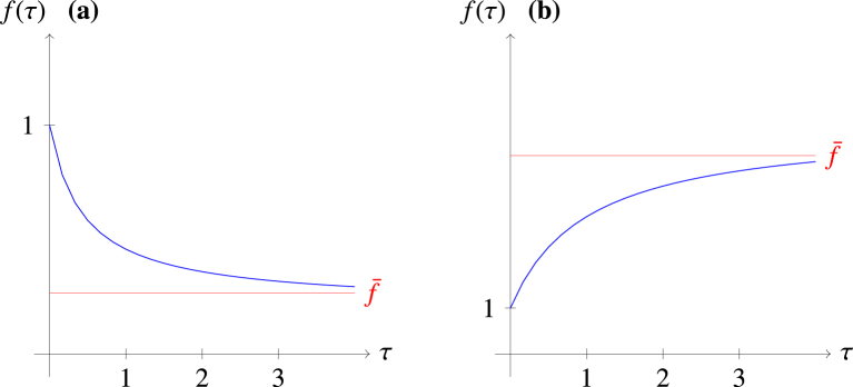
The function $f\left(\tau \right)\to \overline{f}$ as $\tau \to \infty$. The value $\overline{f}$ is the horizontal asymptote of $f\left(\tau \right)$. It measures the infection transmission potential when treatment capacity goes to infinity relative to the transmission potential when no treatment is administered. It follows from property of rational functions that $\overline{f}{R}_{0,n}<R_{T,n}\left(\tau \right)\le R_{0,n}$ $\left(\text{that is},R_{\infty ,n}<R_{T,n}\le R_{0,n}\right)$ if $\overline{f}<1$ and $R_{0,n}\le R_{T,n}\left(\tau \right)<\overline{f}{R}_{0,n}$ if $\overline{f}>1$. This is represented in Fig. 2 below.

Fig. 2.

Graphs of $f\left(\tau \right)$ against τ for the cases where $\overline{f}<1$ and $\overline{f}>1$.

Fig. 2 (a) and (b) show the trajectory of $f\left(\tau \right)$ for the cases where $\overline{f}<1$ and $\overline{f}>1$ , respectively.

Remark 4.1.1

The quantity $R_{\infty ,n}$ can be described as the expected number of secondary infection produced by a typical infected individual as the treatment capacity goes to infinity. From the description of $R_{0,n}$ in Remark 3.1.1, we expect $R_{\infty ,n}=\overline{\kappa }\beta \frac{\pi }{c}\sum _{k=1}^n\left[{\mathrm{\epsilon }}_k\prod _{j=1}^k\left(\frac{{\gamma }_{j-1}}{{\overline{b}}_j}\right)\right]<\overline{\kappa }\beta \frac{\pi }{c}\sum _{k=1}^n\left[h_k\prod _{j=1}^k\left(\frac{{\rho }_{j-1}}{{\overline{a}}_j}\right)\right]=R_{0,n}$, that is, we expect the expected number of secondary infection produced when the treatment capacity goes to infinity to be smaller than the expected number of secondary infection produced when no treatment is administered. This implies $\overline{f}<1$, so that $R_{T,n}<R_{0,n}$. This shows that as the treatment rate increases, the expected number of infection decreases. The highest expected number of infection produced by an infected individual in a completely susceptible population is $R_{0,n}$ (which is attained when $\tau =0$) while the lowest expected number of infection is $R_{\infty ,n}$ (attained as $\tau \to \infty$).

4.2. Effect of dropping out of treatment

Write $R_{T,j}\left({\phi }_i\right)\equiv R_{T,j}$ as a function of ${\phi }_i$ for $1\le i,j\le n$. Using similar definition in Subsection 4.1, we define the quantities $R_{T,j}({\phi }_i\to \infty )$ and $R_{T,j}({\phi }_i=0)$ as the expected number of secondary infection produced by a typical infected individual (in a completely susceptible population with $j\le n$ stages of infection) as drop out treatment rate ${\phi }_i$ goes to infinity and as no one drops out of treatment in stage i of infection, respectively.

We obtain, after rigorous calculations

$$\{\begin{array}{l}\{\begin{array}{l}{R}_{T,j}({\phi }_1\to \infty )=\overline{\kappa }\beta \frac{\pi }{c{\overline{a}}_1}\sum _{k=1}^j\frac{{\acute{u}}_k{h}_k+{\acute{v}}_k{\mathrm{\epsilon }}_k}{\prod _{\begin{array}{l}r=1\\ r\ne 1\end{array}}^k\left(a_r{\overline{b}}_r+{\overline{a}}_r{\phi }_r\right)},\\ {\acute{u}}_1=1,{\acute{v}}_1=0,\text{ and}{\acute{u}}_k,{\acute{v}}_k,k\ne 1\text{are defined in}\left(4.10\right),\end{array}\\ \{\begin{array}{l}{R}_{T,j}({\phi }_i\to \infty )=R_{T,i-1}+\overline{\kappa }\beta \frac{\pi }{c{\overline{a}}_i}\left(u_{i-1}{\rho }_{i-1}+v_{i-1}{\gamma }_{i-1}\right)\sum _{k=i}^j\frac{{\acute{u}}_k{h}_k+{\acute{v}}_k{\mathrm{\epsilon }}_k}{\prod _{\begin{array}{l}r=1\\ r\ne i\end{array}}^k\left(a_r{\overline{b}}_r+{\overline{a}}_r{\phi }_r\right)},\text{ for}2\le i\le j\le n,\\ {\acute{u}}_i=1,{\acute{v}}_i=0,\text{ and}{\acute{u}}_k,{\acute{v}}_k,k\ne i\text{are defined in}\left(4.10\right),\end{array}\end{array}$$ (4.8)

$$\{\begin{array}{l}\{\begin{array}{l}{R}_{T,j}({\phi }_1=0)=\overline{\kappa }\beta \frac{\pi }{c{a}_1{\overline{b}}_1}\sum _{k=1}^j\frac{{ü}_k{h}_k+{\ddot{v}}_k{\mathrm{\epsilon }}_k}{\prod _{\begin{array}{l}r=1\\ r\ne 1\end{array}}^k\left(a_r{\overline{b}}_r+{\overline{a}}_r{\phi }_r\right)},\\ {ü}_1={\overline{b}}_1,{\ddot{v}}_1={\tau }_1,\text{ and}{ü}_k,{\ddot{v}}_k,k\ne 1\text{are defined in}\left(4.10\right),\end{array}\\ \{\begin{array}{l}{R}_{T,j}({\phi }_i=0)=R_{T,i-1}+\overline{\kappa }\beta \frac{\pi }{c{a}_i{\overline{b}}_i}\sum _{k=i}^j\frac{{ü}_k{h}_k+{\ddot{v}}_k{\mathrm{\epsilon }}_k}{\prod _{\begin{array}{l}r=1\\ r\ne i\end{array}}^k\left(a_r{\overline{b}}_r+{\overline{a}}_r{\phi }_r\right)},\text{ for}2\le i\le j\le n,\\ {ü}_i={\overline{b}}_i{\rho }_{i-1}{ü}_{i-1},{\ddot{v}}_i={\tau }_i{\rho }_{i-1}{ü}_{i-1}+a_i{\gamma }_{i-1}{\ddot{v}}_{i-1},\text{ and}{ü}_k,{\ddot{v}}_k,k\ne i\text{are defined in}\left(4.10\right),\end{array}\end{array}$$ (4.9)

where $u_i$, $v_i$ are defined in (3.7) for $i=\mathrm{1,2},\cdots ,n$, ${ü}_0=1$, ${\ddot{v}}_0=0$, and

$$\{\begin{array}{l}\{\begin{array}{lll}{\acute{u}}_k\hfill & =\hfill & b_k{\rho }_{k-1}{\acute{u}}_{k-1}+{\phi }_k{\gamma }_{k-1}{\acute{v}}_{k-1},\hfill \\ {\acute{v}}_k\hfill & =\hfill & {\tau }_k{\rho }_{k-1}{\acute{u}}_{k-1}+a_k{\gamma }_{k-1}{\acute{v}}_{k-1},\text{ for}k=i+1,\cdots ,n,1\le i\le n\hfill \end{array}\\ \{\begin{array}{lll}{ü}_k\hfill & =\hfill & b_k{\rho }_{k-1}{ü}_{k-1}+{\phi }_k{\gamma }_{k-1}{\ddot{v}}_{k-1},\hfill \\ {\ddot{v}}_k\hfill & =\hfill & {\tau }_k{\rho }_{k-1}{ü}_{k-1}+a_k{\gamma }_{k-1}{\ddot{v}}_{k-1},\text{ for}k\ne i.\hfill \end{array}\end{array}$$ (4.10)

Furthermore,

$$\{\begin{array}{l}\frac{d{R}_{T,j}}{d{\phi }_i}=\frac{a_i{\overline{a}}_i{\overline{b}}_i}{{\left(a_i{\overline{b}}_i+{\overline{a}}_i{\phi }_i\right)}^2}(R_{T,j}({\phi }_i\to \infty )-R_{T,j}({\phi }_i=0)),\\ \frac{d^2{R}_{T,j}}{d{\phi }_i^2}=-\frac{2a_i{\overline{a}}_i^2{\overline{b}}_i}{{\left(a_i{\overline{b}}_i+{\overline{a}}_i{\phi }_i\right)}^3}(R_{T,j}({\phi }_i\to \infty )-R_{T,j}({\phi }_i=0)),\text{for}1\le i,j\le n.\end{array}$$ (4.11)

It follows from (4.11) that the derivative $\frac{d{R}_{T,j}\left({\phi }_i\right)}{d{\phi }_i}>0$ and the graph of $R_{T,j}\left({\phi }_i\right)$ concaves down for all ${\phi }_i\ge 0$ if and only if $R_{T,j}({\phi }_i\to \infty )>R_{T,j}({\phi }_i=0),\text{for}1\le i\le j\le n$. Likewise, $\frac{d{R}_{T,j}}{d{\phi }_i}<0$ and the graph of $R_{T,j}\left({\phi }_i\right)$ concaves up for all ${\phi }_i\ge 0$ if and only if $R_{T,j}({\phi }_i\to \infty )<R_{T,j}({\phi }_i=0),\text{for}1\le i\le j\le n$. By definition, we expect $R_{T,j}({\phi }_i\to \infty )>R_{T,j}({\phi }_i=0),\text{for}1\le i\le j\le n$. This shows that in a population with j stages of infection, the number of secondary infection, $R_{T,j}$, produced by an infected individual in a completely susceptible population increases as the treatment dropout rate ${\phi }_i$ increases.

4.2.1. Case where ${\phi }_i\equiv \phi$ for all $i=\mathrm{1,2},\cdots ,n$

Assume ${\phi }_j\equiv \phi$ for $j=\mathrm{1,2},\cdots ,n$, and write $R_{T,n}\equiv R_{T,n}\left(\phi \right)$. We see that

$$R_{T,n}\left(\phi \right)\to R_{0,n},\text{ as}\phi \to \infty ,$$

and

$$R_{T,n}(\phi =0)=\overline{\kappa }\beta \frac{\pi }{c}\stackrel{n}{\sum _{k=1}}\left[\stackrel{k}{\prod _{j=1}}\left(\frac{{\rho }_{j-1}}{a_j}\right)h_k+\frac{v_k}{\stackrel{k}{\prod _{j=1}}\left(a_j{\overline{b}}_j\right)}{\mathrm{\epsilon }}_k\right],$$

where $v_k$ is defined in (3.7) for $k=\mathrm{1,2},\cdots ,n$. The vertical asymptotes of the rational function $R_{T,n}\left(\phi \right)$ are the negative vertical lines $\phi =-a_j{\overline{b}}_j/{\overline{a}}_j$, for $j=\mathrm{1,2},\cdots ,n$. Since $R_{T,n}\left(\phi \right)$ is a rational function of φ whose numerator and denominator have the same degree, it follows that $R_{T,n}\left(\phi \right)$ is an increasing function of φ if and only if $R_{T,n}(\phi =0)\le R_{T,n}(\phi \to \infty )=R_{0,n}$, for $\phi \ge 0$. By definition, we expect $R_{T,n}(\phi =0)\le R_{T,n}(\phi \to \infty )$. This shows that as the rate of dropping out of treatment increases, the expected number of secondary infection produced by an infected individual increases to $R_{0,n}$.

4.2.2. Numerical results verifying the effects of treatment and dropping out of treatment on the number of infections

Here, we use relevant parameters to the transmission dynamics of influenza disease in the United States for the numerical simulations of the reproduction number as a function of the treatment and dropout rates. We set the life expectancy of the United States population to 80 years3 and the total population to be $\mathrm{329,256,465}$ as of July 2018.4 Using the parameters collected from the Center for Disease Control and Prevention (CDC), the time from when a person is exposed and infected with flu to when symptoms begin is about 2 days, but can range from about 1 to 4 days5 and uncomplicated influenza signs and symptoms typically resolve after 3–7 days for the majority of people.6 Antiviral drugs, when used for treatment, can reduce symptoms and shorten sick time by 1 or 2 ${\text{days}}^6$.

CDC7 estimates that, from October 1, 2018, through May 4, 2019, there have been $37.4-42.9$ million flu illness, $17.3-20.1$ million flu medical visits, $531-647$ thousand flu hospitalizations and $36.4-61.2$ thousand flu death. We define ${\mathrm{\epsilon }}_j$ as a reduction factor in infectiousness (in stage j of infection) due to flu treatment and it reduces the infectious period to ${\frac{1}{\eta }}_j<{\frac{1}{\psi }}_j$. For more information about the parameter ${\mathrm{\epsilon }}_j$, we refer readers to the work of Lipsitch et al. (Liu & Zhang, 2011), Feng et al. (Feng et al., 2011), Kretzschmar et al. (Kretzschmar et al., 2013) and ${\text{CDC}}^2$. In their work, Lipsitch (Liu and Zhang, 2011) introduced a parameter which is the reduction in hazard of infection for an individual on prophylaxis. They claimed with probability $e_p$, transmission is blocked and of those blocked infections, a proportion $a_p$ are only partially blocked. Using two infectious stages, we set $\frac{1}{{\rho }_1}=4$, $\frac{1}{{\rho }_2}=3$, $\frac{1}{{\gamma }_1}=4$, $\frac{1}{{\gamma }_2}=2$, $\beta =0.8$, $h_1=0.5$, $h_2=0.106$, ${\mathrm{\epsilon }}_1=0.2$, ${\mathrm{\epsilon }}_2=0.05$, ${\tau }_1=0.08$, ${\tau }_2=0.12$, ${\phi }_1=1/3$, ${\phi }_2=1/4$, ${\psi }_1=1/5$, ${\psi }_2=1/10$, ${\eta }_1=1/4$, ${\eta }_2=1/8$, ${\delta }_1=1.43\times {10}^{-4}$, ${\delta }_2=1.1\times {10}^{-4}$, ${\overline{\delta }}_1=0.925\times {10}^{-4}$, ${\overline{\delta }}_2=0.8\times {10}^{-4}$. The value $\frac{20.1}{329.27}$ for the number $\sum _{j=1}^n{T}_j\left(0\right)$ of individuals under treatment is close to the number reported by Biggerstaff et al. (Biggerstaff, Jhung, Kamimoto, Balluz, & Finelli, 2012). According to the paper published by Tokars at al. (Tokars, Olsen, & Reed, 2018), between $3\text{\%}$ and $11.3\text{\%}$ of the U.S. population gets infected and develops flu symptoms each year. The value $\frac{37.4}{329.27}$ is approximately in this reported range. See Table 1, Table 2, Table 3 for parameter values and descriptions.

Table 1.

Description of variables for the epidemic model.

Variable	Description
S	Population of susceptible individuals
E	Population of exposed individuals
$I_k$	Population of untreated infected individuals in stage k of infection
$T_k$	Population of treated infected individuals in stage k of infection
R	Population of individuals who recovered from disease

Table 3.

Parameter values for the epidemic model: Case study Influenza.

Parameter	Description	Default Value	References
$\text{Λ}$	Recruitment rate into the population	$\frac{1}{80\times 365}{\text{day}}^{-1}$	${\text{CIA}}^3$
β	Transmission rate of infection	$\sum _{j=1}^n\beta h_j=0.5$	Feng et al. (2011)
$h_k$	Infectivity of untreated individuals in stage k of infection	0.5	(Feng et al., 2011; Roosa & Chowell, 2019)
${\epsilon }_k$	Reduced infectiousness due to treatment in stage k of infection	0.2	Feng et al. (2011)
π	Infectious rate for exposed individuals	$\frac{1}{\pi }=2$ (days)	${\text{CDC}}^5$
μ	Natural death rate	$\text{Λ}$	${\text{CIA}}^3$
${\delta }_k$	Death rate associated with untreated infection	$1.43\times {10}^{-4}$	Murphy, Xu, Kochanek, and Arias (2018)
${\overline{\delta }}_k$	Death rate associated with treated infection		Assumed
${\tau }_k$	Treatment rate of individuals in stage k of infection	$\sum _{j=1}^n{\tau }_j\in [0.05,0.2]$ (${\text{day}}^{-1}$)	${\text{CDC}}^6$
${\phi }_k$	Rate of dropping out of treatment in stage k	$\sum _{j=1}^n\frac{1}{{\phi }_j}=7$ (days)	Assumed
${\rho }_k$	Average duration of untreated infection	$\sum _{j=1}^n\frac{1}{{\rho }_j}\in \left[\mathrm{3,7}\right]$ (days)	${\text{CDC}}^6$
${\gamma }_k$	Average duration of treated infection	$\sum _{j=1}^n\frac{1}{{\gamma }_j}\in \left[\mathrm{1,6}\right]$ (days)	${\text{CDC}}^6$
${\psi }_k$	Recovery rate for untreated individuals in stage k of infection	$\sum _{j=1}^n\frac{1}{{\psi }_j}\in \left[\mathrm{3,15}\right]$ (days)	(Feng et al., 2011; Roosa & Chowell, 2019)$\&$ Assumed
${\eta }_k$	Recovery rate for treated individuals in stage k of infection	$\sum _{j=1}^n\frac{1}{\eta j}\in \left[\mathrm{2,14}\right]$ (days)	(Feng et al., 2011; Roosa & Chowell, 2019)$\&$ Assumed
$S\left(0\right)$	Initial susceptible Population		Assumed
$E\left(0\right)$	Initial Exposed Population		Assumed
$\sum _{j=1}^n{I}_j\left(0\right)$	Initial Untreated Infected Population	$\frac{37.4}{329.27}$	${\text{CIA}}^3$, ${\text{CDC}}^7$
$\sum _{j=1}^n{T}_j\left(0\right)$	Initial Treated Infected Population	$\frac{20.1}{329.27}$	${\text{CIA}}^3$, ${\text{CDC}}^7$
$R\left(0\right)$	Initial Recovered Population		Assumed

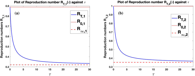
Fig. 3 (a) shows the graph of $R_{T,1}\equiv R_{T,1}\left(\tau \right)$ against $\tau \equiv {\tau }_1$. Fig. 3 (b) shows the graph of $R_{T,2}\equiv R_{T,2}\left(\tau \right)$ against $\tau \equiv {\tau }_1={\tau }_2$. The graphs show that with no treatment, the reproduction number is $R_{0,n}$, and as more treatment is introduced into the population the number of secondary infection $R_{T,n}$ reduces until it approaches $R_{\infty ,n}$, which is the least number of secondary infection that can be produced by an infected individuals when introduced into susceptible population. This is explained in Subsection 4.1.

Fig. 3.

Effect of treatment on the reproduction number $R_{T,n}$ for $n=1$ and $n=2$.

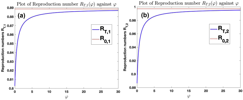
Fig. 4 (a) shows the graph of $R_{T,1}\equiv R_{T,1}\left(\phi \right)$ against $\phi \equiv {\phi }_1$. Fig. 4 (b) shows the graph of $R_{T,2}\equiv R_{T,2}\left(\phi \right)$ against $\phi \equiv {\phi }_1={\phi }_2$. The graphs show that the number of secondary infection $R_{T,n}$ increases to $R_{0,n}$ as individuals drop out of treatment. This is explained in Subsection 4.2.

Fig. 4.

Effect of dropping out of treatment on the reproduction number $R_{T,n}$ for cases $n=1$ and $n=2$.

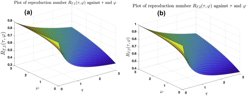
Fig. 5 (a) shows the graph of $R_{T,1}\equiv R_{T,1}\left(\tau ,\phi \right)$ against $\tau \equiv {\tau }_1$ and $\phi \equiv {\phi }_1$. Fig. 5 (b) shows the graph of $R_{T,2}\left(\tau ,\phi \right)$ against $\tau \equiv {\tau }_1={\tau }_2$ and $\phi \equiv {\phi }_1={\phi }_2$.

Fig. 5.

Effect of treatment and dropping out of treatment on the reproduction number for the cases $n=1$ and $n=2$, and $R_{T,n}<1$.

5. Existence and stability of equilibrium points

In this section, we discuss the endpoint behavior of the solution of (2.1). We give conditions under which the solution converges on the long run to the disease-free or endemic equilibrium.

5.1. Existence and stability of disease-free equilibrium $P_0$ in the presence of treatment

The following theorems show the condition for the local and global stability of the disease-free equilibrium, $P_0$. We study condition(s) under which disease elimination exists on the long run. The idea presented here is similar to the work in Otunuga (Otunuga, 2018). To analyze the local asymptotic stability of $P_0$, we linearize (2.1) about $P_0$ and show that the real part of all eigenvalues of the coefficient matrix of the linear associated system is negative.

Define $\mathrm{\Psi }={\left(\begin{array}{ccccc}S-\overline{\kappa }& E& I_1\dots I_n& T_1\dots T_n& R\end{array}\right)}^{\top }$. The linearization of (2.1) along the disease-free equilibrium $P_0$ is obtained as

$$d\mathrm{\Psi }=\mathbf{A}\mathrm{\Psi }dt,\mathrm{\Psi }\left(t_0\right)={\mathrm{\Psi }}_0,$$ (5.1)

where $\mathbf{A}=\left(\begin{array}{cccc}{A}_{\mathrm{1,1}}& A_{\mathrm{1,2}}& A_{\mathrm{1,3}}& A_{\mathrm{1,4}}\\ A_{\mathrm{2,1}}& A_{\mathrm{2,2}}& A_{\mathrm{2,3}}& A_{\mathrm{2,4}}\\ A_{\mathrm{3,1}}& A_{\mathrm{3,2}}& A_{\mathrm{3,3}}& A_{\mathrm{3,4}}\\ A_{\mathrm{4,1}}& A_{\mathrm{4,2}}& A_{\mathrm{4,3}}& A_{\mathrm{4,4}}\end{array}\right)$ with $A_{\mathrm{1,1}}=\left(\begin{array}{cc}-\mu & 0\\ 0& -c\end{array}\right)$, $A_{\mathrm{1,2}}=\beta \overline{\kappa }\left(\begin{array}{cccc}-h_1& -h_2& \dots & -h_n\\ h_1& h_2& \dots & h_n\end{array}\right)$, $A_{\mathrm{1,3}}=\beta \overline{\kappa }\left(\begin{array}{cccc}-{\mathrm{\epsilon }}_1& -{\mathrm{\epsilon }}_2& \dots & -{\mathrm{\epsilon }}_n\\ {\mathrm{\epsilon }}_1& {\mathrm{\epsilon }}_2& \dots & {\mathrm{\epsilon }}_n\end{array}\right)$, $A_{\mathrm{1,4}}=\left(\begin{array}{c}0\\ 0\end{array}\right)$, $A_{\mathrm{2,1}}=\left(\begin{array}{cc}{0}_{1\times 1}& \pi \\ 0_{n-1\times 1}& 0_{n-1\times 1}\end{array}\right)$, $A_{\mathrm{2,2}}=-M_I$, $A_{\mathrm{2,3}}={\mathcal{I}}_{\phi }$, $A_{\mathrm{2,4}}=A_{\mathrm{3,4}}=\left(\begin{array}{c}{0}_{n\times 1}\end{array}\right)$, $A_{\mathrm{3,1}}=\left(\begin{array}{c}{0}_{n\times 2}\end{array}\right)$, $A_{\mathrm{3,2}}={\mathcal{I}}_{\tau }$, $A_{\mathrm{3,3}}=-M_T$, $A_{\mathrm{4,1}}=\left(\begin{array}{c}{0}_{1\times 2}\end{array}\right)$, $A_{\mathrm{4,2}}=\left(\begin{array}{cc}{\psi }_1& {\psi }_2\cdots {\psi }_n\end{array}\right)$, $A_{\mathrm{4,3}}=\left(\begin{array}{cc}{\eta }_1& {\eta }_2\cdots {\eta }_n\end{array}\right)$, $A_{\mathrm{4,4}}=-d$, and $M_I,M_T,{\mathcal{I}}_{\phi },{\mathcal{I}}_{\tau }$ are defined in (3.5). We can express the characteristic polynomial of A in the form

$$det\left(\mathbf{A}-r{\mathcal{I}}_{2n+3\times 2n+3}\right)=-\left(r+\mu \right)det\left(\overline{\mathbf{A}}-r{\mathcal{I}}_{2n+2\times 2n+2}\right),$$ (5.2)

where $\overline{\mathbf{A}}$ is the square matrix formed by deleting the first row and column of A in (5.1) and r is the eigenvalue of A.

Theorem 5.1

The real part of all eigenvalues of A is negative if $R_{T,n}<1$. One of the eigenvalues of A is zero if $R_{T,n}=1$ and at least one of the eigenvalues is positive real if $R_{T,n}>1$.

Proof. It suffices to show that the maximum real part of all eigenvalues of $\overline{\mathbf{A}}$, denoted, $s\left(\overline{\mathbf{A}}\right)$, is less than zero if $R_{T,n}<1$. To do this, we use relations $D_{12}$ and $J_{29}$ in (Plemmons, 1977) to show that the real part of each eigenvalues of the matrix $\mathcal{B}=-\mathbf{A}$ is positive. The matrix can be written in the form

$$\mathcal{B}=\mathcal{L}\mathcal{U},$$ (5.3)

where $\mathcal{L}$ and $\mathcal{U}$ are lower and upper diagonal matrices, respectively, with positive diagonals. The matrices $\mathcal{L}=\left({\mathcal{L}}_{i,j}\right)$ and $\mathcal{U}=\left({\mathcal{U}}_{i,j}\right)$ are computed rigorously as follows:

$${\mathcal{L}}_{i,j}=\frac{1}{{\mathcal{D}}_j}\left|\begin{array}{cccc}{\mathcal{B}}_{\mathrm{1,1}}& {\mathcal{B}}_{\mathrm{1,2}}& \dots & {\mathcal{B}}_{1,j}\\ {\mathcal{B}}_{\mathrm{2,1}}& {\mathcal{B}}_{\mathrm{2,2}}& \dots & {\mathcal{B}}_{2,j}\\ ⋮& ⋮& \dots & ⋮\\ {\mathcal{B}}_{j-\mathrm{1,1}}& {\mathcal{B}}_{j-\mathrm{1,2}}& \dots & {\mathcal{B}}_{j-1,j}\\ {\mathcal{B}}_{i,1}& {\mathcal{B}}_{i,2}& \dots & {\mathcal{B}}_{i,j}\end{array}\right|,\text{ for}i\ge j\ne 1,{\mathcal{L}}_{i,1}=\frac{\left|{\mathcal{B}}_{i,1}\right|}{{\mathcal{D}}_1}\text{ for}i=\mathrm{1,2},\dots ,2n+2,\text{ and}0\text{ elsewhere},$$

$${\mathcal{U}}_{i,j}=\frac{1}{{\mathcal{D}}_{i-1}}\left|\begin{array}{cccc}{\mathcal{B}}_{\mathrm{1,1}}& \dots & {\mathcal{B}}_{1,i-1}& {\mathcal{B}}_{1,j}\\ {\mathcal{B}}_{\mathrm{2,1}}& \dots & {\mathcal{B}}_{2,i-1}& {\mathcal{B}}_{2,j}\\ ⋮& ⋮& ⋮& ⋮\\ {\mathcal{B}}_{i,1}& \dots & {\mathcal{B}}_{i,i-1}& {\mathcal{B}}_{i,j}\end{array}\right|,\text{ for}1\ne i\le j,{\mathcal{U}}_{1,j}={\mathcal{B}}_{1,j},\text{for}j=\mathrm{1,2},\dots ,2n+2,\text{and}0\text{ elsewhere},$$

where ${\mathcal{D}}_0:=1$, and ${\mathcal{D}}_j=\left|\begin{array}{cccc}{\mathcal{B}}_{\mathrm{1,1}}& {\mathcal{B}}_{\mathrm{1,2}}& \dots & {\mathcal{B}}_{1,j}\\ {\mathcal{B}}_{\mathrm{2,1}}& {\mathcal{B}}_{\mathrm{2,2}}& \dots & {\mathcal{B}}_{2,j}\\ ⋮& ⋮& \dots & ⋮\\ {\mathcal{B}}_{j,1}& {\mathcal{B}}_{j,2}& \dots & {\mathcal{B}}_{j,j}\end{array}\right|$ for $j=\mathrm{1,2},\dots ,2n+2$, and can be simplified as

$$\begin{array}{lllll}{a}_0\hfill & =\hfill & 1,{\overline{\overline{R}}}_{\mathrm{0,0}}=0,\hfill & \hfill & \hfill \\ {\overline{\overline{R}}}_{0,j}\hfill & =\hfill & \overline{\kappa }\beta \frac{\pi }{c}\sum _{k=1}^j\left[h_k\prod _{r=1}^k\left(\frac{{\rho }_{r-1}}{a_r}\right)\right],j=\mathrm{1,2},\cdots ,n+1\hfill & \hfill & \hfill \\ {\overline{\overline{R}}}_{T,j}\hfill & =\hfill & R_{T,j}+\overline{\kappa }\beta \frac{\pi }{c}\frac{u_j}{\prod _{k=1}^j\left(a_k{b}_k-{\tau }_k{\phi }_k\right)}\sum _{k=j+1}^n\left[h_k\prod _{r=j+1}^k\left(\frac{{\rho }_{r-1}}{a_r}\right)\right],j=\mathrm{1,2},\cdots ,n-1\hfill & \hfill & \hfill \\ {\mathcal{D}}_j\hfill & =\hfill & c\left[\prod _{k=0}^{j-1}{a}_k\right]\left(1-{\overline{\overline{R}}}_{0,j-1}\right),\text{ for}j=\mathrm{1,2},\cdots ,n+1,\hfill & \hfill & \hfill \\ {\mathcal{D}}_{n+1+j}\hfill & =\hfill & c\left[\prod _{k=1}^j\left(a_k{b}_k-{\tau }_k{\phi }_k\right)\right]\left(\prod _{k=j+1}^n{a}_k\right)\left(1-{\overline{\overline{R}}}_{T,j}\right),\text{ for}j=\mathrm{1,2},\cdots ,n-1,\hfill & \hfill & \hfill \\ {\mathcal{D}}_{2n+1}\hfill & =\hfill & c\left[\prod _{k=1}^n\left(a_k{b}_k-{\tau }_k{\phi }_k\right)\right]\left(1-R_{T,n}\right),\hfill & \hfill & \hfill \\ {\mathcal{D}}_{2n+2}\hfill & =\hfill & c\mu \left[\prod _{k=1}^n\left(a_k{b}_k-{\tau }_k{\phi }_k\right)\right]\left(1-R_{T,n}\right),\hfill & \hfill & \hfill \end{array}$$ (5.4)

where $|.|$ is the determinant operator, $\left\{a_k,b_k\right\}$ and { $R_{T,n},u_k$} are defined in (3.3) and (3.6), respectively. Since $u_k>u_j\prod _{r=j+1}^k\left(b_r{\rho }_{r-1}\right)$ and $\prod _{r=j+1}^k\left(a_r{b}_r\right)>\prod _{r=j+1}^k\left(a_r{b}_r-{\tau }_r{\phi }_r\right)$ for $k=j+1,\cdots ,n$, it follows that $\overline{\kappa }\beta \frac{\pi }{c}\frac{u_j}{\prod _{k=1}^j\left(a_k{b}_k-{\tau }_k{\phi }_k\right)}\sum _{k=j+1}^n\left[h_k\prod _{r=j+1}^k\left(\frac{{\rho }_{r-1}}{a_r}\right)\right]=\overline{\kappa }\beta \frac{\pi }{c}\sum _{k=j+1}^n\left[\frac{h_k{u}_j\prod _{r=j+1}^k\left(b_r{\rho }_{r-1}\right)}{\prod _{r=1}^j\left(a_r{b}_r-{\tau }_r{\phi }_r\right)\prod _{r=j+1}^k\left(a_r{b}_r\right)}\right]<\overline{\kappa }\beta \frac{\pi }{c}\sum _{k=j+1}^n\left[\frac{h_k{u}_k}{\prod _{r=1}^k\left(a_r{b}_r-{\tau }_r{\phi }_r\right)}\right]$ and so ${\overline{\overline{R}}}_{T,j}<R_{T,n}$ for $j=\mathrm{1,2},\cdots ,n-1$. Therefore, if $R_{T,n}<1$, it follows from (5.4) that ${\overline{\overline{R}}}_{0,j-1}<R_{T,n}$ for $j=\mathrm{1,2},\cdots ,n+1$, ${\mathcal{D}}_j>0$ and the diagonal entries ${\mathcal{U}}_{j,j}=\frac{{\mathcal{D}}_j}{{\mathcal{D}}_{j-1}}>0$ for $j=\mathrm{1,2},\cdots ,2n+2$. Since $\mathcal{B}\in Z^{2n+2}$ is a Z-matrix $\left(\text{that is},b_{i,j}\le 0\text{if}i\ne j,1\le i,j\le 2n+2,\text{where}\mathcal{B}=\left(b_{i,j}\right)\right)$ and the diagonal entries ${\mathcal{L}}_{j,j}=\frac{{\mathcal{D}}_j}{{\mathcal{D}}_j}=1$ for $j=\mathrm{1,2},\dots ,2n+2$, it follows from relations $D_{12}$ and $J_{29}$ in (Plemmons, 1977) that the real part of each eigenvalues of matrix $\mathcal{B}$ is positive, which is in turn equivalent to $s\left(\overline{\mathbf{A}}\right)<0$. The determinant of the matrix $\overline{\mathbf{A}}$ is $D_{2n+2}$, which is the product of all $2n+2$-eigenvalues of $\overline{\mathbf{A}}$. If $R_{T,n}=1$, then $D_{2n+2}=0$, which means at least one of the eigenvalues of $\overline{\mathbf{A}}$ is zero. If $R_{T,n}>1$, then $D_{2n+2}<0$, which means at least one of the eigenvalues of $\overline{\mathbf{A}}$ is positive. $■$

Theorem 5.2

The disease-free equilibrium $P_0$ of (2.1) is locally asymptotically stable if $R_{T,n}<1$ and unstable if $R_{T,n}>1$.

Proof. The proof follows from (5.2) and Theorem 5.1. $■$

The above theorem shows that if $R_{T,n}<1$, the system $\left(S,E,I_1,\cdots ,I_n,T_1,\cdots ,T_n,R\right)$ approaches the equilibrium point $P_0$ whenever it starts somewhere near it in $\mathcal{T}$. The local stability of the disease-free equilibrium ${\tilde{P}}_0$ of system (3.12) without treatment follows immediately from Theorem 5.2 by setting ${\tau }_k=0$ for all $k=\mathrm{1,2},\cdots ,n$. We state the theorem below without proof.

Corollary 5.3

The disease-free equilibrium ${\tilde{P}}_0$ of (3.12) is locally asymptotically stable if $R_{0,n}<1$ and unstable if $R_{0,n}>1$.

The following theorem gives the threshold under which disease elimination (considered independent of the initial conditions in $\mathcal{T}$) exists.

Theorem 5.4

The disease-free equilibrium $P_0$ of (2.1) is globally stable in the feasible region $\mathcal{T}$ if $R_{T,n}\le 1$.

Proof. Define the Lyapunov function $L:{\mathbb{R}}_{2n+2}^{+}\to {\mathbb{R}}^{+}$ by

$$L\left(S,E,I_1,I_2,\dots ,I_n,T_1,\dots ,T_n\right)=\left(S-{\overline{S}}^0-{\overline{S}}^0\ln \frac{S}{{\overline{S}}^0}\right)+\varpi E+\sum _{k=1}^n{\hat{\varphi }}_k{I}_k+\sum _{k=1}^n{\hat{\theta }}_k{T}_k,$$ (5.5)

where ${\mathbb{R}}^{+}$ is the set of positive real numbers, ϖ, ${\hat{\varphi }}_k$ and ${\hat{\theta }}_k$ satisfy

$$\begin{array}{llll}\varpi \hfill & =\hfill & 1,\hfill & \hfill \\ \left(\begin{array}{c}{\hat{\varphi }}_n\\ {\hat{\theta }}_n\end{array}\right)\hfill & =\hfill & \frac{\beta {\overline{S}}^0}{a_n{b}_n-{\tau }_n{\phi }_n}\left(\begin{array}{c}{h}_n{b}_n+{\tau }_n{\mathrm{\epsilon }}_n\\ h_n{\phi }_n+a_n{\mathrm{\epsilon }}_n\end{array}\right),\hfill & \hfill \\ \left(\begin{array}{c}{\hat{\varphi }}_{n-k}\\ {\hat{\theta }}_{n-k}\end{array}\right)\hfill & =\hfill & \frac{1}{a_{n-k}{b}_{n-k}-{\tau }_{n-k}{\phi }_{n-k}}\left[\left(\begin{array}{cc}{b}_{n-k}{\rho }_{n-k}& {\gamma }_{n-k}{\tau }_{n-k}\\ {\phi }_{n-k}{\rho }_{n-k}& {\gamma }_{n-k}{a}_{n-k}\end{array}\right)\left(\begin{array}{c}{\hat{\varphi }}_{n-k+1}\\ {\hat{\theta }}_{n-k+1}\end{array}\right)+\beta {\overline{S}}^0\left(\begin{array}{c}{h}_{n-k}{b}_{n-k}+{\tau }_{n-k}{\mathrm{\epsilon }}_{n-k}\\ h_{n-k}{\phi }_{n-k}+a_{n-k}{\mathrm{\epsilon }}_{n-k}\end{array}\right)\right],\text{for}k=\mathrm{1,2,3},\dots ,n-1,\hfill & \hfill \end{array}$$ (5.6)

and ${\left(\begin{array}{cc}{\hat{\varphi }}_1& {\hat{\theta }}_1\end{array}\right)}^{\top }$ reduces to

$$\left(\begin{array}{c}{\hat{\varphi }}_1\\ {\hat{\theta }}_1\end{array}\right)=\frac{c}{\pi }\left(\begin{array}{c}{R}_{T,n}\\ {\overline{R}}_{T,n}\end{array}\right),$$

where

$${\overline{R}}_{T,n}=\overline{\kappa }\beta \frac{\pi }{c}\sum _{k=1}^n\left[\frac{h_k{\overline{u}}_k+{\mathrm{\epsilon }}_k{\overline{v}}_k}{\prod _{j=1}^k\left(a_j{b}_j-{\tau }_j{\phi }_j\right)}\right],$$ (5.7)

and ${\overline{u}}_k$ and ${\overline{v}}_k$ are recurssive sequences defined by

$$\{\begin{array}{l}{\overline{u}}_1={\phi }_1,{\overline{v}}_1=a_1,\\ {\overline{u}}_k=b_k{\rho }_{k-1}{\overline{u}}_{k-1}+{\phi }_k{\gamma }_{k-1}{\overline{v}}_{k-1},\\ {\overline{v}}_k={\tau }_k{\rho }_{k-1}{\overline{u}}_{k-1}+a_k{\gamma }_{k-1}{\overline{v}}_{k-1},\text{for}k=\mathrm{2,3},\mathrm{...},n.\end{array}$$

The coefficients ϖ, ${\hat{\varphi }}_k$ and ${\hat{\theta }}_k$ satisfy ${\hat{\varphi }}_k{a}_k-{\hat{\varphi }}_{k+1}{\rho }_k-\beta {\overline{S}}^0{h}_k-{\tau }_k{\hat{\theta }}_k=0$, ${\hat{\theta }}_k{b}_k-{\hat{\theta }}_{k+1}{\gamma }_k-\beta {\overline{S}}^0{\mathrm{\epsilon }}_k-{\phi }_k{\hat{\varphi }}_k=0$ for $k=\mathrm{1,2},\dots ,n-1$, ${\hat{\varphi }}_n{a}_n-{\tau }_n{\hat{\theta }}_n-\beta {\overline{S}}^0{h}_n=0$ and ${\hat{\theta }}_n{b}_n-{\phi }_n{\hat{\varphi }}_n-\beta {\overline{S}}^0{\mathrm{\epsilon }}_n=0$. It follows from (5.5) and (5.6) that the derivative of L computed along solution of (2.1) is

$$\frac{dL}{dt}=\text{Λ}+\mu {\overline{S}}^0-\text{Λ}{\overline{S}}^0/S-\mu S-\left(1-\varpi \right)\beta S\stackrel{n}{\sum _{k=1}}\left(h_k{I}_k+\mathrm{\epsilon }{T}_k\right)-\left(\varpi c-{\hat{\varphi }}_1\pi \right)E-\stackrel{n-1}{\sum _{k=1}}\left({\hat{\varphi }}_k{a}_k-{\hat{\varphi }}_{k+1}{\rho }_k-\beta {\overline{S}}^0{h}_k-{\tau }_k{\hat{\theta }}_k\right)I_k$$

$$-\stackrel{n-1}{\sum _{k=1}}\left({\hat{\theta }}_k{b}_k-{\hat{\theta }}_{k+1}{\gamma }_k-\beta {\overline{S}}^0{\mathrm{\epsilon }}_k-{\phi }_k{\hat{\varphi }}_k\right)T_k-\left({\hat{\varphi }}_n{a}_n-\beta {\overline{S}}^0{h}_n-{\tau }_n{\hat{\theta }}_n\right)I_n-\left({\hat{\theta }}_n{b}_n-\beta {\overline{S}}^0{\mathrm{\epsilon }}_n-{\phi }_n{\hat{\varphi }}_n\right)T_n.$$

If $R_{T,n}\le 1$, then $\left(\varpi c-{\hat{\varphi }}_1\pi \right)\ge 0$. Thus, it follows from (5.6) and (5.7) that ${\hat{\varphi }}_k$ and ${\hat{\theta }}_k$ are positive for $k=\mathrm{1,2},\cdots ,n$ and

$$\frac{dL}{dt}\le -\text{Λ}\left(\frac{{\overline{S}}^0}{S}+\frac{S}{{\overline{S}}^0}-2\right)\le 0$$

using the fact that ${\overline{S}}^0=\overline{\kappa }=\text{Λ}/\mu$ and $1={\left(\frac{{\overline{S}}^0}{S}\frac{S}{{\overline{S}}^0}\right)}^{1/2}\le \frac{1}{2}\left(\frac{{\overline{S}}^0}{S}+\frac{S}{{\overline{S}}^0}\right)$. If $R_{T,n}<1$, then $dL/dt=0$ if and only if $S={\overline{S}}^0$, $E=0$, $I_k=0$ and $T_k=0$ for all $k=\mathrm{1,2},\dots ,n$. Substituting this into the equation for $dR/dt$ in (2.1) shows that $R\to 0$ as $t\to \infty$. If $R_{T,n}=1$, then $dL/dt=0$ if and only if $S={\overline{S}}^0$. The largest invariant set of (2.1) contained in $\left\{{\left(S,E,I_1,\dots ,I_n,T_1,\dots ,T_n,R\right)}^{\top }\in \mathcal{T}:dL/dt=0\right\}$ is the set $\left\{P_0\right\}$. The global stability of $P_0$ follows from the LaSalle invariance principle (LaSalle, 1976). $■$

The above theorem shows that disease can be eliminated on the long run from the population if parameters are controlled so that the elimination threshold $R_{T,n}$ is at most 1. This elimination is independent of the initial number of infection. The global stability of the disease-free equilibrium ${\tilde{P}}_1$ of system (3.12) without treatment follows immediately from Theorem 5.4 by setting ${\tau }_k=0$ for all $k=\mathrm{1,2},\cdots ,n$. We state the theorem below without proof.

Corollary 5.5

The disease-free equilibrium ${\tilde{P}}_0$ of (3.12) is globally asymptotically stable in the feasible region $\mathcal{T}$ if $R_{0,n}\le 1$.

5.1.1. Numerical results verifying global stability of disease-free equilibrium $P_0$

Here, we use relevant parameters (given in Table 3) to the transmission dynamics of influenza disease in the United States for the numerical simulations of the number of susceptible, untreated infected, treated infected and recovered individuals satisfying the SEITR models (2.1) and (3.12).

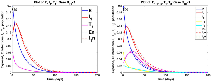
Fig. 6 (a) shows the comparison of the trajectories of the number (in percentages) of exposed ($En$), untreated infected ($I_{1}n$) population in stage 1 of infection for model (3.12) (no treatment) with the trajectories of the number of exposed (E), untreated infected ($I_1$) and treated infected ($T_1$) population in stage 1 of infection for model (2.1) (with treatment) for the case where $n=1$. Fig. 6 (b) shows the comparison of the trajectories of the number of exposed ($En$), untreated infected ($I_{1}n$) and ($I_{2}n$) population in stages 1 and 2 of infection, respectively, for model (3.12) with the trajectories of the number of exposed (E), untreated infected ($I_1$), ($I_2$) and treated infected ($T_1$), ($T_2$) populations in stages 1 and 2 of infection, respectively, for model (2.1) with the case $n=2$. It is clear from the graph that the introduction of treatment in the system reduces the number of exposed and infected individuals (that is, $E<En$, $I_1<I_{1}n$ and $I_2<I_{2}n$) after some days. The number of exposed and infected individuals tends to zero on the long run and the number of susceptible individuals tends to 1. In this case, $R_{01}=0.8885$, $R_{02}=0.9971$, $R_{T1}=0.8337$. and $R_{T2}=0.9255$. The graph of the solution $\left(S\left(t\right),E\left(t\right),I_1\left(t\right),\cdots ,I_n\left(t\right),R\left(t\right)\right)$ of system (3.12) converges to ${\tilde{P}}_0$ as $t\to \infty$. This confirms Corollary 5.5. Likewise, the graph of the solution $\left(S\left(t\right),E\left(t\right),I_1\left(t\right),\cdots ,I_n\left(t\right),T_1\left(t\right),\cdots ,T_n\left(t\right),R\left(t\right)\right)$ of system (2.1) converges to $P_0$ as $t\to \infty$. This confirms Theorem 5.4.

Fig. 6.

Graphs of comparison of deterministic trajectories of solution of system (2.1) and (3.12) for the cases where $n=1$ and $n=2$, respectively.

5.2. Existence and stability of endemic equilibrium $P_1$ in the presence of treatment

Theorem 5.6

The endemic equilibrium $P_1$ (given in (3.14)) of (2.1) exists if and only if $R_{T,n}>1$ and does not exist if $R_{T,n}<1$. It becomes disease-free (that is, $P_1=P_0$) if $R_{T,n}=1$.

Proof. It follows directly from (3.14) that ${\overline{S}}^{\text{*}}>0$, ${\overline{E}}^{\text{*}}>0$, ${\overline{I}}_k^{\text{*}}>0$, ${\overline{T}}_k^{\text{*}}>0$ and ${\overline{R}}^{\text{*}}>0$ for $k=\mathrm{1,2},\dots ,n$, if $R_{T,n}>1$. The result for the case where $R_{T,n}\le 1$ follows from (3.14). $■$

The following theorem gives the threshold for persistence of endemic (considered independent of the initial number of infection).

Theorem 5.7

The endemic equilibrium $P_1$ of the system (2.1) is globally stable in the feasible region $\mathcal{T}$ if $R_{T,n}>1and{f}_k>0,m_k>0,where{f}_{k}and{m}_{k}aregivenin(5.11).$

Proof. The existence of the endemic equilibrium $P_1$ follows from Theorem 5.6 if $R_{T,n}>1$. Assume $R_{T,n}>1$. Define the Lyapunov function $\overline{L}:{\mathbb{R}}_{2n+2}^{+}\to {\mathbb{R}}^{+}$ by

$$\overline{L}\left(S,I_1,\dots ,I_n,T_1,\dots ,T_n\right)=\left(S-{\overline{S}}^{\text{*}}-{\overline{S}}^{\text{*}}\ln \frac{S}{{\overline{S}}^{\text{*}}}\right)+{\overline{\varpi }}^{\text{*}}\left(E-{\overline{E}}^{\text{*}}-{\overline{E}}^{\text{*}}\ln \frac{E}{{\overline{E}}^{\text{*}}}\right)+\sum _{k=1}^n{\overline{\varphi }}_k^{\text{*}}\left(I_k-{\overline{I}}_k^{\text{*}}-{\overline{I}}_k^{\text{*}}\ln \frac{I_k}{{\overline{I}}_k^{\text{*}}}\right)+\sum _{k=1}^n{\overline{\theta }}_k^{\text{*}}\left(T_k-{\overline{T}}_k^{\text{*}}-{\overline{T}}_k^{\text{*}}\ln \frac{T_k}{{\overline{T}}_k^{\text{*}}}\right),$$ (5.8)

where ${\overline{\varpi }}^{\text{*}}$, ${\overline{\varphi }}_k^{\text{*}}$ and ${\overline{\theta }}_k^{\text{*}}$, $k=\mathrm{1,2},\dots ,n$, are positive constants defined by

$$\begin{array}{llll}{\overline{\varpi }}^{\text{*}}\hfill & =\hfill & 1,\hfill & \hfill \\ \left(\begin{array}{c}{\overline{\varphi }}_n^{\text{*}}\\ {\overline{\theta }}_n^{\text{*}}\end{array}\right)\hfill & =\hfill & \frac{\beta {\overline{S}}^{\text{*}}}{a_n{b}_n-{\tau }_n{\phi }_n}\left(\begin{array}{c}{h}_n{b}_n+{\tau }_n{\mathrm{\epsilon }}_n\\ h_n{\phi }_n+a_n{\mathrm{\epsilon }}_n\end{array}\right),\hfill & \hfill \\ \left(\begin{array}{c}{\overline{\varphi }}_{n-k}^{\text{*}}\\ {\overline{\theta }}_{n-k}^{\text{*}}\end{array}\right)\hfill & =\hfill & \frac{1}{a_{n-k}{b}_{n-k}-{\tau }_{n-k}{\phi }_{n-k}}\left[\left(\begin{array}{cc}{b}_{n-k}{\rho }_{n-k}& {\gamma }_{n-k}{\tau }_{n-k}\\ {\phi }_{n-k}{\rho }_{n-k}& {\gamma }_{n-k}{a}_{n-k}\end{array}\right)\left(\begin{array}{c}{\overline{\varphi }}_{n-k+1}^{\text{*}}\\ {\overline{\theta }}_{n-k+1}^{\text{*}}\end{array}\right)+\beta {\overline{S}}^{\text{*}}\left(\begin{array}{c}{h}_{n-k}{b}_{n-k}+{\tau }_{n-k}{\mathrm{\epsilon }}_{n-k}\\ h_{n-k}{\phi }_{n-k}+a_{n-k}{\mathrm{\epsilon }}_{n-k}\end{array}\right)\right],\text{for}k=\mathrm{1,2,3},\dots ,n-1,\hfill & \hfill \end{array}$$ (5.9)

and ${\left(\begin{array}{cc}{\overline{\varphi }}_1^{\text{*}}& {\overline{\theta }}_1^{\text{*}}\end{array}\right)}^{\top }$ reduces to

$$\left(\begin{array}{c}{\overline{\varphi }}_1^{\text{*}}\\ {\overline{\theta }}_1^{\text{*}}\end{array}\right)={\overline{S}}^{\text{*}}\frac{c}{\overline{\kappa }\pi }\left(\begin{array}{c}{R}_{T,n}\\ {\overline{R}}_{T,n}\end{array}\right),$$

where ${\overline{R}}_{T,n}$ is given in (5.7). It follows from (5.9) and (3.14) that ${\overline{\varpi }}^{\text{*}}c-{\overline{\varphi }}_1^{\text{*}}\pi =0$, ${\overline{\varphi }}_k^{\text{*}}{a}_k-{\overline{\varphi }}_{k+1}^{\text{*}}{\rho }_k-\beta {\overline{S}}^{\text{*}}{h}_k-{\tau }_k{\overline{\theta }}_k^{\text{*}}=0$, ${\overline{\theta }}_k^{\text{*}}{b}_k-{\overline{\theta }}_{k+1}^{\text{*}}{\gamma }_k-\beta {\overline{S}}^{\text{*}}{\mathrm{\epsilon }}_k-{\phi }_k{\overline{\varphi }}_k^{\text{*}}=0$ for $k=\mathrm{1,2},\dots ,n-1$, ${\overline{\varphi }}_n^{\text{*}}{a}_n-\beta {\overline{S}}^{\text{*}}{h}_n-{\tau }_n{\overline{\theta }}_n^{\text{*}}=0$ and ${\overline{\theta }}_n^{\text{*}}{b}_n-\beta {\overline{S}}^{\text{*}}{\mathrm{\epsilon }}_n-{\phi }_n{\overline{\varphi }}_n^{\text{*}}=0$.

The derivative of $\overline{L}$ computed along solution of (2.1) is

$$\begin{array}{c}\frac{d\overline{L}}{dt}=\text{Λ}-\text{Λ}\frac{{\overline{S}}^{\text{*}}}{S}-\mu S+\mu {\overline{S}}^{\text{*}}-\left(1-{\overline{\varpi }}^{\text{*}}\right)\beta S\stackrel{n}{\sum _{k=1}}\left(h_k{I}_k+{\mathrm{\epsilon }}_k{T}_k\right)-\left({\overline{\varpi }}^{\text{*}}c-{\overline{\varphi }}_1^{\text{*}}\pi \right)E-\stackrel{n-1}{\sum _{k=1}}\left({\overline{\varphi }}_k^{\text{*}}{a}_k-{\overline{\varphi }}_{k+1}^{\text{*}}{\rho }_k-\beta {\overline{S}}^{\text{*}}{h}_k-{\tau }_k{\overline{\theta }}_k^{\text{*}}\right)I_k\\ -\stackrel{n-1}{\sum _{k=1}}\left({\overline{\theta }}_k^{\text{*}}{b}_k-{\overline{\theta }}_{k+1}^{\text{*}}{\gamma }_k-\beta {\overline{S}}^{\text{*}}{\mathrm{\epsilon }}_k-{\phi }_k{\overline{\varphi }}_k^{\text{*}}\right)T_k-\left({\overline{\varphi }}_n^{\text{*}}{a}_n-\beta {\overline{S}}^{\text{*}}{h}_n-{\tau }_n{\overline{\theta }}_n^{\text{*}}\right)I_n-\left({\overline{\theta }}_n^{\text{*}}{b}_n-\beta {\overline{S}}^{\text{*}}{\mathrm{\epsilon }}_n-{\phi }_n{\overline{\varphi }}_n^{\text{*}}\right)T_n-{\overline{\varphi }}_1^{\text{*}}\pi {\overline{I}}_1^{\text{*}}\frac{E}{I_1}\\ -\stackrel{n}{\sum _{k=1}}\left({\overline{\varphi }}_k^{\text{*}}{\phi }_k{\overline{I}}_k^{\text{*}}\frac{T_k}{I_k}+{\overline{\theta }}_k^{\text{*}}{\tau }_k{\overline{T}}_k^{\text{*}}\frac{I_k}{T_k}\right)-\stackrel{n}{\sum _{k=2}}\left({\overline{\varphi }}_k^{\text{*}}{\rho }_{k-1}{\overline{I}}_k^{\text{*}}\frac{I_{k-1}}{I_k}+{\overline{\theta }}_k^{\text{*}}{\gamma }_{k-1}{\overline{T}}_k^{\text{*}}\frac{T_{k-1}}{T_k}\right)-{\overline{\varpi }}^{\text{*}}\beta {\overline{E}}^{\text{*}}\stackrel{n}{\sum _{k=1}}\left(h_k\frac{S{I}_k}{E}+{\mathrm{\epsilon }}_k\frac{S{T}_k}{E}\right),\\ +\stackrel{n}{\sum _{k=1}}\left({\overline{\varphi }}_k^{\text{*}}{a}_k{\overline{I}}_k^{\text{*}}+{\overline{\theta }}_k^{\text{*}}{b}_k{\overline{T}}_k\right)+{\overline{\varpi }}^{\text{*}}c{\overline{E}}^{\text{*}}.\end{array}$$

Define

$$s=\frac{S}{{\overline{S}}^{\text{*}}},e=\frac{E}{{\overline{E}}^{\text{*}}},i_k=\frac{I_k}{{\overline{I}}_k^{\text{*}}},\text{and}{t}_k=\frac{T_k}{{\overline{T}}_k^{\text{*}}}\text{for}k=\mathrm{1,2},\dots ,n,$$

$$\overline{C}=\text{Λ}+\mu {\overline{S}}^{\text{*}}+\stackrel{n}{\sum _{k=1}}\left({\overline{\varphi }}_k^{\text{*}}{a}_k{\overline{I}}_k^{\text{*}}+{\overline{\theta }}_k^{\text{*}}{b}_k{\overline{T}}_k\right)+{\overline{\varpi }}^{\text{*}}c{\overline{E}}^{\text{*}}.$$

We have

$$\begin{array}{l}\frac{d\overline{L}}{dt}=\overline{C}-\frac{\Lambda }{s}-\mu {\overline{S}}^{\ast }s-(1-{\overline{\varpi }}^{\ast })\beta {\overline{S}}^{\ast }s\sum _{k=1}^n\left(h_k{\overline{I}}_k^{\ast }{i}_k+{\mathrm{\epsilon }}_k{\overline{T}}_k^{\ast }{t}_k\right)-({\overline{\varpi }}^{\ast }c-{\overline{\varphi }}_1^{\ast }\pi ){\overline{E}}^{\ast }e\\ -\sum _{k=1}^{n-1}\left({\overline{\varphi }}_k^{\ast }{a}_k-{\overline{\varphi }}_{k+1}^{\ast }{\rho }_k-\beta {\overline{S}}^{\ast }{h}_k-{\tau }_k{\overline{\theta }}_k^{\ast }\right){\overline{I}}_k^{\ast }{i}_k-\sum _{k=1}^{n-1}\left({\overline{\theta }}_k^{\ast }{b}_k-{\overline{\theta }}_{k+1}^{\ast }{\gamma }_k-\beta {\overline{S}}^{\ast }{\mathrm{\epsilon }}_k-{\phi }_k{\overline{\varphi }}_k^{\ast }\right){\overline{T}}_k^{\ast }{t}_k-\left({\overline{\varphi }}_n^{\ast }{a}_n-\beta {\overline{S}}^{\ast }{h}_n-{\tau }_n{\overline{\theta }}_n^{\ast }\right){\overline{I}}_n^{\ast }{i}_n\\ -\left({\overline{\theta }}_n^{\ast }{b}_n-\beta {\overline{S}}^{\ast }{\mathrm{\epsilon }}_n-{\phi }_n{\overline{\varphi }}_n^{\ast }\right){\overline{T}}_n^{\ast }{t}_n-{\overline{\varphi }}_1^{\ast }\pi {\overline{E}}^{\ast }\frac{e}{i_1}-\sum _{k=1}^n\left({\overline{\varphi }}_k^{\ast }{\phi }_k{\overline{T}}_k^{\ast }\frac{t_k}{i_k}+{\overline{\theta }}_k^{\ast }{\tau }_k{\overline{I}}_k^{\ast }\frac{i_k}{t_k}\right)-\sum _{k=2}^n\left({\overline{\varphi }}_k^{\ast }{\rho }_{k-1}{\overline{I}}_{k-1}^{\ast }\frac{i_{k-1}}{i_k}+{\overline{\theta }}_k^{\ast }{\gamma }_{k-1}{\overline{T}}_{k-1}^{\ast }\frac{t_{k-1}}{t_k}\right)\\ -{\overline{\varpi }}^{\ast }\beta {\overline{S}}^{\ast }\sum _{k=1}^n\left(h_k{\overline{I}}_k^{\ast }\frac{s{i}_k}{e}+{\mathrm{\epsilon }}_k{\overline{T}}_k^{\ast }\frac{s{t}_k}{e}\right),\\ =-z\left(s+\frac{1}{s}-2\right)-\sum _{k=2}^n{g}_k(\frac{1}{s}+\frac{s{i}_k}{e}+\frac{e}{i_1}+\sum _{j=2}^k\frac{i_{j-1}}{i_j}-(k+2))-g_1\left(\frac{1}{s}+\frac{s{i}_1}{e}+\frac{e}{i_1}-3\right)\\ -\sum _{k=2}^n{f}_k(\frac{1}{s}+\frac{s{t}_k}{e}+\frac{e}{i_1}+\sum _{j=2}^k\frac{i_{j-1}}{i_j}+\frac{i_k}{t_k}-(k+3))-f_1\left(\frac{1}{s}+\frac{s{t}_1}{e}+\frac{e}{i_1}+\frac{i_1}{t_1}-4\right)-\sum _{k=1}^n{d}_k\left(\frac{i_k}{t_k}+\frac{t_k}{i_k}-2\right)\\ -\sum _{k=2}^n{m}_k(\frac{1}{s}+\frac{s{t}_k}{e}+\frac{e}{i_1}+\sum _{j=2}^k\frac{t_{j-1}}{t_j}+\frac{i_1}{t_1}-(k+3)),\end{array}$$ (5.10)

where

$$\begin{array}{c}z=\mu {\overline{S}}^{\ast },\\ d_k={\overline{\phi }}_k^{\ast }{\varphi }_k{\overline{T}}_k^{\ast },fork=\mathrm{1,2},\mathrm{...},n,\\ g_k={\overline{\varpi }}^{\ast }\beta {\overline{S}}^{\ast }{h}_k{\overline{I}}_k^{\ast },fork=\mathrm{1,2},\mathrm{...},n,\\ m_k={\overline{\theta }}_k^{\ast }{\gamma }_{k-1}{\overline{T}}_{k-1}^{\ast }-{\overline{\theta }}_{k+1}^{\ast }{\gamma }_k{\overline{T}}_k^{\ast },\text{for}k=\mathrm{2,3},\cdots ,n-1,\\ m_n={\overline{\theta }}_n^{\ast }{\gamma }_{n-1}{\overline{T}}_{n-1}^{\ast },\\ f_1={\overline{\varpi }}^{\ast }\beta {\overline{S}}^{\ast }{\mathrm{\epsilon }}_1{\overline{T}}_1^{\ast },\\ f_k={\overline{\theta }}_k^{\ast }{\tau }_k{\overline{I}}_k^{\ast }-d_k>0,\text{for}k=\mathrm{2,3},\cdots ,n,\\ \overline{C}=2z+\sum _{k=1}^n((2+k)g_k+(3+k)f_k+2d_k)+\sum _{k=2}^n(3+k)m_k.\end{array}$$ (5.11)

hence, from (5.10)–(5.11) and the fact that the arithmetic mean of a list of non-negative real numbers is greater than or equal to the geometric mean of the same list (Steele, 2004), it follows that $1={\left(s\frac{1}{s}\right)}^{\frac{1}{2}}\le \frac{1}{2}\left(s+\frac{1}{s}\right)$; $1={\left(\frac{1}{s}\frac{s{i}_1}{e}\frac{e}{i_1}\right)}^{\frac{1}{3}}\le \frac{1}{3}\left(\frac{1}{s}+\frac{s{i}_1}{e}+\frac{e}{i_1}\right)$; $1={\left(\frac{1}{s}\frac{s{t}_1}{e}\frac{e}{i_1}\frac{i_1}{t_1}\right)}^{\frac{1}{4}}\le \frac{1}{4}\left(\frac{1}{s}+\frac{s{t}_1}{e}+\frac{e}{i_1}+\frac{i_1}{t_1}\right)$; $1={\left(\frac{1}{s}\frac{s{i}_k}{e}\frac{e}{i_1}\prod _{j=2}^k\frac{i_{j-1}}{i_j}\right)}^{\frac{1}{k+2}}\le \frac{1}{k+2}\left(\frac{1}{s}+\frac{s{i}_k}{e}+\frac{e}{i_1}+\sum _{j=2}^k\frac{i_{j-1}}{i_j}\right)$; $1={\left(\frac{1}{s}\frac{s{t}_k}{e}\frac{e}{i_1}\frac{i_k}{t_k}\prod _{j=2}^k\frac{i_{j-1}}{i_j}\right)}^{\frac{1}{k+3}}\le \frac{1}{k+3}\left(\frac{1}{s}+\frac{s{t}_k}{e}+\frac{e}{i_1}+\frac{i_k}{t_k}+\sum _{j=2}^k\frac{i_{j-1}}{i_j}\right)$; $1={\left(\frac{1}{s}\frac{s{t}_k}{e}\frac{e}{i_1}\frac{i_1}{t_1}\prod _{j=2}^k\frac{t_{j-1}}{t_j}\right)}^{\frac{1}{k+3}}\le \frac{1}{k+3}\left(\frac{1}{s}+\frac{s{t}_k}{e}+\frac{e}{i_1}+\frac{i_1}{t_1}+\sum _{j=2}^k\frac{t_{j-1}}{t_j}\right)$ for $k=2,\dots ,n$, and $1={\left(\frac{i_k}{t_k}\frac{t_k}{i_k}\right)}^{\frac{1}{2}}\le \frac{1}{2}\left(\frac{i_k}{t_k}+\frac{t_k}{i_k}\right)$, for $k=\mathrm{1,2},\dots ,n$, and

$$\frac{d\overline{L}}{dt}\le 0.$$

Equality holds if and only if $S={\overline{S}}^{\text{*}}$, $E/{\overline{E}}^{\text{*}}=I_{j-1}/{\overline{I}}_{j-1}^{\text{*}}=I_j/{\overline{I}}_j^{\text{*}}=T_{j-1}/{\overline{T}}_{j-1}^{\text{*}}=T_j/{\overline{T}}_j^{\text{*}}=1$ for $j=\mathrm{2,3},\dots ,n$. Using (3.14) and the fact that $R\left(t\right)$ satisfies (2.1), it follows that $R\left(t\right)\to {\overline{R}}^{\text{*}}$ as $t\to \infty$. The largest invariant set of (2.1) contained in $\left\{{\left(S,E,I_1,\dots ,I_n,T_1,\dots ,T_n,R\right)}^{\top }\in \mathcal{T}:d\overline{L}/dt=0\right\}$ is the singleton $\left\{P_1\right\}$. By the LaSalle’s Invariance Principle (LaSalle, 1976), it follows that $P_1$ is globally stable in the feasible region if $R_{T,n}>1$ . $■$

The global stability of the endemic equilibrium ${\tilde{P}}_1$ of system (3.12) without treatment follows immediately from Theorem 5.7 by setting ${\tau }_k=0$ for all $k=\mathrm{1,2},\cdots ,n$. We state the theorem below without proof.

Corollary 5.8

The endemic equilibrium ${\tilde{P}}_1$ (given in (3.16)) of (3.12) is globally asymptotically stable if $R_{0,n}>1$.

5.2.1. Numerical results verifying the global stability of $P_1$ and effect of treatment

Using two infectious stages, we use the same values of parameters given in Table 3 except that we set $\beta =0.5,h_1=1.5,h_2=0.5,{\epsilon }_1=0.5,{\epsilon }_2=0.01,\mu =0.0125.$.

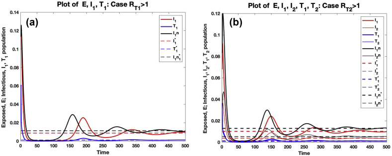
Fig. 7 (a) shows the comparison of the trajectories of the number of exposed ($En$), untreated infected ($I_{1}n$) individuals for model (3.12) with trajectories of the number of exposed (E), untreated infected ($I_1$) and treated infected ($T_1$) individuals for model (2.1) for the case where $n=1$ and $R_{T,1}>1$. Fig. 7 (b) shows the comparison of the trajectories of the number of exposed ($En$), untreated infected ($I_{1}n$), ($I_{2}n$) individuals for model (3.12) with trajectories of the number of exposed (E), untreated infected ($I_1$), ($I_2$), and treated infected ($T_1$), ($T_2$) individuals for model (2.1) for the case where $n=2$ and $R_{T,2}>1$. It is clear from the graph that the introduction of treatment in the system reduces the number of exposed and infected individuals (that is, $E<En$, $I_1<I_{1}n$ and $I_2<I_{2}n$) after some days. In this case, $R_{01}=1.7397$, $R_{02}=1.9549$, $R_{T1}=1.5934$. and $R_{T2}=1.7665$. The endemic equilibrium point for system (3.12) is (${\overline{S}}^{\text{*}}=0.5748,{\overline{E}}^{\text{*}}=0.0104,{\overline{I}}_1^{\text{*}}=0.0112,{\overline{R}}^{\text{*}}=0.1475$) for the case $n=1$ and (${\overline{S}}^{\text{*}}=0.5115,{\overline{E}}^{\text{*}}=0.0119,{\overline{I}}_1^{\text{*}}=0.0129,{\overline{I}}_2^{\text{*}}=0.0053,{\overline{R}}^{\text{*}}=0.1983$) for the case $n=2$. Likewise, the endemic equilibrium points for system (2.1) for cases $n=1$ and $n=2$ are (${\overline{S}}^{\text{*}}=0.6276,{\overline{E}}^{\text{*}}=0.0091,{\overline{I}}_1^{\text{*}}=0.0087,{\overline{T}}_1=0.0010,{\overline{R}}^{\text{*}}=0.1594$) and (${\overline{S}}^{\text{*}}=0.5661,{\overline{E}}^{\text{*}}=0.0106,{\overline{I}}_1^{\text{*}}=0.0101,{\overline{I}}_2^{\text{*}}=0.0037,{\overline{T}}_1^{\text{*}}=0.0012,{\overline{T}}_2^{\text{*}}=0.000842,{\overline{R}}^{\text{*}}=0.2240$), respectively. The graph of the solution $\left(S\left(t\right),E\left(t\right),I_1\left(t\right),\cdots ,I_n\left(t\right),R\left(t\right)\right)$ of system (3.12) converges to ${\tilde{P}}_1$ as $t\to \infty$. This confirms Corollary 5.8. Likewise, the graph of the solution $\left(S\left(t\right),E\left(t\right),I_1\left(t\right),\cdots ,I_n\left(t\right),T_1\left(t\right),\cdots ,T_n\left(t\right),R\left(t\right)\right)$ of system (2.1) converges to $P_1$ as $t\to \infty$. This confirms Theorem 5.7.

Fig. 7.

Graphs of comparison of deterministic trajectories of solution of system (2.1) and (3.12) for the cases where $n=1$ and $n=2$, with $R_{T,n}>1$.

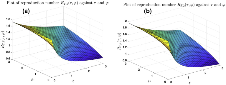
Fig. 8 (a) shows the graph of $R_{T,1}\equiv R_{T,1}\left(\tau ,\phi \right)$ against $\tau \equiv {\tau }_1$ and $\phi \equiv {\phi }_1$. Fig. 8 (b) shows the graph of $R_{T,2}\left(\tau ,\phi \right)$ against $\tau \equiv {\tau }_1={\tau }_2$ and $\phi \equiv {\phi }_1={\phi }_2$. The graphs show that for fixed φ, as more (less) treatment is introduced into the population, the number of secondary infection $R_{T,n}$ reduces (increases) until it approaches $R_{\infty ,n}$ ($R_{0,n}$), which is the least (highest) number of secondary infection that can be produced by an infected individuals when introduced into susceptible population. This is explained in Subsection 4.1. Also, the number of secondary infection $R_{T,n}$ increases to $R_{0,n}$ as individuals drop out of treatment. This is explained in 4.1, 4.2.

Fig. 8.

Effect of treatment and dropping out of treatment on the reproduction number for the cases $n=1$ and $n=2$, with $R_{T,n}>1$.

6. Derivation of stochastic model: effect of fluctuations and stability of disease-free equilibrium

In this section, we study the effect of noise on the transmission rates and infectivities, $\left\{\beta h_k,\beta {\mathrm{\epsilon }}_k\right\}$; the treatment rates $\left\{{\tau }_k\right\}$; the recovery rates $\left\{{\psi }_k\right\}$ and $\left\{{\eta }_k\right\}$ in stage k of untreated and treated individuals, respectively, for $k=\mathrm{1,2},\cdots ,n$. We assume the noise/external fluctiations in the system is caused by variability in the number of contacts between infected and susceptible individuals and such random variations can be modeled by a Gaussian white noise (Mendez et al., 2012). We also assume that fluctuations in the treatment rates may be caused by limited availability of drugs or effect of seasonality. This, in turn, causes fluctuations in the recovery rates. By allowing these rates to fluctuate about a mean value, we introduce external fluctuations in the model as follows:

$$\{\begin{array}{cccc}\beta & \equiv & \beta +\overline{\beta }\mathcal{C}\left(t\right),& \\ {\tau }_k& \equiv & {\tau }_k+{\overline{\tau }}_k{\mathcal{W}}_k\left(t\right),& \\ {\psi }_k& \equiv & {\psi }_k+{\overline{\psi }}_k{\mathcal{Z}}_k\left(t\right),& \\ {\eta }_k& \equiv & {\eta }_k+{\overline{\eta }}_k{\overline{\mathcal{Z}}}_k\left(t\right),\text{ for}k=\mathrm{1,2},\cdots ,n,& \end{array}$$ (6.1)

where ${\mathcal{C}}_k,{\mathcal{W}}_k,{\mathcal{Z}}_k$ and ${\overline{\mathcal{Z}}}_k$ are independent Gaussian noise terms with zero mean, and $\overline{\beta }>0$, ${\overline{\tau }}_k>0$, ${\overline{\psi }}_k>0$ and ${\overline{\eta }}_k>0$ are the noise intensities, a measure of the amplitude of fluctuations, for $k=\mathrm{1,2},\cdots ,n$. By substituting (6.1) into (2.1), we get a Langevin equation. The resulting equation is a stochastic differential equation. It is important to be able to interprete and evaluate the noise structure of this equation. The Itô approach on stochastic differential equation depends on Markovian and Martingale properties. These properties do not obey the traditional chain rule. Whereas, the Stratonovich approach obeys the traditional chain rule and allows white noise to be treated as a regular derivative of a Brownian or Wiener process. It has been suggested by several authors like West et al., Wong et al. (West et al., 1979; Wong & Zakai, 1965) that Stratonovich calculus is appropriate for Langevin equations with both internal and external noise. For this reason, by substituting (6.1) into (2.1), we extend the resulting equation to a Stratonovich stochastic model of the form

$$\begin{array}{l}dS=\left(\Lambda -\beta S\sum _{j=1}^n\left(h_j{I}_j+{\mathrm{\epsilon }}_j{T}_j\right)-\mu S\right)dt-S\sum _{j=1}^n\left({\sigma }_j{I}_j+{\overline{\sigma }}_j{T}_j\right)\circ d{C}_j\left(t\right),\\ dE=\left(\beta S\sum _{j=1}^n\left(h_j{I}_j+{\mathrm{\epsilon }}_j{T}_j\right)-(\pi +\mu )E\right)+S\sum _{j=1}^n\left({\sigma }_j{I}_j+{\overline{\sigma }}_j{T}_j\right)\circ d{C}_j\left(t\right),\\ d{I}_1=\left(\pi E-(\mu +{\delta }_1+{\rho }_1+{\tau }_1+{\psi }_1)I_1+{\phi }_1{T}_1\right)dt-{\overline{\tau }}_1{I}_1\circ d{W}_1\left(t\right)-{\overline{\psi }}_1{I}_1\circ d{Z}_1\left(t\right),\\ d{I}_k=\left({\rho }_{k-1}{I}_{k-1}-(\mu +{\delta }_k+{\rho }_k+{\tau }_k+{\psi }_k)I_k+{\phi }_k{T}_k\right)-{\overline{\tau }}_k{I}_k\circ d{W}_k\left(t\right)-{\overline{\psi }}_k{I}_k\circ d{Z}_k\left(t\right)dt,k=\mathrm{2,3},\mathrm{...},n,\\ d{T}_1=({\tau }_1{I}_1-(\mu +{\overline{\delta }}_1+{\gamma }_1+{\phi }_1+{\eta }_1)T_1)dt+{\overline{\tau }}_1{I}_1\circ d{W}_1\left(t\right)-{\overline{\eta }}_1{T}_1\circ d{\overline{Z}}_1\left(t\right),\\ d{T}_k=\left({\tau }_k{I}_k+{\gamma }_{k-1}{T}_{k-1}-(\mu +{\overline{\delta }}_k+{\gamma }_k+{\phi }_k+{\eta }_k)T_k\right)dt+{\overline{\tau }}_k{I}_k\circ d{W}_k\left(t\right)-{\overline{\eta }}_k{T}_k\circ d{\overline{Z}}_k\left(t\right),k=\mathrm{2,3},\mathrm{...},n,\\ dR=\left(\sum _{j=1}^n\left({\psi }_j{I}_j+{\eta }_j{T}_j\right)-\mu R\right)dt+\sum _{j=1}^n{\overline{\psi }}_j{I}_j\circ d{Z}_j\left(t\right)+\sum _{j=1}^n{\overline{\eta }}_j{T}_j\circ d{\overline{Z}}_j\left(t\right),\end{array}$$ (6.2)

where $\circ$ denotes the Stratonovich integral (Arnold, 1974); $C\left(t\right),W_i\left(t\right)$, $Z_i\left(t\right)$, ${\overline{Z}}_i\left(t\right)$, $i=\mathrm{1,2},\dots ,n$, are standard Wiener process on a filtered probability space ($\text{Ω},{\left({\mathcal{F}}_t\right)}_{t\ge 0},\mathbb{P}$); the initial process $x\left(t_0\right)=\left(S\left(t_0\right),E\left(t_0\right),I_1\left(t_0\right),\dots ,I_n\left(t_0\right),T_1\left(t_0\right),\dots ,T_n\left(t_0\right),R\left(t_0\right)\right)$ is ${\mathcal{F}}_{t_0}$ measurable and independent of $C\left(t\right)-C\left(t_0\right)$, $W_i\left(t\right)-W_i\left(t_0\right)$, $Z_i\left(t\right)-Z_i\left(t_0\right)$ and ${\overline{Z}}_i\left(t\right)-{\overline{Z}}_i\left(t_0\right)$, $i=\mathrm{1,2},\dots ,n$.

The Stratonovich dynamic model (6.2) is converted to its It$\hat{\text{o}}$’s equivalent (stated below) using the Stratonovich-It$\hat{\text{o}}$ conversion theorem given in Bernardi et al. (Bernardi, Madday, Blowey, Coleman, & Craig, 2001) and Kloeden et al. (Kloeden & Platen, 1995).

Theorem 6.1

The Itô stochastic differential equation having the same solution as the $2n+3$-dimensional Stratonovich stochastic differential equation (6.2) is given by

$$\begin{array}{l}dS=\left(\Lambda -\beta S\sum _{j=1}^n\left(h_j{I}_j+\mathrm{\epsilon }{T}_j\right)-\mu S+\frac{1}{2}S\sum _{j=1}^n{\left({\sigma }_j{I}_j+{\overline{\sigma }}_j{T}_j\right)}^2\right)dt-S\sum _{j=1}^n\left({\sigma }_j{I}_j+{\overline{\sigma }}_j{T}_j\right)d{C}_j\left(t\right),\\ dE=\left(\beta S\sum _{j=1}^n\left(h_j{I}_j+\mathrm{\epsilon }{T}_j\right)-(\pi +\mu )E-\frac{1}{2}S\sum _{j=1}^n{\left({\sigma }_j{I}_j+{\overline{\sigma }}_j{T}_j\right)}^2\right)+S\sum _{j=1}^n\left({\sigma }_j{I}_j+{\overline{\sigma }}_j{T}_j\right)d{C}_j\left(t\right),\\ d{I}_1=\left(\pi E-a_1{I}_1+{\phi }_1{T}_1+\frac{1}{2}\left({\overline{\tau }}_1^2+{\overline{\psi }}_1^2\right)I_1\right)dt-{\overline{\tau }}_1{I}_{1}d{W}_1\left(t\right)-{\overline{\psi }}_1{I}_{1}d{Z}_1\left(t\right),\\ d{I}_k=\left({\rho }_{k-1}{I}_{k-1}-a_k{I}_k+{\phi }_k{T}_k+\frac{1}{2}\left({\overline{\tau }}_k^2+{\overline{\psi }}_k^2\right)I_k\right)-{\overline{\tau }}_k{I}_{k}d{W}_k\left(t\right)-{\overline{\psi }}_k{I}_{k}d{Z}_k\left(t\right)dt,k=\mathrm{2,3},\mathrm{...},n,\\ d{T}_1=\left({\tau }_1{I}_1-b_1{T}_1+\frac{1}{2}\left(-{\overline{\tau }}_1^2{I}_1+{\overline{\eta }}_1^2{T}_1\right)\right)dt+{\overline{\tau }}_1{I}_{1}d{W}_1\left(t\right)-{\overline{\eta }}_1{T}_{1}d{\overline{Z}}_1\left(t\right),\\ d{T}_k=\left({\tau }_k{I}_k+{\gamma }_{k-1}{T}_{k-1}-b_k{T}_k+\frac{1}{2}\left(-{\overline{\tau }}_k^2{I}_k+{\overline{\eta }}_k^2{T}_k\right)\right)dt+{\overline{\tau }}_k{I}_{k}d{W}_k\left(t\right)-{\overline{\eta }}_k{T}_{k}d{\overline{Z}}_k\left(t\right),k=\mathrm{2,3},\mathrm{...},n,\\ dR=\left(\sum _{j=1}^n\left({\psi }_j{I}_j+{\eta }_j{T}_j\right)-\mu R-\frac{1}{2}\sum _{j=1}^n\left({\overline{\psi }}_j^2{I}_j+{\overline{\eta }}_j^2{T}_j\right)\right)dt+\sum _{j=1}^n\left({\overline{\psi }}_j{I}_{j}d{Z}_j\left(t\right)+{\overline{\eta }}_j{T}_{j}d{\overline{Z}}_j\left(t\right)\right).\end{array}$$ (6.3)

Proof. The proof follows using the Stratonovich-It$\hat{\text{o}}$ conversion theorem given in Bernardi et al. (Bernardi et al., 2001) and Kloeden et al. (Kloeden & Platen, 1995).

Following similar approach presented in Otunuga (Otunuga, 2018), we can show, using the function$\mathbf{V}\left(t,x\right)=\text{ln}\left(S+E+\sum _{j=1}^n\left(I_j+T_j\right)+R+e^{\text{Λ}}\right)$, that $\mathbb{L}\mathbf{V}<\mathbf{V}$ and $\underset{\left|x\right|>M}{\text{inf}}\mathbf{V}\left(t,x\right)\to \infty ,\text{ as}M\to \infty$, where $\mathbb{L}$ is a differential operator called the $\mathbb{L}$- operator defined by

$$\mathbb{L}\mathbf{V}\left(t,\mathbf{u}\right)=\frac{\partial \mathbf{V}\left(t,\mathbf{u}\right)}{\partial t}+\frac{\partial \mathbf{V}\left(t,\mathbf{u}\right)}{\partial \mathbf{u}}\mathbf{A}+\frac{1}{2}\text{trace}\left[{\mathbf{B}}^{\top }\frac{{\partial }^2\mathbf{V}\left(t,\mathbf{u}\right)}{\partial {\mathbf{u}}^2}\mathbf{B}\right]$$ (6.4)

where $\frac{\partial \mathbf{V}\left(t,\mathbf{u}\right)}{\partial \mathbf{u}}=\left(\frac{\partial \mathbf{V}\left(t,\mathbf{u}\right)}{\partial u_1},\dots ,\frac{\partial \mathbf{V}\left(t,\mathbf{u}\right)}{\partial u_{2n+3}}\right)$ and $\frac{{\partial }^2\mathbf{V}\left(t,\mathbf{u}\right)}{\partial {\mathbf{u}}^2}={\left(\frac{{\partial }^2\mathbf{V}\left(t,\mathbf{u}\right)}{\partial u_i\partial u_j}\right)}_{2n+3\times 2n+3}$. It follows from Theorem 3.5 of Khasminskii (Rafail, 2012) that there exists a solution $x\left(t\right)=\left(S\left(t\right),E\left(t\right),I_1\left(t\right),\dots ,I_n\left(t\right),T_1\left(t\right),\dots ,T_n\left(t\right),R\left(t\right)\right)$ of (6.3) which is an almost surely continuous stochastic process and is unique up to equivalence if $x\left(t_0\right)\in \mathcal{T}$ is independent of the processes $C_i\left(t\right)-C_i\left(t_0\right)$, $W_i\left(t\right)-W_i\left(t_0\right)$, $Z_i\left(t\right)-Z_i\left(t_0\right)$, ${\overline{Z}}_i\left(t\right)-{\overline{Z}}_i\left(t_0\right)$, $i=\mathrm{1,2},\cdots ,n$. The solution described above can be shown to be nonnegative and in the feasible region $\mathcal{T}$ using a similar idea presented in (Yang & Mao, 2013).

6.1. Equilibrium points and basic reproduction number in the presence of noise

The point $P_0$ defined in (3.1)–(3.2) is also the disease-free equilibrium of system (6.3). We calculate an equivalent of R_T,n in (3.6), denoted by ${\mathcal{R}}_{T,n}$ and derive threshold under which system (6.3) becomes disease-free on the long run. We first linearize the non-linear stochastic system about the disease-free equilibrium and study the stability of the solution of the linear system.

Define $\overline{\mathrm{\Psi }}={\left(\begin{array}{ccccc}S-\overline{\kappa }& E& I_1\dots I_n& T_1\dots T_n& R\end{array}\right)}^{\top }$. The linearization of (6.3) about the disease-free equilibrium $P_0$ results in

$$d\overline{\mathrm{\Psi }}=\mathcal{A}\overline{\mathrm{\Psi }}dt+\sum _{i=1}^n\left(G^{i}d{C}_i\left(t\right)+\overline{G^i}d{W}_i\left(t\right)+H^{i}d{Z}_i\left(t\right)+\overline{H^i}d{\overline{Z}}_i\left(t\right)\right)\overline{\mathrm{\Psi }},$$ (6.5)

where $\mathcal{A}=\left(\begin{array}{cccc}{\mathcal{A}}_{\mathrm{1,1}}& {\mathcal{A}}_{\mathrm{1,2}}& {\mathcal{A}}_{\mathrm{1,3}}& {\mathcal{A}}_{\mathrm{1,4}}\\ {\mathcal{A}}_{\mathrm{2,1}}& {\mathcal{A}}_{\mathrm{2,2}}& {\mathcal{A}}_{\mathrm{2,3}}& {\mathcal{A}}_{\mathrm{2,4}}\\ {\mathcal{A}}_{\mathrm{3,1}}& {\mathcal{A}}_{\mathrm{3,2}}& {\mathcal{A}}_{\mathrm{3,3}}& {\mathcal{A}}_{\mathrm{3,4}}\\ {\mathcal{A}}_{\mathrm{4,1}}& {\mathcal{A}}_{\mathrm{4,2}}& {\mathcal{A}}_{\mathrm{4,3}}& {\mathcal{A}}_{\mathrm{4,4}}\end{array}\right)$ with ${\mathcal{A}}_{\mathrm{1,1}}=A_{\mathrm{1,1}}$, ${\mathcal{A}}_{\mathrm{1,2}}=A_{\mathrm{1,2}}$, ${\mathcal{A}}_{\mathrm{1,3}}=A_{\mathrm{1,3}}$, ${\mathcal{A}}_{\mathrm{1,4}}=A_{\mathrm{1,4}}$, ${\mathcal{A}}_{\mathrm{2,1}}=A_{\mathrm{2,1}}$, ${\mathcal{A}}_{\mathrm{2,3}}=A_{\mathrm{2,3}}$, ${\mathcal{A}}_{\mathrm{2,4}}=A_{\mathrm{2,4}},{\mathcal{A}}_{\mathrm{3,1}}=A_{\mathrm{3,1}}$, ${\mathcal{A}}_{\mathrm{3,4}}=A_{\mathrm{3,4}}$, ${\mathcal{A}}_{\mathrm{4,1}}=A_{\mathrm{4,1}}$ and ${\mathcal{A}}_{\mathrm{4,4}}=A_{\mathrm{4,4}}$ defined in (5.1),

$$\begin{array}{llll}{\mathcal{A}}_{\mathrm{2,2}}\hfill & =\hfill & -\left(\begin{array}{ccccccc}{a}_1-\frac{{\overline{\tau }}_1^2+{\overline{\psi }}_1^2}{2}& 0& 0& 0& \dots & 0& 0\\ -{\rho }_1& a_2-\frac{{\overline{\tau }}_2^2+{\overline{\psi }}_2^2}{2}& 0& 0& \dots & 0& 0\\ 0& -{\rho }_2& a_3-\frac{{\overline{\tau }}_3^2+{\overline{\psi }}_3^2}{2}& 0& \dots & 0& 0\\ ⋮& ⋮& ⋮& ⋮& \ddots & ⋮& ⋮\\ 0& 0& \dots & \dots & \dots & -{\rho }_{n-1}& a_n-\frac{{\overline{\tau }}_n^2+{\overline{\psi }}_n^2}{2}\end{array}\right),\hfill & \hfill \\ {\mathcal{A}}_{\mathrm{3,3}}\hfill & =\hfill & -\left(\begin{array}{ccccccc}{b}_1-\frac{{\overline{\eta }}_1^2}{2}& 0& 0& 0& \dots & 0& 0\\ -{\gamma }_1& b_2-\frac{{\overline{\eta }}_2^2}{2}& 0& 0& \dots & 0& 0\\ 0& -{\gamma }_2& b_3-\frac{{\overline{\eta }}_3^2}{2}& 0& \dots & 0& 0\\ ⋮& ⋮& ⋮& ⋮& \ddots & ⋮& ⋮\\ 0& 0& \dots & \dots & \dots & -{\gamma }_{n-1}& b_n-\frac{{\overline{\eta }}_n^2}{2}\end{array}\right),\hfill & \hfill \end{array}$$

${\mathcal{A}}_{\mathrm{3,2}}={\mathcal{I}}_{\overline{\tau }}$, ${\mathcal{A}}_{\mathrm{4,2}}=\left(\begin{array}{cc}{\psi }_1-\frac{{\overline{\psi }}_1^2}{2}& {\psi }_2-\frac{{\overline{\psi }}_2^2}{2}\cdots {\psi }_n-\frac{{\overline{\psi }}_n^2}{2}\end{array}\right)$, ${\mathcal{A}}_{\mathrm{4,3}}=\left(\begin{array}{cc}{\eta }_1-\frac{{\overline{\eta }}_1^2}{2}& {\eta }_2-\frac{{\overline{\eta }}_2^2}{2}\cdots {\eta }_n-\frac{{\overline{\eta }}_n^2}{2}\end{array}\right)$, where.

${\mathcal{I}}_{\overline{\mathrm{\Psi }}}=\text{diag}\left({\overline{\mathrm{\Psi }}}_1,{\overline{\mathrm{\Psi }}}_2,\cdots ,{\overline{\mathrm{\Psi }}}_n\right)$, ${\mathcal{I}}_{\overline{\tau }}=\text{diag}\left({\tau }_1-\frac{{\overline{\tau }}_1^2}{2},{\tau }_2-\frac{{\overline{\tau }}_2^2}{2},\cdots ,{\tau }_n-\frac{{\overline{\tau }}_n^2}{2}\right)$, $a_k$ and $b_k$ are defined in (3.3), $G^i$, ${\overline{G}}^i$, $H^i$ and ${\overline{H}}^i$ are $2n+3\times 2n+3$ matrices with entries $G_{1,i+2}^i=-\overline{\kappa }{\sigma }_i$, $G_{1,n+i+2}^i=-\overline{\kappa }{\overline{\sigma }}_i$, $G_{2,i+2}^i=\overline{\kappa }{\sigma }_i$, $G_{2,n+i+2}^i=\overline{\kappa }{\overline{\sigma }}_i$, ${\overline{G^i}}_{i+2,i+2}=-{\overline{\tau }}_i$, ${\overline{G^i}}_{n+i+2,i+2}={\overline{\tau }}_i$, $H_{i+2,n+i+2}^i=-{\overline{\psi }}_i$, $H_{2n+3,i+2}^i={\overline{\psi }}_i$, ${\overline{H^i}}_{n+i+2,n+i+2}=-{\overline{\eta }}_i$, ${\overline{H^i}}_{2n+3,n+i+2}={\overline{\eta }}_i$, and zero otherwise for $j=\mathrm{1,2},\cdots ,n$. Define $\text{Ω}\left(t\right)=\mathbb{E}\left[\overline{\mathrm{\Psi }}\left(t\right)\right]$. The function $\text{Ω}\left(t\right)$ satisfies the differential equation

$$d\text{Ω}=\mathcal{A}\text{Ω}dt.$$ (6.6)

The characteristic polynomial of $\mathcal{A}$ can be expressed as

$$det\left(\mathcal{A}-\overline{r}{\mathcal{I}}_{2n+3\times 2n+3}\right)=-\left(\overline{r}+\mu \right)det\left(\overline{\mathcal{A}}-\overline{r}{\mathcal{I}}_{2n\times 2n}\right),$$ (6.7)

where $\overline{\mathcal{A}}$ is the matrix obtained be deleting the first row and column of $\mathcal{A}$ in (6.5), and $\overline{r}$ is the eigenvalue.

Using the idea presented in Mendez et al. (Mendez et al., 2012) and in Section 3.1.1, we calculate the reproduction number ${\mathcal{R}}_{T,n}$ with respect to the deterministic model (6.6) in the presence of treatment as

$$\begin{array}{cccc}{\mathcal{R}}_{T,n}& =& \frac{\overline{\kappa }\beta \pi }{c}\sum _{k=1}^n\left[\frac{{\tilde{u}}_k{h}_k+{\mathrm{\epsilon }}_k{\tilde{v}}_k}{\prod _{j=1}^k\left({\tilde{\alpha }}_j{\tilde{\beta }}_j-{\tilde{\tau }}_j{\phi }_j\right)}\right],& \end{array}$$ (6.8)

where

$$\begin{array}{l}{\tilde{\alpha }}_j=a_j-\frac{{\overline{\tau }}_j^2+{\overline{\psi }}_j^2}{2},\\ {\tilde{\beta }}_j=b_j-\frac{{\overline{\eta }}_j^2}{2},\\ {\tilde{\tau }}_j={\tau }_j-\frac{{\overline{\tau }}_j^2}{2},\\ {\tilde{u}}_k={\tilde{\beta }}_k{\rho }_{k-1}{\tilde{u}}_{k-1}+{\phi }_k{\gamma }_{k-1}{\tilde{v}}_{k-1},\\ {\tilde{v}}_k={\tilde{\tau }}_k{\rho }_{k-1}{\tilde{u}}_{k-1}+{\tilde{\alpha }}_k{\gamma }_{k-1}{\tilde{v}}_{k-1},\text{for}k=1,\cdots ,n,\end{array}$$

with ${\tilde{u}}_0=1$, ${\tilde{v}}_0=0$. We note here that the threshold ${\mathcal{R}}_{T,n}$ is nonnegative provided

$${\tilde{\tau }}_j\ge 0,{\tilde{\eta }}_j={\eta }_j-{\overline{\eta }}_j^2/2\ge 0,{\tilde{\psi }}_j={\psi }_j-{\overline{\psi }}_j^2/2\ge 0.$$ (6.9)

For the rest of this work, we assume condition (6.9) is satisfied.

Remark 6.1.1

We note here that the number ${\mathcal{R}}_{T,n}$ reduces to $R_{T,n}$ if ${\overline{\tau }}_j={\overline{\psi }}_j={\overline{\eta }}_j=0$ for all $j=\mathrm{1,2},\cdots ,n$.

Remark 6.1.2

Condition (6.9) indicates that the noise intensities ${\overline{\tau }}_j$, ${\overline{\psi }}_j$ and ${\overline{\eta }}_j$ must not exceed the rates $\sqrt{2{\tau }_j}$, $\sqrt{2{\psi }_j}$ and $\sqrt{2{\eta }_j}$, respectively, for the model to be well defined.

6.2. Effect of noise in the treatment, and recovery rates

In this section, we study the effect of fluctuations in the treatment and recovery rates.

6.2.1. Effect of noise in the treatment rates

Assuming condition (6.9) is satisfied, and ${\overline{\eta }}_j={\overline{\psi }}_j=0$ for $j=\mathrm{1,2},\cdots ,n$, we wish to study how the number of infection changes due to changes in the treatment intensity rates $\left\{{\overline{\tau }}_j\right\}$. Define $R_{T,n}\equiv R_{T,n}\left({\tau }_i\right)$ (given in (3.6)) and ${\mathcal{R}}_{T,n}\equiv {\mathcal{R}}_{T,n}\left({\tau }_i\right)$. It is easy to show that $R_{T,j}\left({\tau }_i-{\overline{\tau }}_i^2/2\right)={\mathcal{R}}_{T,j}\left({\tau }_i\right)$. As discussed in Subsection 4.1, the derivative $\frac{d{R}_{T,j}}{d{\tau }_i}\le 0$ if and only if $R_{T,j}({\tau }_i\to \infty )\le R_{T,j}({\tau }_i=0),\text{for}1\le i\le j\le n$, that is, $R_{T,j}\left({\tau }_i\right)$ is a decreasing function of ${\tau }_i$ if and only if $R_{T,j}({\tau }_i\to \infty \le R_{T,j}({\tau }_i=0),\text{for}1\le i\le j\le n$. It follows that $R_{T,j}\left({\tau }_i\right)\le {\mathcal{R}}_{T,j}\left({\tau }_i\right)$ provided $R_{T,j}({\tau }_i\to \infty )\le R_{T,j}({\tau }_i=0),\text{for}1\le i\le j\le n$. The same result follows for the case where ${\tau }_i\equiv \tau$ for all $i=\mathrm{1,2},\cdots ,n$, that is, $R_{T,n}\left(\tau \right)\le R_{T,n}\left(\tau -\frac{{\overline{\tau }}^2}{2}\right)={\mathcal{R}}_{T,n}\left(\tau \right)$ provided $R_{\infty ,n}<R_{0,n}$. An increase in the noise intensity in the treatment rate increases the number of secondary infection cases produced by a typical infective individual.

6.2.2. Effect of noise in the recovery rates of untreated infected individual

Assuming condition (6.9) is satisfied, and ${\overline{\tau }}_j={\overline{\eta }}_j=0$ for $j=\mathrm{1,2},\cdots ,n$. We wish to study how the number of infection changes due to changes in the untreated recovery intensity rates $\left\{{\overline{\psi }}_j\right\}$ of infected individual. Write ${\mathcal{R}}_{T,n}\equiv {\mathcal{R}}_{T,n}\left({\overline{\psi }}_1,\cdots ,{\overline{\psi }}_n\right)$ as a function of ${\left\{\overline{\psi }\right\}}_{j=1}^n$. Since the functions ${\tilde{g}}_j\left(t\right)=\frac{1}{\left(a_j-t^2/2\right)b_j-{\tau }_j{\phi }_j}$ and $g_j\left(t\right)=\frac{a_j-t^2/2}{\left(a_j-t^2/2\right)b_j-{\tau }_j{\phi }_j}$ are increasing function of t for $j=\mathrm{1,2},\cdots ,n$, and ${\mathcal{R}}_{T,n}\left({\overline{\psi }}_1,\cdots ,{\overline{\psi }}_n\right)$ can be expressed in terms of ${\tilde{g}}_j\left({\overline{\psi }}_j\right)$ and $g_j\left({\overline{\psi }}_j\right)$, it follows from the increasing property of $g_j\left({\overline{\psi }}_j\right)$ that ${\mathcal{R}}_{T,n}\equiv {\mathcal{R}}_{T,n}\left({\overline{\psi }}_1,\cdots ,{\overline{\psi }}_n\right)\ge {\mathcal{R}}_{T,n}\left(\mathrm{0,0},\cdots ,0\right)=R_{T,n}$. The higher the noise intensity in the untreated infected recovery rates, the higher the number of secondary infection cases produced by a typical infective individual.

6.2.3. Effect of noise in the recovery rates of treated infected individual

Assuming condition (6.9) is satisfied and ${\overline{\tau }}_j={\overline{\psi }}_j=0$ for $j=\mathrm{1,2},\cdots ,n$. By writing ${\mathcal{R}}_{T,n}\equiv {\mathcal{R}}_{T,n}\left({\overline{\eta }}_1,\cdots ,{\overline{\eta }}_n\right)$ as a function of ${\left\{\overline{\eta }\right\}}_{j=1}^n$, we wish to show that ${\mathcal{R}}_{T,n}>{\mathcal{R}}_{T,n}\left(0,\cdots ,0\right)=R_{T,n}$. Since the functions $\frac{1}{{\tilde{\alpha }}_j\left(b_j-\frac{{\overline{\eta }}_j^2}{2}\right)-{\tilde{\tau }}_j{\phi }_j}$ and $\frac{\left(b_i-\frac{{\overline{\eta }}_j^2}{2}\right)}{\left({\tilde{\alpha }}_j\left(b_j-\frac{{\overline{\eta }}_j^2}{2}\right)-{\tilde{\tau }}_j{\phi }_j\right)}$ are increasing function of ${\overline{\eta }}_j$ for $j=\mathrm{1,2},\cdots ,n$, it follows that ${\mathcal{R}}_{T,n}\equiv {\mathcal{R}}_{T,n}\left({\overline{\eta }}_1,\cdots ,{\overline{\eta }}_n\right)\ge {\mathcal{R}}_{T,n}\left(0,\cdots ,0\right)=R_{T,n}$, that is, as the noise intensity in the recovery rate ${\overline{\eta }}_j$ of treated infected individuals increases, the number of secondary infection cases produced by a typical infective individual increases.

6.2.4. Numerical analysis

We use the parameters presented in Table 3 to verify the results claimed in Sub1, 2, 3, 4, 5, 6.

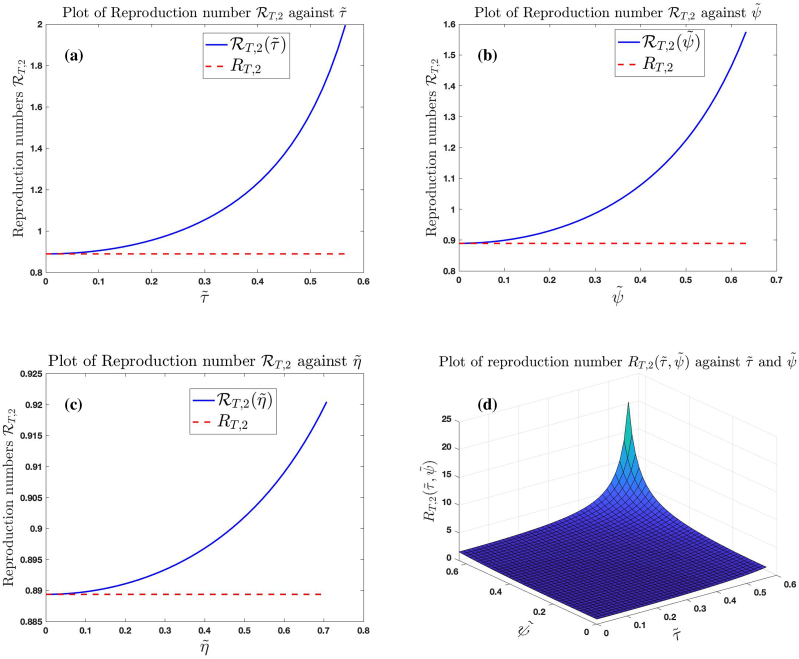
Fig. 9 (a), (b) and (c) show the graphs of ${\mathcal{R}}_{T,2}\equiv {\mathcal{R}}_{T,2}\left(\tilde{\tau }\right)$, ${\mathcal{R}}_{T,2}\equiv {\mathcal{R}}_{T,2}\left(\tilde{\psi }\right)$ and ${\mathcal{R}}_{T,2}\equiv {\mathcal{R}}_{T,2}\left(\tilde{\eta }\right)$ against $\tilde{\tau }$ (fixing $\tilde{\psi }=\tilde{\eta }=0)$), $\tilde{\psi }$ (fixing $\tilde{\tau }=\tilde{\eta }=0)$) and $\tilde{\eta }$ (fixing $\tilde{\tau }=\tilde{\psi }=0)$), respectively. Fig. 9 (d) shows the graph of ${\mathcal{R}}_{T,2}\equiv {\mathcal{R}}_{T,2}\left(\tilde{\tau },\tilde{\psi }\right)$ against $\tilde{\tau }$ and $\tilde{\psi }$. The trajectories of these graphs suggest that the higher the intensity of noise in the treatment rate, recovery rates of untreated and treated infected individuals, the higher the number of secondary infections produced by an infected individuals when introduced into a susceptible population.

Fig. 9.

Effect of noise on treatment rates and recovery rates of untreated and treated infected individuals for the case $n=2$.

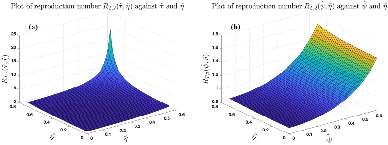
Fig. 10 (a) and (b) show the graphs of ${\mathcal{R}}_{T,2}\equiv {\mathcal{R}}_{T,2}\left(\tilde{\tau },\tilde{\eta }\right)$ against $\tilde{\tau }$ and $\tilde{\eta }$ and ${\mathcal{R}}_{T,2}\equiv {\mathcal{R}}_{T,2}\left(\tilde{\psi },\tilde{\eta }\right)$ against $\tilde{\psi }$ and $\tilde{\eta }$. The trajectories of these graphs suggests that the higher the intensity of noise in the treatment rate, recovery rates of untreated and treated infected individuals, the higher the number of secondary infections produced by an infected individuals when introduced into a susceptible population.

Fig. 10.

Effect of noise on treatment rates and recovery rates of untreated and treated infected individuals for the case $n=2$.

6.3. Stability of infection-free equilibrium $P_0$ of (6.3)

In this section, we discuss conditions for stability of the infection-free equilibrium $P_0$ of (6.3) in the presence of noise. We study the conditions for stochastic stability of the disease-free equilibrium $P_0$ of the linear associated system (6.5) and later use Theorem A.2 in (Tornatore et al., 2005) to extend the result to that of the nonlinear system (6.3).

Theorem 6.2

Assume condition (6.9) is satisfied. The real part of all eigenvalues of $\mathcal{A}$ is negative if ${\mathcal{R}}_{T,n}<1$.

Proof. The proof follows from (6.9) and Theorem 5.1 by setting $a_j\equiv a_j-\frac{{\overline{\tau }}_j^2+{\overline{\psi }}_j^2}{2}$, $b_j\equiv b_j-\frac{{\overline{\eta }}_j^2}{2}$, ${\tau }_j\equiv {\tau }_j-\frac{{\overline{\tau }}_j^2}{2}$, ${\psi }_j\equiv {\psi }_j-\frac{{\overline{\psi }}_j^2}{2}$, and ${\eta }_j\equiv {\eta }_j-\frac{{\overline{\eta }}_j^2}{2}$ into matrix A in (5.1). $■$

Writing the system of non-linear stochastic differential equation (6.3) in terms of $\overline{\mathrm{\Psi }}$ reduces to

$$\begin{array}{l}d{\overline{\Psi }}_1=\left(-\beta ({\overline{\Psi }}_1+\overline{\kappa })\sum _{j=1}^n\left(h_j{\overline{\Psi }}_{j+2}+{\mathrm{\epsilon }}_j{\overline{\Psi }}_{n+j+2}\right)-\mu {\overline{\Psi }}_1+\frac{1}{2}({\overline{\Psi }}_1+\overline{\kappa })\sum _{j=1}^n{\left({\sigma }_j{\overline{\Psi }}_{j+2}+{\overline{\sigma }}_j{\overline{\Psi }}_{n+j+2}\right)}^2\right)dt\\ -({\overline{\Psi }}_1+\overline{\kappa })\sum _{j=1}^n\left({\sigma }_j{\overline{\Psi }}_{j+2}+{\overline{\sigma }}_j{\overline{\Psi }}_{n+j+2}\right)d{C}_j\left(t\right),\\ d{\overline{\Psi }}_2=\left(\beta ({\overline{\Psi }}_1+\overline{\kappa })\sum _{j=1}^n\left(h_j{\overline{\Psi }}_{j+2}+{\mathrm{\epsilon }}_j{\overline{\Psi }}_{n+j+2}\right)-c{\overline{\Psi }}_2-\frac{1}{2}({\overline{\Psi }}_1+\overline{\kappa })\sum _{j=1}^n{\left({\sigma }_j{\overline{\Psi }}_{j+2}+{\overline{\sigma }}_j{\overline{\Psi }}_{n+j+2}\right)}^2\right)\\ +({\overline{\Psi }}_1+\overline{\kappa })\sum _{j=1}^n\left({\sigma }_j{\overline{\Psi }}_{j+2}+{\overline{\sigma }}_j{\overline{\Psi }}_{n+j+2}\right)d{C}_j\left(t\right),\\ d{\overline{\Psi }}_3=\left({\sigma }_E{\overline{\Psi }}_2-a_1{\overline{\Psi }}_3+{\overline{\Psi }}_1{\overline{\Psi }}_{n+3}+\frac{1}{2}({\overline{\tau }}_1^2+{\overline{\psi }}_1^2){\overline{\Psi }}_3\right)dt-{\overline{\tau }}_1{\overline{\Psi }}_{3}d{W}_1\left(t\right)-{\overline{\psi }}_1{\overline{\Psi }}_{3}d{Z}_1\left(t\right),\\ d{\overline{\Psi }}_{k+2}=\left({\rho }_{k-1}{\overline{\Psi }}_{k+1}-a_k{\overline{\Psi }}_{k+2}+{\overline{\Psi }}_k{\overline{\Psi }}_{n+k+2}+\frac{1}{2}({\overline{\tau }}_k^2+{\overline{\psi }}_k^2){\overline{\Psi }}_{k+2}\right)dt-{\overline{\tau }}_k{\overline{\Psi }}_{k+2}d{W}_k\left(t\right)-{\overline{\psi }}_k{\overline{\Psi }}_{k+2}d{Z}_k\left(t\right),\text{for},\\ d{\overline{\Psi }}_{n+3}=({\tau }_1{\overline{\Psi }}_3-b_1{\overline{\Psi }}_{n+3}+\frac{1}{2}(-{\overline{\tau }}_1^2{\overline{\Psi }}_3+{\overline{\eta }}_1^2{\overline{\Psi }}_{n+3})dt+{\overline{\tau }}_1{\overline{\Psi }}_{3}d{W}_1(t)-{\overline{\eta }}_1{\overline{\Psi }}_{n+3}d{\overline{Z}}_1(t)\\ d{\overline{\Psi }}_{n+k+2}=\left({\tau }_k{\overline{\Psi }}_{k+2}+{\gamma }_{k-1}{\overline{\Psi }}_{n+k+1}-b_k{\overline{\Psi }}_{n+k+2}+\frac{1}{2}(-{\overline{\tau }}_k^2{\overline{\Psi }}_{k+2}+{\overline{\eta }}_k^2{\overline{\Psi }}_{n+k+2}\right)dt+{\overline{\tau }}_k{\overline{\Psi }}_{k+2}d{W}_1\left(t\right)-{\overline{\eta }}_k{\overline{\Psi }}_{n+k+2}d{\overline{Z}}_k\left(t\right),\text{for},\\ d{\overline{\Psi }}_{2n+3}=\left(\sum _{j=1}^n\left({\psi }_j{\overline{\Psi }}_{j+2}+{\eta }_j{\overline{\Psi }}_{n+j+2}\right)-\mu {\overline{\Psi }}_{2n+3}-\frac{1}{2}\sum _{j=1}^n\left({\overline{\psi }}_j^2{\overline{\Psi }}_{j+2}+{\overline{\eta }}_j^2{\overline{\Psi }}_{n+j+2}\right)\right)dt+\sum _{j=1}^n\left({\overline{\psi }}_j{\overline{\Psi }}_{j+2}d{Z}_j\left(t\right)+{\overline{\eta }}_j{\overline{\Psi }}_{n+j+2}d{\overline{Z}}_j\left(t\right)\right),\end{array}$$ (6.10)

for $k=2,\cdots ,n$, where $a_k$ and $b_k$ are defined in (3.3).

Let F and $\mathcal{G}$ be the drift and diffusion coefficients of the linear system (6.5), respectively, and f and g the drift and diffusion coefficients of the non-linear system (6.10), respectively. We give a theorem concerning the global stability of the disease-free equilibrium point $P_0$ by showing that Theorems A.1 and A.2 of Tornatore et al., (2005) is satisfied with respect to systems (6.5) and (6.10).

Theorem 6.3

The disease-free equilibrium $P_0$ of the system (6.3) is globally asymptotically stable in the feasible region $\mathcal{T}$ if ${\mathcal{R}}_{T,n}<1$.

To prove this, we first show that if ${\mathcal{R}}_{T,n}<1$, the trivial solution $\overline{\mathrm{\Psi }}=0$ of the linear stochastic differential equation (6.5) is assymptotically stable and later show that the drift and diffusion coefficients $f\left(t,\overline{\mathrm{\Psi }}\right)$ and $g\left(t,\overline{\mathrm{\Psi }}\right)$, respectively, of the nonlinear system (6.10) satisfy the inequality

$$\Vert f\left(t,\overline{\mathrm{\Psi }}\right)-F\left(t,\overline{\mathrm{\Psi }}\right)\Vert +\Vert g\left(t,\overline{\mathrm{\Psi }}\right)-\mathcal{G}\left(t,\overline{\mathrm{\Psi }}\right)\Vert <\xi \Vert \overline{\mathrm{\Psi }}\Vert$$ (6.11)

in a sufficiently small neighbourhood of $\overline{\mathrm{\Psi }}=0$, with a sufficiently small constant ξ.

Proof. If ${\mathcal{R}}_{T,n}<1$, it follows from Theorem 6.2 that the real part of all eigenvalues of $\mathcal{A}$ is negative. Hence, there exist a diagonal matrix $\mathrm{\Upsilon }$ (with positive diagonal entries, say, $r_1,r_2,\cdots ,r_{2n+3}$ ) and a real number $\hat{z}>0$ such that $s^{\top }\left(\mathrm{\Upsilon }\mathcal{A}+{\mathcal{A}}^{\top }\mathrm{\Upsilon }\right)s\le -\hat{z}{s}^{\top }s$ for every nonzero vector $s\in {\mathbb{R}}^{2n+3}$ (see relation $I_{25}$ of (Plemmons, 1977)) . Let $\overline{\mathrm{\Psi }}={\left({\overline{\mathrm{\Psi }}}_1,{\overline{\mathrm{\Psi }}}_2,\dots ,{\overline{\mathrm{\Psi }}}_{2n+3}\right)}^{\top }$ be a vector satisfying the linear system (6.5) and define $V:[0,T]\times {\mathbb{R}}^{2n+3}\to {\mathbb{R}}^{+}$ by

$$V\left(t,\overline{\mathrm{\Psi }}\right)={\overline{\mathrm{\Psi }}}^T\mathrm{\Upsilon }\overline{\mathrm{\Psi }}.$$

Let $\hat{s}=\underset{1\le j\le n}{\text{max}}\left\{{\sigma }_j^2,{\overline{\sigma }}_j^2,{\overline{\tau }}_j,{\overline{\psi }}_j,{\overline{\eta }}_j\right\}$ such that $r_1=r_2=\frac{\hat{z}}{10{\overline{\kappa }}^2\hat{s}}$, $r_{j+2}=r_{n+j+2}=r_{2n+3}=\frac{\hat{z}}{10\hat{s}}$, for $j=\mathrm{1,2},\cdots ,n$. Using (6.4), the $\mathbb{L}$-operator defined in (6.4) satisfies

$$\begin{array}{c}\mathbb{L}V\left(t,\overline{\mathrm{\Psi }}\right)={\overline{\mathrm{\Psi }}}^{\top }\left(\mathrm{\Upsilon }\mathcal{A}+{\mathcal{A}}^{\top }\mathrm{\Upsilon }\right)\overline{\mathrm{\Psi }}+{\overline{\mathrm{\Psi }}}^{\top }\stackrel{n}{\sum _{i=1}}\left(G^{i\top }\mathrm{\Upsilon }{G}^i+{\overline{G^i}}^{\top }\mathrm{\Upsilon }\overline{G^i}+H^{i\top }\mathrm{\Upsilon }{H}^i+{\overline{H^i}}^{\top }\mathrm{\Upsilon }\overline{H^i}\right)\overline{\mathrm{\Psi }}\\ \le -\hat{z}{\overline{\mathrm{\Psi }}}^{\top }\overline{\mathrm{\Psi }}+{\overline{\mathrm{\Psi }}}^{\top }\stackrel{n}{\sum _{i=1}}\left(G^{i\top }\mathrm{\Upsilon }{G}^i+{\overline{G^i}}^{\top }\mathrm{\Upsilon }\overline{G^i}+H^{i\top }\mathrm{\Upsilon }{H}^i+{\overline{H^i}}^{\top }\mathrm{\Upsilon }\overline{H^i}\right)\overline{\mathrm{\Psi }}\\ =-\hat{z}\sum _{j=1}^{2n+3}{\overline{\mathrm{\Psi }}}_j^2+\sum _{j=1}^n\left(\left(r_1+r_2\right){\overline{\kappa }}^2{\sigma }_j^2+\left(r_{j+2}+r_{n+j+2}\right){\overline{\tau }}_j^2+r_{2n+3}{\overline{\psi }}_j^2\right){\overline{\mathrm{\Psi }}}_{j+2}^2\\ +\stackrel{n}{\sum _{j=1}}\left(\left(r_1+r_2\right){\overline{\kappa }}^2{\overline{\sigma }}_j^2+r_{j+2}{\overline{\psi }}_j^2+\left(r_{2n+3}+r_{n+j+2}\right){\overline{\eta }}_j^2\right){\overline{\mathrm{\Psi }}}_{n+j+2}^2\\ \le -\hat{z}\stackrel{2n+3}{\sum _{j=1}}{\overline{\mathrm{\Psi }}}_j^2+\frac{z}{2}\stackrel{n}{\sum _{j=1}}{\overline{\mathrm{\Psi }}}_{j+2}^2+\frac{\hat{z}}{2}\stackrel{n}{\sum _{j=1}}{\overline{\mathrm{\Psi }}}_{n+j+2}^2=-z{\overline{\mathrm{\Psi }}}_1^2-z{\overline{\mathrm{\Psi }}}_2^2-\frac{z}{2}\stackrel{n}{\sum _{j=1}}{\overline{\mathrm{\Psi }}}_{j+2}^2-\frac{\hat{z}}{2}\stackrel{n}{\sum _{j=1}}{\overline{\mathrm{\Psi }}}_{n+j+2}^2<-\frac{\hat{z}}{2}{\overline{\mathrm{\Psi }}}^{\top }\overline{\mathrm{\Psi }}.\end{array}$$

Let $r_l$ and $r_u$ be $\text{min}\left\{r_1,\dots ,r_{2n+3}\right\}$ and $\text{max}\left\{r_1,\dots ,r_{2n+3}\right\}$, respectively. Then $r_l{\Vert \overline{\mathrm{\Psi }}\Vert }^2\le V\left(t,\overline{\mathrm{\Psi }}\right)\le r_u{\Vert \overline{\mathrm{\Psi }}\Vert }^2$. It follows from Theorem A.1 of Tornatore et al., (2005) that the trivial solution $\overline{\mathrm{\Psi }}=0$ of (6.5) is asymptotically stable. We deduce from this result that if the initial condition (in $\mathcal{T}$) of system (6.5) is near 0, then the solution $\left(S\left(t\right),E\left(t\right),I_1\left(t\right),\cdots ,I_n\left(t\right),T_1\left(t\right),\cdots ,T_n\left(t\right),R\left(t\right)\right)$ approaches $P_0$ on the long run if ${\mathcal{R}}_{T,n}<1$. To prove the global stability of the solution $\overline{\mathrm{\Psi }}=0$ of (6.10) (equivalent to the disease-free equilibrium $P_0$ of (6.3)), we choose $\xi >0$ sufficiently small in a neighbourhood of $\overline{\mathrm{\Psi }}=0$ so that $\left|\overline{\mathrm{\Psi }}\right|<\xi$ and $|f\left(t,\overline{\mathrm{\Psi }}\right)-F\left(t,\overline{\mathrm{\Psi }}\right)|+|g\left(t,\overline{\mathrm{\Psi }}\right)-\mathcal{G}\left(t,\overline{\mathrm{\Psi }}\right)|$ reduces to

$$\sqrt{2{\left(\beta {\overline{\mathrm{\Psi }}}_1\stackrel{n}{\sum _{j=1}}\left(h_j{\overline{\mathrm{\Psi }}}_{j+2}+{\mathrm{\epsilon }}_j{\overline{\mathrm{\Psi }}}_{n+j+2}\right)-\frac{1}{2}\left({\overline{\mathrm{\Psi }}}_1+\overline{\kappa }\right)\stackrel{n}{\sum _{j=1}}\left({\sigma }_j{\overline{\mathrm{\Psi }}}_{j+2}+{\overline{\sigma }}_j{\overline{\mathrm{\Psi }}}_{n+j+2}\right)\right)}^2}+\sqrt{2{\overline{\mathrm{\Psi }}}_1^2{\left(\stackrel{n}{\sum _{j=1}}\left({\sigma }_j{\overline{\mathrm{\Psi }}}_{j+2}+{\overline{\sigma }}_j{\overline{\mathrm{\Psi }}}_{n+j+2}\right)\right)}^2}$$

$$\le \sqrt{2}\left({\overline{\mathrm{\Psi }}}_1^2\left(\frac{1}{2}\stackrel{n}{\sum _{j=1}}\beta \left(h_j^2+{\mathrm{\epsilon }}_j^2\right)+\left({\sigma }_j^2+{\overline{\sigma }}_j^2\right)\right)+\frac{1}{2}\left(\xi +\overline{\kappa }\right)\stackrel{n}{\sum _{j=1}}\left({\sigma }_j{\overline{\mathrm{\Psi }}}_{j+2}^2+{\overline{\sigma }}_j{\overline{\mathrm{\Psi }}}_{n+j+2}^2\right)+\frac{1}{2}\left(\beta +1\right)\stackrel{n}{\sum _{j=1}}\left({\overline{\mathrm{\Psi }}}_{j+2}^2+{\overline{\mathrm{\Psi }}}_{n+j+2}^2\right)\right)$$

$$\le \overline{h}\left|\overline{\mathrm{\Psi }}\right|,$$

where $\overline{h}=\xi \sqrt{2}\underset{1\le j\le n}{\text{max}}\left\{\frac{1}{2}\sum _{i=1}^n\beta \left(h_i^2+{\mathrm{\epsilon }}_i^2\right)+\left({\sigma }_j^2+{\overline{\sigma }}_j^2\right),\beta +1,\left(\mathrm{\xi }+\overline{\kappa }\right){\sigma }_j,\left(\mathrm{\xi }+\overline{\kappa }\right){\overline{\sigma }}_j\right\}.$ The global stability result follows from Theorem A.2 of (Tornatore et al., Vetro).

6.4. Numerical verification of global stability of infection-free equilibrium points for the stochastic model

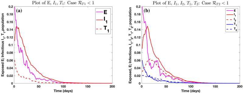
Fig. 11 (a) shows the trajectories of E, $I_1$ and $T_1$ satisfying model (6.3) for the case where $n=1$ and ${\mathcal{R}}_{T,1}<1$. Fig. 11 (b) shows the trajectory of E, $I_1$, $I_2$, $T_1$, $T_2$ satisfying model (6.3) for the case where $n=2$ and ${\mathcal{R}}_{T,2}<1$. In this case, ${\mathcal{R}}_{T1}=0.8056$ and ${\mathcal{R}}_{T2}=0.8908$.

Fig. 11.

Graphs of stochastic trajectories of solution of system (6.3) for the cases where $n=1$ and $n=2$, respectively, and ${\mathcal{R}}_{T,n}<1$.

Handling Editor: Dr Y. Shao

References

- Arnold L. Wiley; New York: 1974. Stochastic differential equations: Theory and applications. [Google Scholar]
- Bernardi C., Madday Y., Blowey J.F., Coleman J.P., Craig A.W. Springer-Verlag Berlin Heidelberg; 2001. Theory and numerics of differential equations. [Google Scholar]
- Biggerstaff M., Jhung M., Kamimoto L., Balluz L., Finelli L. Self-reported influenza-like Illness and Receipt of influenza antiviral drugs During the 2009 pandemic, United States, 2009-2010. American Journal of Public Health. 2012;102(10):21–26. doi: 10.2105/AJPH.2012.300651. [DOI] [PMC free article] [PubMed] [Google Scholar]
- Birrell P.J., Presanis A.M., De Angelis D. MRC Biostatistics Unit; 2012. The CASCADE collaboration. Multi-state models of HIV progression in homosexual men: An application to the CASCADE collaboration. Technical report. [Google Scholar]
- Diekmann O., Heesterbeek J.A.P., Metz J.A.J. On the definition and the computation of the basic reproduction ratio iR0in models for infectious diseases in heterogeneous populations. Journal of Mathematical Biology. 1990;28:365. doi: 10.1007/BF00178324. [DOI] [PubMed] [Google Scholar]
- Driessche P.V., Watmough J. Reproduction numbers and sub-threshold endemic equilibria for compartmental models of disease transmission. Mathematical Biosciences. 2002;180 doi: 10.1016/s0025-5564(02)00108-6. 29-48. [DOI] [PubMed] [Google Scholar]
- Etbaigha F., Willms A.R., Poljak Z. An SEIR model of influenza A virus infection and reinfection within a farrow-to-finish swine farm. PLoS One. 2018;13(9) doi: 10.1371/journal.pone.0202493. [DOI] [PMC free article] [PubMed] [Google Scholar]
- Feng Z., Towers S., Yang Y. Modeling the Effects of Vaccination and Treatment on pandemic influenza. The AAPS Journal. 2011;13(3):427–436. doi: 10.1208/s12248-011-9284-7. [DOI] [PMC free article] [PubMed] [Google Scholar]
- Gani R., Hughes H., Fleming D., Griffin T., Jolyon Medlock, Leach S. Potential impact of antiviral drug use during influenza pandemic. Emerging Infectious Diseases. 2005;11(9):1355–1362. doi: 10.3201/eid1109.041344. [DOI] [PMC free article] [PubMed] [Google Scholar]
- Godoy P., Romero A., Núria S., Nuria T., Mireia J., Ana M. The Working Group on Surveillance of Severe Influenza Hospitalized Cases in Catalonia. Influenza vaccine effectiveness in reducing severe outcomes over six influenza seasons, a case-case analysis, Spain. Euro Surveillance. 2018;23(43) doi: 10.2807/1560-7917.ES.2018.23.43.1700732. 2010/11 to 2015/16. [DOI] [PMC free article] [PubMed] [Google Scholar]
- Grassly N., Fraser C. Seasonal infectious disease epidemiology. Proceedings of the Royal Society Series B. 2006;273:2541–2550. doi: 10.1098/rspb.2006.3604. [DOI] [PMC free article] [PubMed] [Google Scholar]
- Hollingsworth T.D., Anderson R.M., Fraser C. HIV-1 transmission, by stage of infection. The Journal of Infectious Diseases. 2008;198(5):687–693. doi: 10.1086/590501. Sep 1. [DOI] [PubMed] [Google Scholar]
- Hu H., Nigmatulina K., Eckhoff P. Vol. 244. Mathematical Biosciences; 2013. The scaling of contact rates with population density for the infectious disease models. 125-134. [DOI] [PubMed] [Google Scholar]
- Huo H., Chen R., Wang X. Modelling and stability of HIV/AIDS epidemic model with treatment. Applied Mathematical Modelling. 2016;40:6550–6559. [Google Scholar]
- Kloeden P.E., Platen E. Springer-Verlag; New York: 1995. Numerical solution of stochastic differential equations. [Google Scholar]
- Korobeinikov A. Global properties of SIR and SEIR epidemic models with multiple parallel infectious stages. Bulletin of Mathematical Biology. 2009;71:75–83. doi: 10.1007/s11538-008-9352-z. [DOI] [PubMed] [Google Scholar]
- Kretzschmar M.E., Schim van der Loeff M.F., Birrell P.J., Angelis D.D., Coutinho R.A. Prospects of elimination of HIV with test-and-treat strategy. Proceedings of the National Academy of Sciences. 2013;110(39):15538–15543. doi: 10.1073/pnas.1301801110. [DOI] [PMC free article] [PubMed] [Google Scholar]
- LaSalle J.P. SIAM; Philadelphia: 1976. The stability of dynamical systems: Regional conference series in applied mathematics. [Google Scholar]
- Liu J., Zhang T. Global stability for a tuberculosis model. Mathematical and Computer Modelling. 2011;54:836–845. [Google Scholar]
- Li J., Xiao Y., Zhang F., Yang Y. An algebraic approach to proving the global stability of a class of epidemic models. Nonlinear Analysis: Real World Applications. 2012;13:2006–2016. [Google Scholar]
- Melesse D.Y., Gumel A.B. Global asymptotic properties of an SEIRS model with multiple infectious stages. Journal of Mathematical Analysis and Applications. 2010;366:202–217. [Google Scholar]
- Mendez V., Campos D., Horsthemke W. Stochastic fluctuations of the transmission rate in the susceptible-infected-susceptible epidemic model. Physical Review E. 2012;86 doi: 10.1103/PhysRevE.86.011919. [DOI] [PubMed] [Google Scholar]
- Mummert A., Otunuga O. Parameter identification for a stochastic SEIRS epidemic model: Case study influenza. Journal of Mathematical Biology. 2019;79(2):1–25. doi: 10.1007/s00285-019-01374-z. [DOI] [PMC free article] [PubMed] [Google Scholar]
- Murphy S.L., Xu J., Kochanek K.D., Arias E. Mortality in the United States, 2017. NCHS Data Brief. 2018;328 November. [PubMed] [Google Scholar]
- Otunuga O.M. Global stability of nonlinear stochastic SEI epidemic model. International Journal of Stochastic Analysis. 2017;2017:1–7. Article ID 6313620. [Google Scholar]
- Otunuga O.M. Global stability for a 2n+1 dimensional HIV/AIDS epidemic model with treatments. Mathematical Biosciences. 2018;299:138–152. doi: 10.1016/j.mbs.2018.03.013. [DOI] [PubMed] [Google Scholar]
- Plemmons R.J. M-matrix characterizations. I–Nonsingular M-matrices. Linear Algebra and Its Applications. 1977;18(2):175–188. [Google Scholar]
- Qiu Z., Feng Z. Transmission dynamics of an influenza model with vaccination and antiviral treatment. Bulletin of Mathematical Biology. 2010;72:1–33. doi: 10.1007/s11538-009-9435-5. [DOI] [PubMed] [Google Scholar]
- Rafail K. 2nd ed. Springer-Verlag Berlin Heidelberg; 2012. Stochastic stability of differential equations; p. 66. [Google Scholar]
- Roosa K., Chowell G. Assessing parameter identifiability in compartmental dynamic models using a computational approach: Application to infectious disease transmission models. Theoretical Biology and Medical Modelling. 2019;16(1):1–15. doi: 10.1186/s12976-018-0097-6. [DOI] [PMC free article] [PubMed] [Google Scholar]
- Steele J.M. Cambridge University Press; 2004. The Cauchy-Schwarz master class: An introduction to the art of mathematical inequalities. MAA problem books series. [Google Scholar]
- Tokars J.I., Olsen S.J., Reed C. Seasonal incidence of symptomatic influenza in the United States. Clinical Infectious Diseases. 2018;66(10):1511–1518. doi: 10.1093/cid/cix1060. [DOI] [PMC free article] [PubMed] [Google Scholar]
- Tornatore E., Buccellato S.M., Vetro P. Stability of a stochastic SIR system. Physica A. 2005;354(1–4):111–126. [Google Scholar]
- West B.J., Bulsara A.R., Lindenberg K., Seshadri V., Shuler K.E. Stochastic processes with non-additive fluctuations: I. Itô and Stratonovich calculus and the effects of correlations. Physica A. 1979;97(2):211–233. [Google Scholar]
- Wong E., Zakai M. On the convergence of ordinary integrals to stochastic integrals. The Annals of Mathematical Statistics. 1965;36(5):1560–1564. [Google Scholar]
- Yang Q., Mao X. Extinction and recurrence of multi-group SEIR epidemic models with stochastic perturbations. Nonlinear Analysis: Real World Applications. 2013;14:1434–1456. [Google Scholar]