

Summary
Inhibitory neurons, which play a critical role in decision-making models, are often simplified as a single pool of non-selective neurons lacking connection specificity. This assumption is supported by observations in primary visual cortex: inhibitory neurons are broadly tuned in vivo, and show non-specific connectivity in slice. Selectivity of excitatory and inhibitory neurons within decision circuits, and hence the validity of decision-making models, is unknown. We simultaneously measured excitatory and inhibitory neurons in posterior parietal cortex of mice judging multisensory stimuli. Surprisingly, excitatory and inhibitory neurons were equally selective for the animal’s choice, both at the single cell and population level. Further, both cell types exhibited similar changes in selectivity and temporal dynamics during learning, paralleling behavioral improvements. These observations, combined with modeling, argue against circuit architectures assuming non-selective inhibitory neurons. Instead, they argue for selective subnetworks of inhibitory and excitatory neurons that are shaped by experience to support expert decision-making.
Graphical Abstract
eTOC blurb:
Najafi et al. studied selectivity of mouse excitatory and inhibitory neurons during decision making. Selectivity is equally strong in the two cell types, and emerges gradually during learning. These data, along with theoretical models, argue that selective subnetworks support decision-making.
Introduction
In many decisions, noisy evidence is accumulated over time to support a categorical choice. At the neural level, a number of models can implement evidence accumulation (Wang, 2002; Machens et al., 2005; Bogacz et al., 2006; Lo and Wang, 2006; Wong and Wang, 2006; Beck et al., 2008; Lim and Goldman, 2013; Rustichini and Padoa-Schioppa, 2015; Mi et al., 2017). Although these circuit models successfully reproduc key characteristics of behavioral and neural data during perceptual decision-making, their empirical evaluation has been elusive, mainly due to the challenge of identifying inhibitory neurons reliably and in large numbers in behaving animals. Inhibition, which constitutes an essential component of these models, is usually provided by a single pool of inhibitory neurons receiving broad input from all excitatory neurons (non-selective inhibition, Deneve et al., 1999; Wang, 2002; Mi et al., 2017).
The assumption of non-selective inhibition in theoretical models was, perhaps, motivated by empirical studies examining connectivity and tuning of inhibitory neurons. Many studies in primary visual cortex report that inhibitory neurons have, on average, broader tuning curves than excitatory neurons for visual stimulus features such as orientation (Sohya et al., 2007; Niell and Stryker, 2008; Liu et al., 2009; Kerlin et al., 2010; Bock et al., 2011; Hofer et al., 2011; Atallah et al., 2012; Chen et al., 2013; Znamenskiy et al., 2018), spatial frequency (Niell and Stryker, 2008; Kerlin et al., 2010; Znamenskiy et al., 2018), and temporal frequency (Znamenskiy et al., 2018). Broad tuning in inhibitory neurons has been mostly attributed to their dense (Hofer et al., 2011; Packer and Yuste, 2011), functionally unbiased inputs from surrounding excitatory neurons (Kerlin et al., 2010; Bock et al., 2011; Hofer et al., 2011). Excitatory neurons, by contrast, show relatively sharp selectivity to stimulus features (Sohya et al., 2007; Niell and Stryker, 2008; Ch'ng and Reid, 2010; Kerlin et al., 2010; Hofer et al., 2011; Isaacson and Scanziani, 2011; Lee et al., 2016), reflecting their specific, non-random connectivity (Yoshimura et al., 2005; Ch'ng and Reid, 2010; Hofer et al., 2011; Ko et al., 2011; Cossell et al., 2015; Ringach et al., 2016).
Based on relatively weak tuning of inhibition, one might assume that inhibition in decision circuits is non-specific. However, the overall picture from experimental observations is more nuanced than the original studies suggest. First, some V1 studies report tuning of inhibitory neurons that is on par with excitatory neurons (Ma et al., 2010; Runyan et al., 2010), likely supported by targeted connectivity with excitatory neurons (Yoshimura and Callaway, 2005). Strong tuning of inhibitory neurons has also been reported in primary auditory cortex (Moore and Wehr, 2013). Further, in frontal and parietal areas, interneurons can distinguish go vs. no-go responses (Allen et al., 2017) and trial outcome (Pinto and Dan, 2015). Similarly, hippocampal interneurons have strong selectivity for the stimulus (Lowett-Brown 2017), and the animal’s location (Maurer et al., 2006; Ego-Stengel and Wilson, 2007).
This selectivity of inhibitory neurons in a wealth of areas and conditions argues that the assumption of non-selective interneurons in decision-making models must be revisited. Here, we aimed to evaluate this directly. We compared selectivity of inhibitory and excitatory neurons in posterior parietal cortex (PPC) in mice during pereptual decisions. Surprisingly, we found that excitatory and inhibitory neurons are equally choice-selective. Our modeling argued that these observations imply selective subnetworks, a network architecture supporting enhanced decoding in the presence of noise. Finally, during learning, selectivity of excitatory and inhibitory neurons increased in parallel. These results constrain decision-making models, and argue that in decision areas, subnetworks of selective inhibitory neurons emerge during learning and are engaged during expert decisions.
Results
To test how excitatory and inhibitory neurons coordinate during decision-making, we measured neural activity in transgenic mice trained to report decisions about the repetition rate of a sequence of multisensory events by licking to a left or right waterspout (Figure 1A; Figure S1A). Trials consisted of simultaneous clicks and flashes, generated randomly (via a Poisson process) at rates that from 5-27 Hz over 1000 ms (Brunton et al., 2013; Odoemene et al., 2017). Mice reported whether event rates were high or low compared to a category boundary (16 Hz) learned from experience. Decisions depended strongly on stimulus rate: performance was at chance when the stimulus rate was at the category boundary, and was better at rates further from the category boundary (Figure 1B). Choice depended on current stimulus strength, previous choice outcome (Hwang et al., 2017), and time elapsed since the previous trial (Figure S1B).
Figure 1. Simultaneous imaging of inhibitory and excitatory populations during decision-making.

A. Behavioral apparatus. Multisensory stimuli are presented via a visual display and a speaker. To initiate trials, mice lick the middle waterspout. To report decisions about stimulus rate, mice lick left/right spouts. Objective: 2-photon microscope used to image neural activity through an implanted window. B. Psychometric function showing the fraction of trials in which the mouse chose “high” as a function of stimulus rate. Dots: mean (10 mice). Line: Logit regression model (glmfit.m); mean across mice. Shaded area: standard deviation of the fit across mice. Dashed vertical line: category boundary (16Hz). C, Average image (10,000 frames). Left: green channel, GCaMP6f. Middle: red channel, tdTomato. Right: merge of left and middle. Cyan circles: GCaMP6f-expressing neurons identified as inhibitory. D, Example neurons identified by the Constrained Nonnegative Matrix Factorization algorithm (Methods) (arrow: inhibitory neuron). Left: raw ΔF/F traces. Middle: de-noised traces. Right: inferred spiking activity. Imaging was not performed during inter-trial intervals; traces from 13 consecutive trials are concatenated; dashed lines: trial onset. E, Example session; 568 neurons. Rows: trial-averaged inferred spiking activity of a neuron (frame resolution: 32.4ms). Neurons are sorted based on timing of peak activity. To ensure peaks were not driven by noisy fluctuations, we first computed trial-averaged activity using 50% of trials for each neuron. We then identified the peak-activity time for the trial-averaged response. Finally, these peak times determined the plotting order for the trial-averaged activity for the remaining 50% of trials. This cross-validated approach ensured that the tiling appearance of peak activities was not due to the combination of sorting and false-color-plotting. Red ticks at right: inhibitory neurons (n=45). Red vertical lines: trial events; Duration between events varied across trials; to make trial-averaged traces, traces were separately aligned to each trial event, and then averaged across trials. Next, averaged traces (each aligned to a different trial event) were concatenated. Vertical blue lines: border between the concatenated traces. F, Trial-averaged inferred spiking activity of 4 excitatory (top) and 4 inhibitory (bottom) neurons, for ipsi- (black) and contralateral (green) choices (mean±standard error (SEM); ~250 trials per session). G, Inferred spiking activity for excitatory (blue) and inhibitory (red) neurons. Example mouse; mean±SEM across days (n=46). Each point corresponds to an average over trials and neurons. Inferred spiking activity was downsampled by averaging over three adjacent frames (Methods). H, Distribution of inferred spiking activity 0-97ms before choice (averaged over three frames) for all mice/sessions (41,723 excitatory; 5,142 inhibitory). I, Inferred spiking activity 0-97ms before the choice (averaged over three frames) for individual mice (mean±SEM across days).
We imaged excitatory and inhibitory neural activity by injecting a viral vector containing the calcium indicator GCaMP6f to layer 2/3 of mouse Posterior Parietal Cortex (PPC; Harvey et al., 2012; Funamizu et al., 2016; Goard et al., 2016; Morcos and Harvey, 2016; Hwang et al., 2017; Song et al., 2017). Mice expressed the red fluorescent protein tdTomato transgenically in all GABAergic inhibitory neurons (Methods). We used a two-channel two-photon microscope to record the activity of all neurons, a subset of which were identified as inhibitory (Figure 1C). This allowed us to measure the activity of excitatory and inhibitory populations in the same animal.
To detect neurons and extract calcium signals, we leveraged an algorithm that simultaneously identifies neurons, de-noises the fluorescence signal and de-mixes signals from spatially overlapping components (Pnevmatikakis et al., 2016; Giovannucci et al., 2018) (Figure 1D middle). The algorithm also estimates spiking activity for each neuron, yielding, for each frame, a number that is related to the spiking activity during that frame (Figure 1D right). We refer to this number as “inferred spiking activity”, acknowledging that estimating spikes from calcium signals is challenging (Chen et al., 2013). Analyses were performed on inferred spiking activity. To identify inhibitory neurons, we developed a method to correct for bleed-through from the green to the red channel (Methods). We identified a subset of GCaMP6f-expressing neurons as inhibitory based on signal intensity (red channel) and spatial correlation between red and green channels (Figure 1C right, cyan circles). Inhibitory neurons constituted 11% of the population, within the range of the previous reports (Beaulieu, 1993; Gabbott et al., 1997; Rudy et al., 2011; Sahara et al., 2012), but on the lower side due to our desire to be conservative in assigning neurons to the inhibitory pool (Methods).
Confirming previous reports (Funamizu et al., 2016; Morcos and Harvey, 2016; Runyan et al., 2017), we observed that the activity of individual neurons peaked at time points spanning the trial (Figure 1E,F). Diverse temporal dynamics were evident in both cell types (Figure 1E,F) and did not appreciably differ between the two (Figure S2). The magnitude of inferred spiking activity was significantly different for inhibitory vs. excitatory neurons throughout the trial (Figure 1G; t-test, p<0.001). Just before the choice (97 ms, average of 3 frames), this difference was clear (Figure 1H) and significant for all mice (Figure 1I, t-test; p<0.001). Differences in GCaMP expression levels and calcium buffering between excitatory and inhibitory neurons, as well as how spiking activity is inferred (Methods), makes a direct estimate of the underlying firing rates challenging (Kwan and Dan, 2012). Nevertheless, the significant difference in the inferred spiking activity between excitatory and inhibitory neurons provides additional evidence that we successfully identified two separate neural populations.
Individual excitatory and inhibitory neurons are similarly choice-selective
To assess the selectivity of individual excitatory and inhibitory neurons for decision outcome, we performed receiver operating characteristic (ROC) analysis (Green and Swets, 1966) on single-neuron responses. A neuron was identified as “choice-selective” if the area under the ROC curve (AUC) differed significantly (p<0.05) from a shuffled distribution (Figure S3A; Methods), indicating that the neural activity differed significantly ipsi- vs. contralateral choices (Figure 2A).
Figure 2. Single-cell and pairwise analyses argue for non-random connections between excitatory and inhibitory neurons.

All panels: blue/red indicate excitatory/inhibitory neurons, respectively. A, Distribution of AUC values (area under the curve) of an ROC analysis for distinguishing choice from the activity of single neurons in an example session. Data correspond to the 97 ms window preceding choice (285 excitatory and 29 inhibitory neurons). Values larger than 0.5 indicate preference for ipsilateral choice; values smaller than 0.5 indicate preference for contralateral choice. Shaded areas: significant AUC values (compared to a shuffle distribution). Distributions were smoothed (moving average, span=5). 5 inhibitory and 24 excitatory neurons (17% and 8%, respectively) were significantly choice selective. B, ROC analysis on 97 ms non-overlapping time windows. Vertical axis: fraction of excitatory or inhibitory neurons with significant choice selectivity; example mouse; mean±SEM across days (n = 45 days). C, Fraction of excitatory and inhibitory neurons that are significantly choice-selective (0-97 ms before the choice) summarized for each mouse; mean±SEM across days (n = 45, 48, 7, 35 sessions per mouse). Star indicates significant difference (t-test; p<0.05); see also Figure S3D. Fraction selective neurons at 0-97ms before choice (median across mice): excitatory: 13%; inhibitory: 16%, (~6 inhibitory and 43 excitatory neurons with significant choice selectivity per session). D, ROC analysis for 97 ms non-overlapping time windows. Time course of normalized choice selectivity (defined as twice the absolute deviation of AUC from chance, given explicitly by 2*∣AUC-0.5∣) for excitatory and inhibitory neurons in an example mouse; mean±SEM across days, n = 45 sessions. E, Average of normalized choice selectivity for excitatory and inhibitory neurons (0-97 ms before choice) summarized for each mouse; mean±SEM across days. “Shuffled” denotes AUC was computed using shuffled trial labels.
The fraction of choice-selective neurons (Figure 2B) and the magnitude of choice selectivity (Figure 2D) gradually increased over the trial, peaking just after the animal reported its choice. Importantly, excitatory and inhibitory neurons were similar in terms of the fraction of choice-selective neurons (Figure 2B,C; Figure S3B,C), as well as the magnitude and time course (Figure 2D,E) of choice selectivity. When we restricted the analysis to excitatory and inhibitory neurons with similar spiking activity, the cell types remained equally selective for the animal’s choice (Figure S3D).
To assess whether neurons reflected the animal’s choice or the sensory stimulus, we compared choice selectivity on correct vs. error trials. For most neurons, choice selectivity on correct trials was similar to that on error trials, resulting in a positive correlation of the two quantities across neurons (Figure S3E). Positive correlations indicate that most neurons reflect the impending choice more so than the sensory stimulus that informed it (Methods). Variability across mice in the strength of this correlation may indicate that the balance of sensory vs. choice signals within individual neurons varied across subjects (perhaps due to imaged subregions within the window, Figure S3E right). Importantly, however, within each subject, this correlation was very similar for excitatory vs. inhibitory neurons (Figure S3E), suggesting that the tendency for neurons to be modulated by the choice vs. the stimulus was similar in excitatory and inhibitory neurons.
The existence of task-modulated inhibitory neurons has been reported elsewhere (Maurer et al., 2006; Ego-Stengel and Wilson, 2007; Lovett-Barron et al., 2014; Pinto and Dan, 2015; Allen et al., 2017; Kamigaki and Dan, 2017), but importantly, here choice selectivity was similarly strong in excitatory and inhibitory neurons, both in fraction and magnitude. This was at odds with the commonly accepted assumption of non-specific inhibition in theoretical studies (Deneve et al., 1999; Wang, 2002; Mi et al., 2017), and surprising given the numerous empirical findings suggesting broad tuning and weakly specific connectivity in inhibitory neurons (Sohya et al., 2007; Niell and Stryker, 2008; Liu et al., 2009; Kerlin et al., 2010; Bock et al., 2011; Hofer et al., 2011; Isaacson and Scanziani, 2011; Packer and Yuste, 2011; Atallah et al., 2012; Chen et al., 2013). This observation was a first hint that specific functional subnetworks, preferring either ipsi- or contralateral choices, exist within the inhibitory population, just like the excitatory population (Yoshimura and Callaway, 2005; Znamenskiy et al., 2018).
Choice is decoded with equal accuracy from both excitatory and inhibitory populations
While individual inhibitory neurons could distinguish the animal’s choice as well as excitatory ones, overall choice selectivity in single neurons was small (Figure 2E). To further evaluate the neurons’ discriminability, we trained linear classifiers (support vector machine, SVM; Hofmann et al., 2008) to predict the mouse’s choice from the single-trial population activity (cross-validated; L2 penalty; see Methods).
We first tested all neurons imaged simultaneously in a single session (Figure 3A, left), training the classifier separately at each timepoint (97 ms bins). Classification accuracy gradually grew after stimulus onset and peaked at the time of the choice (Figure 3B, black). The ability of the entire population of PPC neurons to predict the choice confirms previous observations (Funamizu et al., 2016; Goard et al., 2016; Morcos and Harvey, 2016; Driscoll et al., 2017). Our overall classification accuracy was in the same range as these studies, and, as in those studies, was high although many individual neurons in the population were only weakly selective (Figure. 2A).
Figure 3. Linear classifiers can predict the animal’s choice with equal accuracy from the activity of excitatory or inhibitory populations.

A, Schematic of decoding choice from all neurons (left), only excitatory (middle), subsampled to the same number as inhibitory neurons, and only inhibitory (right). A linear SVM assigns weights of different magnitude (indicated by lines of different thickness) to each neuron in the population. B, Top: classification accuracy of decoders trained on all neurons (black), subsampled excitatory neurons (blue), and inhibitory neurons (red) (cross-validated; decoders trained on every 97ms time bin; example session; mean±SEM across 50 cross-validated samples). Data are aligned to the animal’s choice (black dotted line). Unsaturated lines : performance on shuffled trials. Bottom: distribution of stimulus onset, offset, go tone, and reward occurrence for the example session above. C, Classification accuracy (0-97 ms before the choice, mean±SEM across days) for real (saturated) and shuffled (unsaturated) data. D, Absolute value of weights for excitatory and inhibitory neurons in decoders trained on all neurons; mean±SEM across days. E, Distribution of classifier weights (decoder training time: 0-97 ms before the choice) for excitatory and inhibitory neurons. Neurons from all mice pooled (42,019 excitatory and 5,172 inhibitory neurons). Shading: standard error. F, Absolute value of weights in the classifier (0-97 ms before choice) for excitatory vs. inhibitory neurons. Mean±SEM across days. Star: p<0.05, t-test. G, Schematic of decoding choice from a population of subsampled excitatory neurons (top) vs. a population with half inhibitory and half excitatory neurons (bottom). H, Classifier accuracy of populations including only excitatory (blue) or half inhibitory, half excitatory neurons (magenta); example session. Classifier trained at each moment in the trial. Traces show mean±SEM (50 cross-validated samples). I, Summary of each mouse (mean±SEM across days) for the decoders (0-97 ms before the choice).
We then examined classifier accuracy for excitatory and inhibitory populations, subsampling the excitatory population so that the total number of neurons was matched (Figure 3A, middle). Overall classification accuracy was reduced due to the smaller population size, but performance was still well above chance (Figure 3B, blue trace). Finally, we included all inhibitory neurons (Figure 3A, right). Classification accuracy of inhibitory neurons was well above chance and was very similar to that of excitatory neurons (Figure 3B, red and blue traces overlap; Figure S4: additional example sessions). Similar classification accuracy for excitatory and inhibitory populations was observed in all subjects (Figure 3C). Excitatory and inhibitory populations were equally choice selective even when the analysis was performed on raw calcium traces (Figure S5).
Our analysis may have obscured a difference between excitatory and inhibitory neurons because we evaluated their performance separately, rather than considering how these neurons are leveraged collectively in a classifier with both cell types. To test this, we examined a classifier that was trained on all neurons (Figure 3A left; Figure 3B black), and compared classifier weights assigned to excitatory vs. inhibitory neurons. The weight magnitudes of excitatory and inhibitory neurons were matched for the entire trial (Figure 3D), and the distributions of weights was very similar (Figures 3E, F). The comparable classifier weights for excitatory and inhibitory neurons argues that these cell types are similarly informative for choice.
We next tested whether excitatory and inhibitory populations can be decoded more accurately from a mixed population. This could occur, for example, if the excitatory-inhibitory correlations were weak relative to excitatory-excitatory and inhibitory-inhibitory correlations (Panzeri et al., 1999; Averbeck et al., 2006; Moreno-Bote et al., 2014). To assess this, we trained the classifier on a population with half excitatory and half inhibitory neurons (Figure 3G bottom), and compared its accuracy with a classifier trained on a population of the same size that consisted only of excitatory neurons (Figure 3G top). Classification accuracy was similar for both decoders (Figure 3H,I), arguing that a mixed population offers no major advantage to decoding.
We next trained new classifiers to evaluate whether population activity reflected additional task features. First, the population activity was somewhat informative about previous trial choice (Figure S6A), in agreement with previous studies (Morcos and Harvey, 2016; Hwang et al., 2017; Akrami et al., 2018); but also see (Zhong et al., 2018). Excitatory and inhibitory populations were similarly selective for previous choice (Figure S6A). The population activity was also somewhat informative about whether the stimulus was above or below the category boundary (Figure S6B). Again, excitatory and inhibitory populations were similarly selective (Figure S6B). Finally, population activity was strongly selective for trial outcome (reward vs. lack of reward; Figure S6C). Excitatory and inhibitory neurons showed a small but consistent difference in classifier accuracy after reward delivery (Figure S6C). This indicates that when the reward is delivered, the network enters a new regime, perhaps due to distinct reward-related inputs to excitatory and inhibitory neurons (Pinto and Dan, 2015; Allen et al., 2017). This possibility is in keeping with previous studies suggesting that neural populations explore different dimensions over the course of a trial (Raposo et al., 2014; Elsayed et al., 2016).
Finally, we studied the temporal dynamics of the choice signal. If excitatory and inhibitory neurons form connected subnetworks with frequent cross talk, the two populations should not only predict the animal’s choice with similar accuracy, as shown above, but the weights assigned by the classifier should exhibit similar temporal dynamics. To assess this, we quantified each population’s stability: the extent to which a classifier trained on choice at one time could successfully classify choice at other times. If population activity patterns are similar over time (e.g., all neurons gradually increase their firing rates), classifiers trained at one moment will accurately classify neural activity at different moments. Excitatory and inhibitory populations might differ in this regard, with one population more stable than the other.
As the gap between testing and training time increased, a gradual drop occurred in the classifier accuracy (Figure 4A,B). This drop in accuracy occurred at a similar rate for excitatory and inhibitory populations (Figure 4B). To quantify this, we determined the time window over which classifier accuracy remained within 2 standard deviations of the accuracy at the training time (Figure 4C). This was indistinguishable for excitatory and inhibitory neurons (Figure 4D; Figure S7A). An alternate method for assessing stability, computing the angle between the weights of pairs of classifiers trained at different time windows, likewise suggested that excitatory and inhibitory populations are similarly stable (Methods; Figure S7C).
Figure 4. Classifiers, whether trained on excitatory or inhibitory neurons, show comparable stability during decision formation.

Cross-temporal generalization of choice decoders. A, Classification accuracy of decoders for each pair of training/testing time points, for all neurons (left), subsampled excitatory neurons (middle), or inhibitory neurons (right). Diagonal: same training, testing time (as in Figure 3). Example mouse, mean across 45 sessions. B, Example classification accuracy traces showing how classifiers trained at 0-97 ms before choice generalize across time. Same mouse as in (A), mean±SEM across days C, Decoders are stable in a short window outside their training time. Red indicates that classification accuracy of a decoder tested at the time on the horizontal axis is ≤2 standard deviations of the decoder tested at the training time. Example mouse; mean across days. D, Summary of stability duration for decoders trained from 0-97 ms before choice, using inhibitory neurons (red) or subsampled excitatory neurons (blue). Mean±SEM across days, per mouse.
Modeling rules out decision circuits with non-selective inhibition
These results seem to rule out circuitry from traditional decision-making models in which the inhibitory neurons are non-selective. This is because in non-selective circuits the average input to the inhibitory neurons is the same whether the evidence favors choice 1 or choice 2 (Figure 5A, top). However, care must be taken in drawing this conclusion: while the average input is the same, there are fluctuations in connection strength; those fluctuations will lead to some selectivity in inhibitory neurons. For instance, because of the inherent randomness in neural circuits, an inhibitory neuron could receive more connections from the excitatory neurons in population E1 vs. E2. If so, the firing rate of that inhibitory neuron would be slightly higher when evidence in favor of choice 1 is present. This could be exploited by a classifier to predict the choice. Hence, even a decision circuit with non-selective inhibition (Figure 5A, top) can lead to similar decoding accuracy in inhibitory and excitatory neurons, questioning whether our experimental findings (Figures 2,3) can be leveraged to constrain decision-making models.
Figure 5. Modeling decision circuits with different architectures.

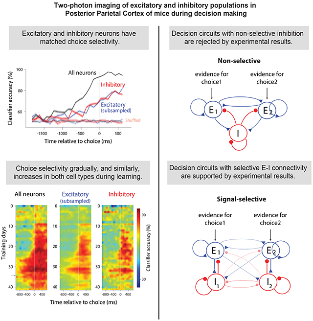
A, Top: Non-selective decision-making model. E1 and E2: pools of excitatory neurons, each favoring a different choice, that excite a single pool of non-selective inhibitory neurons (I). Bottom: Classification accuracy of excitatory (blue) and inhibitory (red) neurons as a function of the relative strength of excitatory-to-inhibitory vs. inhibitory-to-excitatory connections. Arrow in this and subsequent panels: parameter value in line with experimental data. B, Top: Signal-selective model. I1 and I2: pools of inhibitory neurons connected more strongly to E1 and E2, respectively, than to E2 and E1; cross-pool connections are weaker than within-pool connections. Bottom: Decoding accuracy of inhibitory and excitatory neurons match at the biologically plausible regime (arrow). Cross-pool connectivity was 25% smaller than within-pool connectivity. C, Top: SNR-selective model: inhibitory neurons connect more strongly to excitatory neurons with high signal to noise ratios. Bottom: Decoding accuracy of inhibitory and excitatory neurons match near the biologically plausible regime (arrow). All plots reflect 50 excitatory and 50 inhibitory neurons out of a population containing 4000 excitatory/1000 inhibitory neurons.
To test this quantitatively, we modeled a non-selective circuit to evaluate the selectivity of inhibitory neurons (Methods). Classification accuracy depended on the connection strengths between excitatory and inhibitory neurons (horizontal axis on Figure 5A, bottom), as those connection strengths affect overall activity in the network. The most biologically plausible regime is near 0, corresponding to equal strengths for excitatory-to-inhibitory and inhibitory-to-excitatory connections (Thomson and Lamy, 2007; Jouhanneau et al., 2015; Jouhanneau et al., 2018; Znamenskiy et al., 2018) (Figure 5A, bottom, arrow). For this value (and indeed for all other values), inhibitory neurons had lower classification accuracy than excitatory neurons (Figure 5A, bottom; Figure S8, left), inconsistent with our experimental results (Figure 3B,C). Therefore, in the non-selective circuit, although some inhibitory neurons are selective due to random biased inputs from the excitatory pools, classification accuracy of inhibitory neurons will still be lower than excitatory neurons, regardless of the model parameters. This is because even modest amounts of noise in the system are sufficient to overcome any informative randomness in excitatory to inhibitory connections.
Next, we modeled a signal-selective circuit; in which inhibitory neurons were connected preferentially to one excitatory pool (Figure 5B, top). In this circuit architecture, inhibitory and excitatory neurons had matched classification accuracy when the connection strength from excitatory to inhibitory neurons was about the same as the strength from inhibitory to excitatory (Figure 5B, bottom; Figure S8, middle).
Interestingly, a third circuit configuration likewise gave rise to excitatory and inhibitory neurons with matched classification accuracy near the biologically plausible regime (Figure 5C, bottom; Figure S8, right). Here, inhibitory neurons were connected to excitatory neurons with a high signal-to-noise (SNR) ratio (Figure 5C, top).
Our modeling results raise two questions. First, how can the inhibitory population have higher classification accuracy than the excitatory population (Figure 5B,C, bottom; for part of the plot, red is above blue) given that all information about the choice flows through the excitatory neurons. Second, why is the relative strength of the excitatory to inhibitory vs. inhibitory to excitatory connections the critical parameter (Figure 5, bottom; x-axis)? The answers are related. Increasing the strength of the excitatory to inhibitory connections increases the signal in the inhibitory neurons, effectively decreasing the noise added to the inhibitory population (see Methods for details). This decrease in noise leads to improved decoding accuracy of both populations, because they are connected. However, the decrease in the noise added to the inhibitory neurons has a bigger effect on the inhibitory than the excitatory population because the noise directly affects the inhibitory neurons, but only indirectly, through the inhibitory to excitatory connections, affects the excitatory neurons. Thus, in all panels of Figure 5, classification accuracy increases faster for inhibitory neurons than excitatory ones as the excitatory to inhibitory connection strength increases. Interestingly, classification accuracy of both populations was overall higher for the signal-selective and SNR-selective models because the selective targeting in those models mitigates the noise that limits classification accuracy. This advantage was most pronounced for the signal-selective model: the model has significantly higher classification accuracy compared to other models at all values of connectivity strength and noise (Figure S9). This may indicate that the signal-selective network configuration is especially advantageous to accurate decoding in the presence of noise.
Overall, the modeling rules out decision circuits with non-selective inhibition (Figure 5A), and instead demonstrates that excitatory and inhibitory neurons in decision circuits must be selectively connected, either based on the signal preference (Figure 5B) or the informativeness (Figure 5C) of excitatory neurons.
Correlations are stronger between similarly tuned neurons
If choice selectivity in inhibitory neurons emerges because of targeted input from excitatory neurons, one prediction is that correlations will be stronger between excitatory and inhibitory neurons with the same choice selectivity compared to those with the opposite choice selectivity (Cossell et al., 2015; Francis et al., 2018). To test this hypothesis, we compared pairwise noise correlations in the activity of neurons with same vs. opposite choice selectivity (Methods). Indeed, neurons with the same choice selectivity had stronger correlations (Figure 6A), in keeping with previous observations in mouse V1 during passive viewing (Hofer et al., 2011; Ko et al., 2011; Cossell et al., 2015; Znamenskiy et al., 2018), as well as the prefrontal cortex in behaving monkeys (Constantinidis and Goldman-Rakic, 2002).
Figure 6. Pairwise noise correlations are stronger between neurons with the same choice selectivity.

A, Left: Noise correlations (Pearson’s coefficient) for pairs of excitatory-inhibitory neurons with the same (dark green) or opposite (light green) choice selectivity. Middle, right: same as left, but for excitatory-excitatory, and inhibitory-inhibitory pairs, respectively. “Shuffled” denotes quantities were computed using shuffled trial labels. Mean±SEM across days; 0-97 ms before the choice. Same vs. opposite is significant in all cases, except for mouse 3 in EE and II pairs (t-test, p<0.05). B, Example mouse: distribution of noise correlations (Pearson’s correlation coefficients, 0-97 ms before the choice) for excitatory (blue; n=11867) and inhibitory (red; n=1583) neurons. Shaded areas: significance compared to a shuffled control in which trial orders were shuffled for each neuron to remove noise correlations. C, Summary of noise correlation coefficients; mean±SEM across days.
The higher noise correlations among similarly tuned excitatory-inhibitory neuron pairs is also consistent with the observation that in V1, excitatory and inhibitory neurons that belong to the same subnetwork are reciprocally connected (Yoshimura and Callaway, 2005). An alternative explanation, that the neurons with similar tuning share common inputs, is also possible. If that is the case, however, the common input is not exclusively stimulus driven because we observed the same correlation effects in the pre-trial period in which there is no stimulus (Figure S10A).
We next compared the strength of pairwise noise correlations within excitatory and inhibitory populations. Inhibitory pairs had significantly higher noise correlations compared to excitatory pairs (Figure 6B,C: noise correlations; Figure S10C: spontaneous correlations). This was true even when we restricted the analysis to inhibitory and excitatory neurons with the same inferred spiking activity (Figure S10D,E). Finally, similar to previous reports (Hofer et al., 2011; Khan et al., 2018), we found intermediate correlations for pairs consisting of one inhibitory neuron and one excitatory neuron (Figure S10B,C). Our findings align with previous studies in sensory areas reporting stronger correlations among inhibitory neurons (Hofer et al., 2011; Khan et al., 2018). The correlations are likely driven at least in part by local connections, as evidenced by the dense connectivity of interneurons with each other (Galarreta and Hestrin, 1999; Packer and Yuste, 2011; Kwan and Dan, 2012). The difference we observed between excitatory and inhibitory neurons argues that this feature of early sensory circuits is shared by decision-making areas. Further, this clear difference between excitatory and inhibitory neurons, like the difference in inferred spiking (Figure 1G-I) and outcome selectivity (Figure S6C), confirms that we successfully measured two distinct populations. Overall, noise correlation analyses suggest that selective connectivity between excitatory and inhibitory neurons depends on their functional properties.
Noise correlations limit decoding accuracy
Our results thus far demonstrate that neural activity in both excitatory and inhibitory populations reflect an animal’s impending choice (Figure 3B,C), and that there are significant noise correlations among neurons in PPC (Figure 6). However, the analyses so far do not demonstrate how this noise affects the ability to decode neural activity. Examining the effect of noise is essential because correlations affect classifier performance (Panzeri et al., 1999; Averbeck et al., 2006) even when correlations are weak (Averbeck et al., 2006; Moreno-Bote et al., 2014). Fortunately, our dataset with simultaneous activity from hundreds of neurons is especially well-suited to assess noise correlations.
To examine how noise correlations affect classification accuracy, we sorted neurons based on individual choice selectivity, adding them one by one to the population (from highest to lowest choice selectivity defined as ∣AUC-0.5∣). Classification accuracy improved initially as more neurons were included in the decoder, but quickly saturated (Figure 7A, black).
Figure 7. Noise correlations reduce classification accuracy.

A, Classification accuracy for an example session (0-97 ms before the choice) on neural ensembles of increasingly larger size. Mean±SEM (50 cross-validated samples). Gray: classification accuracy for pseudo-populations. Black: real populations. Both cell types were included (“All neurons”). B, Summary for each mouse; points show mean±SEM across days. Values were computed for the largest neuronal ensemble (the max value on the horizontal axis in A).
To assess the effect of noise correlations on classification accuracy, we created “pseudo populations”, in which each neuron in the population was taken from a different trial (Figure 7A gray). This removed noise correlations because those are shared across neurons within a single trial. Higher classification accuracy in pseudo populations compared to real populations indicates the presence of noise that overlaps with signal, limiting information (Panzeri et al., 1999; Averbeck et al., 2006; Averbeck and Lee, 2006; Moreno-Bote et al., 2014). This is what we observed (Figure 7A, gray trace above black trace). In all mice, removing noise correlations resulted in a consistent increase in classification accuracy (Figure 7B; filled vs. open circles), establishing that noise correlations limit population accuracy in PPC.
Selectivity increases in parallel in inhibitory and excitatory populations during learning
Our observations thus far argue that excitatory and inhibitory neurons form selective subnetworks. To assess whether the emergence of these subnetworks is experience-dependent, and if it varies between inhibitory and excitatory populations, we measured neural activity as animals transitioned from novice to expert decision-makers (3 mice; 35-48 sessions; Figure S11). We trained a linear classifier for each training session, and for each moment in the trial.
Classification accuracy of the choice decoder increased consistently as animals became experts in decision-making (Figure 8A, left; Figure 8D, black), leading to a strong correlation between classifier accuracy and mouse performance over training (Figure 8B, left). The choice signal also became more prompt, emerging progressively earlier in the trial as mice became experts. Initially, classification accuracy was high only after the choice (Figure 8A, black arrow). As the animals gained experience, high classification accuracy occurred progressively earlier in the trial, eventually long before the choice (Figure 8A, gray arrow). This resulted in a negative correlation between mouse performance and the onset of super-threshold decoding accuracy (Figure 8C, left; Figure 8E, black).
Figure 8. Learning leads to improved choice decoding, increased fraction of choice-selective neurons, and reduced noise correlations in both populations.

A, Decoder accuracy for each training session, for all neurons (left), subsampled excitatory (middle), and inhibitory neurons (right). White vertical line: choice. Rows: average across cross-validated samples; example mouse. Colorbar applies to both plots. B, Scatter plot of classifier accuracy (0-97 ms before choice) vs. behavioral performance (fraction correct on easy trials) for all training days. r: Pearson correlation coefficient (p<0.001 in all plots); same example mouse as in (A). Correlations for behavior vs. classification accuracy for all neurons, excitatory and inhibitory: 0.55, 0.35, 0.32 in mouse 2; 0.57, 0.63, 0.32 in mouse 3. Correlations for behavior vs. choice-signal onset for all neurons, excitatory and inhibitory: −0.60, −0.34, −0.38, in mouse 2; −0.60, −0.27, −0.28 in mouse 3. All values: p<0.05 C, Same as (B), except showing the onset of choice signal (the first moment in the trial that classifier accuracy was above chance, relative to choice onset) vs. behavioral performance. D, Summary of classification accuracy averaged across early (dim colors) vs. late (dark colors) training days. E, Same as (D), but showing choice signal onset (ms). F, Same as (D), but showing pairwise noise correlation coefficients. EI:excitatory-inhibitory; EE:excitatory-excitatory; II:inhibitory-inhibitory. G, Fraction of choice-selective neurons increases over training; average across early (dim colors) and late (dark colors) training days (0-97 ms before the choice). Early days: first few training days in which the animal’s performance was lower than the 20th percentile of performance across all days. Late days: training days in which performance was above the 80th percentile of performance across all days.
Importantly, the choice signal emerged at the same time in both populations, and its magnitude and timing was matched for the two cell types throughout learning (Figure 8A-C, middle, right; Figure 8D-E, blue, red). This was not due to the presence of more correct trials in later sessions: an improvement in classification accuracy was clear even when the number of correct trials was matched for each session (Figure S13C). These findings indicate that learning induces the simultaneous emergence of choice-specific subpopulations in excitatory and inhibitory cells in PPC.
Notably, the animal’s licking or running behavior could not explain the learning-induced changes in the magnitude of classification accuracy (Figure S12). The center-spout licks preceding left vs. right choices were similar during the course of learning (Figure S12A), and did not differ in early vs. late training days (Figure S12B). The similarity in lick movements for early vs. late sessions contrasts the changes in the classification accuracy for early vs. late sessions (Figure 8). We also assessed running behavior during learning (Figure S12C,D). In some sessions, running distance differed preceding left vs. right choices (Figure S12C). Nonetheless, when we restricted our analysis to days in which running distance was indistinguishable for the two choices (0-97 ms before the choice, t-test, P>0.05), classifiers could still accurately predict the choice (Figure S12D). These observations provide reassurance that population activity does not entirely reflect preparation of licking and running movements, and argue instead that population activity reflects the animal’s stimulus-informed choice.
Finally, we studied how correlations changed over training. Pairwise correlations in neural activity were higher early in training, when mice were novices, compared to late in training, when mice approached expert behavior (Figure 8F, unsaturated colors above saturated colors). This was observed for all combinations of neural pairs (Figure 8F). These findings agree with previous reports suggesting that learning results in reduced noise correlations (Gu et al., 2011; Jeanne et al., 2013; Khan et al., 2018; Ni et al., 2018), enhancing information in neural populations. To test if the learning-induced increase in classification accuracy (Figure 8A,B,D) was entirely a consequence of the reduction in noise correlations (Figure 8F), we studied how classification accuracy of pseudo populations, which lack noise correlations, changed with training. Interestingly, a significant increase in the classification accuracy of pseudo populations was present (Figure S13A,B). Therefore, the reduction in noise correlations cannot alone account for the improved classification accuracy during learning, suggesting that increased choice selectivity of individual neurons also contributes. Indeed, the fraction of choice-selective neurons increased threefold during training, in both excitatory and inhibitory neurons (Figure 8G).
Discussion
Despite a wealth of studies assessing selectivity of inhibitory neurons for sensory features, little is known about the selectivity of inhibitory neurons in decision-making. This is a critical gap, and has left untested key features of decision-making models relying on inhibitory neurons. To close this gap, we simultaneously measured excitatory and inhibitory populations during perceptual decisions about multisensory stimuli.
We found that excitatory and inhibitory neurons predict the animal’s impending choice with equal fidelity (Figure 2,3). This result, along with our modeling (Figure 5), constrains circuit models of decision-making, ruling out models in which inhibitory neurons receive completely nonspecific input from excitatory populations (Figure 5A). Instead, our findings suggest that specific functional subnetworks exist within inhibitory populations, just like excitatory populations (Figure 5B). This implies targeted connectivity between excitatory and inhibitory neurons (Yoshimura and Callaway, 2005; Znamenskiy et al., 2018), and supports circuit architectures with functionally specific, reciprocally connected subnetworks.
A documented advantage of signal-selective architectures is that they can offer improved stability (Znamenskiy et al., 2018) and robustness to perturbations (Lim and Goldman, 2013). However, in our circuit, selectivity did not improve stability but instead improved performance: classification accuracy for the signal selective model was the highest of the three we tested (Figure 5B, bottom row, Figure S9). These observations raise the possibility that among possible circuit architectures that could have been leveraged by the brain to support decision-making, the highest-performing one was chosen.
The equal selectivity for choice that we observed in excitatory and inhibitory populations is perhaps, at first, surprising, given the broad stimulus tuning curves observed in most V1 inhibitory neurons (Sohya et al., 2007; Niell and Stryker, 2008; Kerlin et al., 2010; Bock et al., 2011; Hofer et al., 2011; Znamenskiy et al., 2018) (but see Runyan et al., 2010) and the dense connectivity for inhibitory neurons (Hofer et al., 2011; Packer and Yuste, 2011; Znamenskiy et al., 2018). Two differences between our study and previous ones may explain why we saw equal selectivity in excitatory and inhibitory populations.
First, we measured neural activity in PPC where the proportion of interneuron subtypes differs from V1: V1 is enriched for PV interneurons relative to SOM and VIP neurons, whereas the opposite is true in association areas (Kim et al., 2017; Wang and Yang, 2018). Moreover, interneuron subtypes vary in their specificity of connections (Pfeffer et al., 2013); for instance, PV interneurons have broader tuning than SOM and VIP cells (Wang et al., 2004; Ma et al., 2010). Therefore, the strong selectivity we found in all GABAergic interneurons in PPC may not contradict the broad selectivity observed in studies largely performed on PV interneurons in V1. Future studies that measure the selectivity of distinct interneuron populations during decision-making in V1 vs. PPC will be helpful. Here, we measured all GABAergic interneurons instead of individual interneuron subtypes because of the technical challenge in reliably identifying more than two cell types in a single mouse, and because of the importance of simultaneously measuring the activity of excitatory and inhibitory neurons within the same subject. Had we lacked within-mouse measurements, our ability to compare excitatory vs. inhibitory neurons would have been compromised by mouse-to-mouse variability (note matched selectivity of excitatory and inhibitory neurons within mice in Figure 3C despite overall variability across mice).
Second, analyzing neural activity in the context of decision-making naturally led us to make different comparisons than those carried out previously. For example, we measured selectivity for a binary choice, while sensory tuning curves are measured in response to continuously varying stimuli (e.g., orientation). Further, we measured activity in response to abstract stimuli, the meaning of which was learned gradually by the animal. This may recruit circuits that differ from those supporting sensory processing in passively viewing mice. Finally, we used stochastically fluctuating multisensory stimuli, which have not been evaluated in mouse V1.
Future studies that examine the tuning of V1 neurons to the sensory stimulus used here will determine if V1 inhibitory neurons will be as sharply tuned as excitatory neurons to the stimulus. This is a possibility: the tuning strength of interneurons can vary substantially for different stimulus features. For instance, PV neurons in V1 have particularly poor tuning to orientation, but their temporal-frequency tuning is considerably stronger (Znamenskiy et al., 2018).
We not only studied expert animals, but also evaluated how acquiring expertise modulates activity. We observed that learning increased the number of choice-selective neurons and decreased noise correlations, indicating plasticity and reorganization of connections. Population responses preceding the two choices thus became progressively more distinct with training. Importantly, these changes occur in parallel in excitatory and inhibitory cells. Our findings are partially in agreement with those in V1, in which learning improves tuning to sensory stimuli in excitatory (Schoups et al., 2001; Poort et al., 2015; Khan et al., 2018) and some inhibitory (Khan et al., 2018) neurons. However, V1 excitatory neurons have stronger tuning to sensory stimuli early in training (Khan et al., 2018); in contrast, in our study, the magnitude of choice selectivity in PPC was the same for both cell types throughout training (Figure 8). Primate studies have likewise observed that perceptual learning changes the selectivity of neurons (Freedman and Assad, 2006; Law and Gold, 2008; Viswanathan and Nieder, 2015) and reduces noise correlations (Gu et al., 2011; Ni et al., 2018).
Finally, we demonstrated that learning-induced changes in selectivity were closely associated with changes in animal performance, in keeping with primate studies of decision-making (Law and Gold, 2008). This, together with our finding that changes in population activity do not purely reflect movements (Figure S12), corroborates the suggested role for PPC in mapping sensation to action (Law and Gold, 2008; Raposo et al., 2014; Pho et al., 2018). Future experiments using causal manipulations will reveal whether the increased choice selectivity we observed in PPC originates there or is inherited from elsewhere in the brain.
By measuring cell-type-specific activity in parietal cortex during decision-making, we observed that excitatory and inhibitory populations are equally choice-selective, and that these ensembles emerge in parallel, as mice become skilled decision-makers. These results argue against models with non-specific connectivity between excitatory and inhibitory neurons, at least in decision circuits. Future modeling efforts can incorporate subnetworks and evaluate their impact on key model outputs, such as reaction time distributions and firing rates. Such studies will shed light on how microcircuits of inhibitory and excitatory neurons vary across areas in their selectivity and specificity of connections, and will reveal the circuit architectures that allow for equally selective inhibitory and excitatory neurons.
STAR Methods
Lead contact and materials availability
Lead contact for additional inquiry: churchland@cshl.edu. This study did not generate new unique reagents.
Experimental model and subject details
Gad2-IRES-CRE (Taniguchi et al., 2011) mice were crossed with Rosa-CAG-LSL-tdTomato-WPRE (aka Ai14; Madisen et al., 2010) to create mice in which all GABAergic inhibitory neurons were labeled. Adult mice (~2-month old; female and male) were used in the experiments.
Method Details
Surgical procedure
Meloxicam (analgesic), dexamethasone (anti-inflammatory) and Baytril (enrofloxacin; antibiotic) were injected 30min before surgery. Using a biopsy punch, a circular craniotomy (diameter: 3mm) was made over the left PPC (stereotaxic coordinates: 2 mm posterior, 1.7 mm lateral of bregma (Harvey et al., 2012) under isoflurane (~5%) anesthesia. Pipettes (10-20 um in diameter, cut at an angle to provide a beveled tip) were front-filled with AAV9-Synapsin-GCaMP6f (U Penn, Vector Core Facility) diluted 2X in PBS (Phosphae-buffered saline). The pipette was slowly advanced into the brain (Narishige MO-8 hydraulic micro-manipulator) to make ~3 injections of 50nL, slowly over an interval of ~5-10 min, by applying air pressure using a syringe. Injections were made near the center of craniotomy at a depth of 250-350 μm below the dura. A glass plug consisting of a 5mm coverslip attached to a 3mm coverslip (using IR-curable optical bond, Norland) was used to cover the craniotomy window. Vetbond, followed by metabond, was used to seal the window. All surgical and behavioral procedures conformed to the guidelines established by the National Institutes of Health and were approved by the Institutional Animal Care and Use Committee of Cold Spring Harbor Laboratory.
Imaging
We used a 2-photon Moveable Objective Microscope with resonant scanning at approximately 30 frames per second (Sutter Instruments, San Francisco, CA). A 16X, 0.8 NA Nikon objective lens was used to focus light on fields of view of size 512×512 pixels (~575 μm × ~575 μm). A Ti:sapphire laser (Coherent) delivered excitation light at 930nm (average power: 20-70 mW). Red (ET670/50m) and green (ET 525/50m) filters (Chroma Technologies) were used to collect red and green emission light. The microscope was controlled by Mscan (Sutter). In mice in which chronic imaging was performed during learning, the same plane was identified on consecutive days using both coarse alignment, based on superficial blood vessels, as well as fine alignment, using reference images of the red channel (tdTomato expression channel) at multiple magnification levels. For each trial, imaging was started 500ms before the trial-initiation tone, and continued 500ms after reward or time-out. We aimed to image in the center of the window for all mice, but in one animal (Mouse 4), some tissue regrowth obscured the signal in this region and so imaging was performed slightly further back.
Decision-making behavior
Mice were gradually water restricted over the course of a week, and were weighed daily. Mice harvested at least 1 mL of water per behavioral/imaging session, and completed 100-500 trials per session. After approximately one week of habituation to the behavioral setup, 15-30 training days were required to achieve 75% correct choice. Animal training took place in a sound isolation chamber. The stimulus in all trials was multisensory, consisting of a series of simultaneous auditory clicks and visual flashes, occurring with Poisson statistics (Brunton et al., 2013; Odoemene et al., 2017). Multisensory stimuli were selected because they increased the learning rate of the mice, a critical consideration since GCaMP6f expression can be unreliable over a long period of time. Stimulus duration was 1000 ms. Each pulse was 5 ms; minimum interval between pulses was 32 ms, and maximum interval was 250 ms. The pulse rate ranged from 5 to 27 Hz. The category boundary for marking high-rate and low-rate stimuli was 16 Hz, at which animals were rewarded randomly on either side. The highest stimulus rates used here are known to elicit reliable, steady state flicker responses in retinal ERG in mice (Krishna et al., 2002; Tanimoto et al., 2015).
Mice were on top of a cylindrical wheel and a rotary encoder was used to measure their running speed. Trials started with a 50 ms initiation tone (Figure S1A). Mice had 5 sec to initiate a trial by licking the center waterspout (Marbach and Zador, 2017), after which the multisensory stimulus was played for 1 second. If mice again licked the center waterspout, they received 0.5 μL water on the center spout, and a 50ms go cue was immediately played. Animals had to report a choice by licking to the left or right waterspout within 2 sec. Mice were required to confirm their choice by licking the same waterspout one more time within 300 ms after the initial lick (Marbach and Zador, 2017). The “confirmation lick” helped dissociate the choice time (i.e. the time of first lick to the side waterspout), from the reward time (i.e. the time of second lick to the side waterspout); it also helped with reducing impulsive choices. If the choice was correct, mice received 2-4 μL water on the corresponding waterspout. An incorrect choice was punished with a 2 sec time-out. The experimenter-imposed inter-trial intervals (ITIs) were drawn from a truncated exponential distribution, with minimum, maximum, and lambda equal to 1 sec, 5 sec, and 0.3 sec, respectively. However, the actual ITIs could be much longer depending on when the animal initiates the next trial. Bcontrol (Raposo et al., 2014) with a Matlab interface was used to deliver trial events (stimulus, reward, etc) and collect data.
Logistic regression model of behavior
A modified version of a logistic regression model in (Busse et al., 2011) was used to assess the extent to which the animal’s choice depends on the strength of sensory evidence (how far the stimulus rate is from the category boundary at 16Hz), the previous choice outcome (success or failure) and ITI, (the time interval between the previous choice and the current stimulus onset) (Figure S1B). The model has the form
| eq.1 |
where p is the probability of choosing left. Stimulus strength (R) was divided into 6 bins (R1 to R6). Previous success (S) was divided into 2 bins (S1 to S2), with S1 referring to success after a long ITI (> 7sec) and S2 to success after a short ITI (< 7sec). Previous failure (F) was divided into 2 bins (F1 to F2), with F1 referring to failure after a long ITI and F2 to failure after a short ITI. For example, if a trial had stimulus strength 3 Hz, and was preceded by a success choice with ITI 5 sec, then R2 and S1 would be set to 1 and all other R, S and F parameters to 0 (Figure S1B).
For each session the scalar coefficients β0, βr1 to βr6, βs1, βs2, βf1, and βf2 were fit using Matlab glmfit.m. Figure S1B left shows βr1 to βr6. Figure S1B middle shows βs1 and βs2, and Figure S1B right shows βf1 and βf2.
ROI (region of interest) extraction and deconvolution
The recorded movies from all trials were concatenated and corrected for motion artifacts by cross-correlation using Discrete Fourier Transform (DFT) registration (Guizar-Sicairos et al., 2008). Subsequently, active ROIs (sources) were extracted using the Constrained Nonnegative Matrix Factorization (CNMF) algorithm (Pnevmatikakis et al., 2016) as implemented in the CaImAn package (Giovannucci et al., 2019) in MATLAB. The traces of the identified neurons were ΔF/F normalized and then deconvolved by adapting the FOOPSI deconvolution algorithm (Vogelstein et al., 2010; Pnevmatikakis et al., 2016) to a multi-trial setup. This was necessary because simply concatenating individual trials would lead to discontinuities in the traces, which could distort estimates of the time constants. Each value of Foopsi deconvolution represents spiking activity at each frame for a given neuron. We have referred to the deconvolved values as "inferred spiking activity" throughout the paper. The deconvolved values do not represent absolute firing rates, so they cannot be compared across neurons. However, for a particular neuron, higher inferred spiking activity means higher firing rate. We elected to base our analyses on inferred spiking activity rather than fluorescence activity because peak amplitudes and time constants of the fluorescence responses vary across neurons, affecting subsequent analyses (Machado et al., 2015; Helmchen and Tank, 2019).
We adapted the FOOPSI for multi-trial setup as follows. For each component, the activity trace over all the trials was used to determine the time constants of the calcium indicator dynamics as in (Pnevmatikakis et al., 2016). Then the neural activity during each trial was deconvolved separately using the estimated time constant and a zero baseline (since the traces were ΔF/F normalized). A difference of exponentials was used to simulate the rise and decay of the indicator.
Neuropil Contamination removal
The CNMF algorithm demixes the activity of overlapping neurons. It takes into account background neuropil activity by modeling it as a low rank spatiotemporal matrix (Pnevmatikakis et al., 2016). In this study a rank two matrix was used to capture the neuropil activity. To evaluate its efficacy, we compared the traces obtained from CNMF to the traces from a “manual” method similar to (Chen et al., 2013) (Figure S14): the set of spatial footprints (shapes) extracted from CNMF were binarized by thresholding each component at 20% of its maximum. The binary masks were then used to average the raw data and obtain an activity trace that also included neuropil effects. To estimate the background signal, an annulus around the binary mask was constructed with minimum distance 3 pixels from the binary mask and width 7 pixels (Figure S14A). The average of the raw data over the annulus defined the background trace, which was subtracted from the activity trace. The resulting trace was then compared with the CNMF estimated temporal trace for this activity. The comparison showed a very high degree of similarity between the two traces (Figure S14; example component; r=0.96), with the differences between the components being attributed to noise and not neuropil related events. Note that this “manual” approach is only applicable in the case when the annulus does not overlap with any other detected sources. These results demonstrate the ability of the CNMF framework to properly capture neuropil contamination and remove it from the calcium traces.
ROI inclusion criteria
We excluded poor-quality ROIs identified by the CNMF algorithm based on a combination of criteria: 1) size of the spatial component, 2) decay time constant, 3) correlation of the spatial component with the raw ROI image built by averaging spiking frames, 4) correlation of the temporal component with the raw activity trace, and 5) the probability of fluorescence traces maintaining values above an estimated signal-to-noise level for the expected duration of a calcium transient(Giovannucci et al., 2018) (GCaMP6f, frame rate: 30Hz). A final manual inspection was performed on the selected ROIs to validate their shape and trace quality.
Identification of inhibitory neurons
We used a two-step method to identify inhibitory neurons. First, we corrected for bleed-through from green to red channel by considering the following regression model,
| eq.2 |
where, ri(t) and gi(t) are vectors, indicating pixel intensity in red and green channel, respectively, with each component of the vector corresponding to one pixel in the ROI, i labels ROI (presumably each ROI is a neuron), βi is the offset, 1p is a vector whose components are all 1, and s is the parameter that tells us how much of the green channel bleeds through to the red one.
It is the parameter s that we are interested in. To find s, we define a cost function, C,
| eq.3 |
and minimize it with respect to s and all the βi. The value of s at the minimum reflects the fraction of bleed-through from the green to the red channel. That value, denoted s*, is then used to compute the bleedthrough-corrected image of the red-channel, denoted I via the expression
| eq.4 |
where R and G are the time-averaged images of the red and green channels, respectively.
Once the bleedthrough-corrected image, I, was computed, we used it to identify inhibitory neurons using two measures,
1) A measure of local contrast, by computing, on the red channel (I, eq. 4), the average pixel intensity inside each ROI mask relative to its immediate surrounding mask (width=3 pixels). Given the distribution of contrast levels, we used two threshold levels, TE and TI, defined, respectively, as the 80th and 90th percentiles of the local contrast measures of all ROIs. ROIs whose contrast measure fell above TI were identified as inhibitory neurons. ROIs whose contrast measure fell below TE were identified as excitatory neurons, and ROIs with the contrast measure in between TE and TI were not classified as either group (“unsure” class).
2) In addition to a measure of local contrast, we computed for each ROI the correlation between the spatial component (ROI image on the green channel) and the corresponding area on the red channel. High correlation values indicate that the ROI on the green channel has a high signal on the red channel too; hence the ROI is an inhibitory neuron. We used this correlation measure to further refine the neuron classes computed from the local contrast measure (i.e. measure 1 above). ROIs that were identified as inhibitory based on their local contrast (measure 1) but had low red-green channel correlation (measure 2), were reset as “unsure” neurons. Similarly, ROIs that were classified as excitatory (based on their local contrast) but had high red-green channel correlation were reclassified as unsure. Unsure ROIs were included in the analysis of all-neuron populations (Figure 3A left); but were excluded from the analysis of excitatory only or inhibitory only populations (Figure 3A middle, right). Finally, we manually inspected the ROIs identified as inhibitory to confirm their validity. This method resulted in 11% inhibitory neurons, which is within the range of previous studies (10-20%: Rudy et al., 2011); (15%: Beaulieu, 1993); (16%: Gabbott et al., 1997); (<5%: de Lima and Voigt, 1997); (10-25%: de Lima et al., 2009).
ROC analysis
The area under the ROC curve (AUC) was used to measure the choice preference of single neurons. Choice selectivity was defined as the absolute deviation of AUC from chance level: choice selectivity = 2*∣AUC-0.5∣. To identify significantly choice-selective neurons, for each neuron we performed ROC on shuffled trial labels (i.e. left and right choices were randomly assigned to each trial). This procedure was repeated 50 times to create a distribution of shuffled AUC values for each neuron (Figure S3A, “shuffled”). A neuron’s choice selectivity was considered to be significant if the probability of the actual AUC (Figure S3A, “real”) being drawn from the shuffled AUC distribution was less than 0.05. Time points from 0–97 ms before the decision were used to compute the fraction of choice-selective neurons (Figure 2B; Figure 8G).
Decoding population activity
A linear SVM (Python sklearn package) was trained on each bin of the population activity in each session (non-overlapping 97ms time bins). To break any dependencies on the sequence of trials, we shuffled the order of trials for the entire population. To avoid bias in favor of one choice over the other, we matched the number of left- and right-choice trials used for classifier training. L2 regularization was used to avoid over-fitting. 10-fold cross validation was performed by leaving out a random 10% subset of trials to test the classifier performance, and using the remaining trials for training the classifier. This procedure was repeated 50 times. A range of regularization values was tested, and the one that gave the smallest error on the validation dataset was chosen as the optimal regularization parameter. Classifier accuracy was computed as the percentage of testing trials in which the animal’s choice was accurately predicted by the classifier, and summarized as the average across the 50 repetitions of trial subsampling. A minimum of 10 correct trials per choice was required in order to run the SVM on a session. Inferred spiking activity of each neuron was z-scored before running the SVM.
When comparing classification accuracy for excitatory vs. inhibitory neurons, the excitatory population was randomly sub-sampled to match the population size of inhibitory neurons to enable a fair comparison (Figure 3, blue vs. red). To compare the distribution of weights in the all-neuron classifier (Figure 3 black), the weight vector for each session was normalized to unity length (Figure 3D-F).
When decoding the stimulus category (Figure S6B), we used stimulus-aligned trials, and avoided any contamination by the choice signal by sub-selecting equal number of left and right choice trials for each stimulus category. When decoding trial outcome (Figure S6C), we used outcome-aligned trials, and avoided contamination by the choice or stimulus signal by subselecting equal number of trials from left and right choice trials for each trial outcome.
Stability
To test the stability of the population code, decoders were trained and tested at different time bins (Kimmel et al., 2016) (Figure 4). To avoid the potential effects of auto-correlation, we performed cross validation not only across time bins, but also across trials. In other words, even though the procedure was cross validated by testing the classifier at a time different from the training time, we added another level of cross-validation by testing on a subset of trials that were not used for training. This strict method allowed our measure of stability duration to be free of auto-correlation effects.
As an alternative measure of stability, the angle between pairs of classifiers that were trained at different moments in the trial was computed (Figure S7C). Small angles indicate alignment, hence stability, of the classifiers. Large angles indicate misalignment, i.e. instability of the classifiers.
Noise correlations
To estimate noise correlations, the order of trials was shuffled for each neuron independently. Shuffling was done within the trials of each choice, hence retaining the choice signal, while de-correlating the population activity to remove noise correlations. Then we classified population activity in advance of left vs. right choice (at time bin 0–97 ms before the choice) using the de-correlated population activity. This procedure was performed on neural ensembles of increasingly larger size, with the most selective neurons (the ones with the largest value of ∣AUC-0.5∣) added first (Figure 7A). To summarize how noise correlations affected classification accuracy in the population (Figure 7B), we computed, for the largest neural ensemble (Figure 7A, max value on the horizontal axis), the change in classifier accuracy in the de-correlated data (“pseudo populations”) vs. the original data. This analysis was only performed for the entire population; the small number of inhibitory neurons in each session prevented a meaningful comparison of classification accuracy on real vs. pseudo populations.
To measure pairwise noise correlations, we subtracted the trial-averaged response to a particular choice from the response of single trials of that choice. This allowed removing the effect of choice on neural responses. The remaining variability in trial-by-trial responses can be attributed to noise correlations, measured as the Pearson correlation coefficient for neuron pairs. We also measured noise correlations using the spontaneous activity defined as the neural responses in 0-97 ms preceding the trial initiation tone (Figure S10A,C). We computed the pairwise correlation coefficient (Pearson) for a given neuron with each other neuron within an ensemble (e.g., excitatory neurons). The resulting coefficients were then averaged to generate a single correlation value for that neuron. This was repeated for all neurons within the ensemble (Figure 6).
To compute pairwise correlations on excitatory and inhibitory neurons with the same inferred spiking activity (Figure S10D,E), we computed the median inferred spiking activity across trials for individual excitatory and inhibitory neurons in a session. The medians were then divided into 50 bins. The firing-rate bin that included the maximum number of inhibitory neurons was identified (“max bin”); inhibitory and excitatory neurons whose firing rate was within this “max bin” were used for the analysis. The firing rates were matched for these neurons because their median firing rate was within the same small bin of firing rates. Pairwise correlations were then computed as above.
Learning analysis
In 3 of the mice, the same field of view was imaged each session during learning. This was achieved in two ways. First, the vasculature allowed a coarse alignment of the imaging location from day to day. Second, the image from the red channel was used for a finer alignment. Overall, most neurons were stably present across sessions (Figure S11). This suggests that we likely measured activity from a very similar population each day. Importantly, however, our conclusions do not rely on this assumption: our measures and findings focus on learning-related changes in the PPC population overall, as opposed to tracking changes in single neurons. To assess how population activity changed over learning, we evaluated classification accuracy each day, training a new decoder for each session. This approach allowed us to compute the best decoding accuracy for each session.
“Early days” (Figure 8; Figures S12,S13) included the initial training days in which the animal’s performance, defined as the fraction of correct choices on easy trials, was lower than the 20th percentile of performance across all days. “Late days” (Figure 8; Figures S12,S13) included the last training days in which the animal’s behavioral performance was above the 80th percentile of performance across all days.
To measure the timing of decision-related activity (Figure 8C,E), we identified all sessions in which classifier accuracy was significantly different than the shuffle (t-test, p<0.05) over a window of significance that was at least 500 ms long. We defined the “choice signal onset” (Figure 8C,E) as the trial time corresponding to the first moment of that window. Sessions in which the 500 ms window of significance was present are included in Figure 8C. The number of points (and hence the relationship between session number and color in Figure 8C) differs slightly across the three groups. This is because on some sessions, the window of significance was present in one group but not another. For example, in a session the population including all neurons might have a 500 ms window of significance, hence it will contribute a point to Figure 7C left, while the population with only inhibitory neurons might be only transiently significant for <500ms, hence it will be absent from Figure 8C right.
Modeling decision circuits
We considered a linearized rate network of the form
where E and I refer to the excitatory and inhibitory populations, respectively, νE and νI are vectors of firing rates (νE = νE1, νE2, …, and similarly for νI), WEE, WEI, WIE and WII are the connectivity matrices (WEI indicates connection from inhibitory to excitatory neuron), hs is the input, with s either 1 or 2 (corresponding to left and right licks), and ξ is trial to trial noise, taken to be zero mean and Gaussian, with covariance matrices
For the input we’ll assume that about half the elements of hs are h0 for the rightward choice and −h0 for the leftward choice, and the rest are −h0 for the rightward choice and h0 for the leftward choice. We used h0 = 0.1. The noise covariance is diagonal but non-identity, with diagonal elements distributed as
The goal is to determine the value of s (that is, determine whether h1 or h2 was present) given the activity of a subset of the neurons from either the excitatory or inhibitory populations. We’ll work in steady state, for which
Solving for νE and νI yields
where
and I is the identity matrix. We are interested in the decoding accuracy of a sub-population of neurons. For that we’ll use a matrix Dn that picks out n components of whatever it’s operating on. So, for instance, Dn · νE is an n-dimensional vector with components equal to n of the components of νE.
For a linear and Gaussian model such as ours, in which the covariance is independent of s, we need two quantities to compute the performance of an optimal decoder: the difference in the means of the subsampled populations when h1 vs. h2 are present, and covariance matrix of the subsampled populations. The difference in means are given by
where Δh is the difference between the two inputs,
The covariances are given by
where T denotes transpose. Combining the mean and covariance gives us the signal to noise ratio,
The performance of an optimal decoder is then given by
where Φ is the cumulative normal function. All of our analysis is based on this expression. Differences in fraction correct depend only on differences in the connectivity matrices, which we describe next.
Connectivity matrices
We consider three connectivity structures: completely non-selective, signal-selective, and signal-to-noise selective (corresponding to Figures 5A, 5B and 5C, respectively). In all cases the connectivity is sparse (the connection probability between any two neurons is 0.1). What differs is the connection strength when neurons are connected. We describe below how the connection strength is chosen for our three connectivity structures.
Non-selective.
The connectivity matrices have the especially simple form
where α, β ∈ {E, I}, N(≡ NE + NI) is the total number of neurons, and wαβ are parameters.
Signal-selective.
We divide the neurons into two sets of excitatory and inhibitory sub-populations, as in Figure 5B. The connection strengths are still given by the above expression, but now α and β acquire subscripts that specify which population they are in: α, β ∈ {E1, E2, I1, I2}, with E1 and I1 referring to population 1 and E2 and I2 to population 2. The within-population connection strengths are the same as for the non-selective population (wαiβi = wαβ, i = 1, 2), but the across-population connection strengths are smaller by a factor of ρ,
for i = 1 and j = 2 or vice-versa. The value of ρ determines how selective the sub-populations are: ρ = 0 corresponds to completely selective sub-populations while ρ = 1 corresponds to the completely non-selective case.
SNR- selective.
We choose the connectivity as in the non-selective case, and then change synaptic strength so that the inhibitory neurons receive stronger connections from the excitatory neurons with high signal to noise ratios. To do that, we first rank excitatory units in order of ascending signal to noise ratio (by using D1 in the expression for (S/N)E in the previous section). We then make the substitution
where rj is the rank of excitatory j in the order of ascending signal to noise ratio and, recall, NE is the number of excitatory neurons. This downweights projections from low signal to noise ratio excitatory neurons and upweights connections from high signal to noise ratio neurons. Finally, all elements are scaled to ensure that the average connection strength from the excitatory to the inhibitory network is the same as before the substitution.
Simulation details
Noise level (σ) = 1.25
Breadth of noise level distribution (δ) = 0.75
Excitatory → excitatory coupling (wEE) = 0.25
Inhibitory → inhibitory coupling (wII) = −2
Excitatory → inhibitory coupling (reference) (wIE(0)) = 0.87
Inhibitory → excitatory coupling (reference) (wEI(0)) = −0.87
Connection probability (c) = 0.1
Number of excitatory neurons (NE) = 4000
Number of inhibitory neurons (NI) = 1000
Number of readout neurons (n) = 50
Input strength (h0) = 0.1
Selectivity index (ρ) = 0.75
The simulation parameters are indicated above. In addition, there are a number of relevant details, the most important of which is related to the input, hs. As mentioned in the previous section, about half the elements of hs are h0 for the rightward choice and −h0 for the leftward choice, and the rest are h0 for the leftward choice −h0 for the rightward choice. This is strictly true for the completely non-selective and signal to noise selective connectivity; for the signal selective connectivity, we use hs,i = h0 for the rightward choice and −h0 for the leftward choice when excitatory neuron i is in population 1, and hs,i = h0 for the leftward choice and −h0 for the rightward choice when excitatory neuron i is in population 2. In either case, however, this introduces a stochastic element: for the completely non-selective and signal to noise selective connectivities, there is randomness in both the input and the circuit; for the signal selective connectivity, there is randomness in the circuit. In the former case, we can eliminate the randomness in the connectivity by averaging over the input, as follows.
Because the components of Δh are independent, we have
where δij is the Kronecker delta (δij = 1 if i = j and zero otherwise). Because Δhs,i is either +h0 or −h0, we have
where I is the identity matrix. Thus, when we average the signal to noise ratios over Δh, the expressions simplify slightly,
To avoid having to numerically average over input, we used these expressions when computing decoding accuracy for the completely non-selective and signal to noise selective connectivity. That left us with some randomness associated with the networks (as connectivity is chosen randomly), but that turned out to produce only small fluctuations, so each data point in Figures 5A and 5C was from a single network. For the signal selective connectivity (Figure 5B), the network realization turned out to matter, so we averaged over 25 networks, and for each of them we did a further averaging over 100 random picks of the 50 neurons from which we decoded.
In Figure 5, the x-axis is the ratio of the average connection strength from excitatory to inhibitory neurons to the average connection strength from inhibitory to excitatory neurons. This was chosen because it turned out to be the connectivity parameter with the largest effect on decoding accuracy. That in turn is because it turns out to be equivalent to the input noise to the inhibitory population. To see why, make the substitution
By letting νI → γνI, we see that this is formally equivalent to letting ξI → γ−1ξI, which in turn corresponds to letting ΣII → γ−2ΣII. Thus the x-axis in Figure 5 can be thought of as the axis of decreasing input noise to the inhibitory neurons.
We produced a range of values for γ by changing the coupling strengths between excitatory and inhibitory populations, while keeping their product constant at a reference value
Immunofluorescence staining for TdTomato and GABA
To determine the fraction of inhibitory neurons that were labeled in our experiments, we performed double Immunofluorescence (IF) staining using antibodies against tdTomato (anti-RFP(tdTomato) Rockland 600-401-379) and GABA (anti-GAD67(GABA) MAB5406, EMD Millipore). Also, we used DAPI to stain the nuclei (Figure S15; GABA: green; tdTomato: red; DAPI: blue). 5 coronal sections which included the area PPC (Allen Brain Atlas) were used to quantify the fraction of overlap between GABA and tdTomato. We found GABA and tdTomato highly colocalized (Figure S15B-D; red and green are co-expressed in the vast majority of cells): 98.2 % of tdTomato neurons expressed GABA, and all of the GABAergic neurons expressed tdTomato. These results indicate a very high level of selectivity and specificity for the labeling of inhibitory neurons in GAD-Cre;Ai14 mice, confirming original reports for these transgenic lines (Taniguchi et al., 2011).
Quantification and statistical analysis
Our simultaneous imaging and decision-making dataset includes 135 sessions from 4 mice (45, 48, 7, and 35 sessions per mouse). Median number of trials per session is 213, 253, 264, and 222, for each mouse. On average, 480 neurons were imaged per session, out of which ~40 neurons were inhibitory and ~330 were excitatory. Approximately 100 neurons per session were not classified as either excitatory or inhibitory since they did not meet our strict cell-type classification criteria (see below). In 3 of the mice, the same group of neurons was imaged throughout learning (35-48 training days).
All analyses were performed on inferred spiking activity. Traces were down-sampled, so each bin was the non-overlapping moving average of 3 frames (97.1 ms, which we refer to as 97 ms). Inferred spiking activity for each neuron was normalized so the max spiking activity for each neuron equaled 1. The trace of each trial was aligned to the time of the choice (i.e. the time of the 1st lick to either of the side waterspouts after the go tone). Two-tailed t-test was performed for testing statistical significance. Summary figures including all mice were performed on the time bin preceding the choice, i.e. 0-97 ms before choice onset. All reported correlations are Pearson’s coefficients. Analyses were performed in Python and Matlab.
Data and code availability
All the data used in the paper are publicly available on CSHL repository: http://repository.cshl.edu/36980/. Further, all the data is converted into the NWB format (Neurodata Without Boarders (Teeters et al., 2015; Ruebel et al., 2019), and is available on CSHL repository: https://dx.doi.org/10.14224/1.37693
Code for data processing and analysis is publicly available on github: https://github.com/farznaj/imaging_decisionMaking_exc_inh
Code for converting data to NWB format is also available on github:https://github.com/vathes/najafi-2018-nwb
Supplementary Material
Highlights:
Excitatory and inhibitory neurons are equally selective during decision-making
Selectivity of the two cell types increases in parallel during learning
Models and experiments reject decision circuits with non-selective inhibition.
Selective subnetworks of neurons emerge during learning to support decision-making
Acknowledgements
We thank Hien Nguyen for mouse training, Matt Kaufman, Kachi Odoemene, Fred Marbach for technical expertise and thoughtful conversations. We thank Andrea Giovannucci for help with ROI inclusion criteria #5. We thank Ashley Juavinett, Simon Musall, and Sashank Pisupati for helpful discussions and feedback on early versions of the manuscript. We thank Thinh Nguyen, Dimitri Yatsenko and Edgar Walker for help with data conversion into the NWB format. The work was supported by the Simons Collaboration on the Global Brain (AKC), the Army Research Office (ARO) under contract W911NF-16-1-0368 (AKC and PEL), the Klingenstein-Simons Foundation (AKC), the Pew Charitable Trust (AKC) and the Gatsby Charitable Foundation (PEL).
Footnotes
Publisher's Disclaimer: This is a PDF file of an unedited manuscript that has been accepted for publication. As a service to our customers we are providing this early version of the manuscript. The manuscript will undergo copyediting, typesetting, and review of the resulting proof before it is published in its final form. Please note that during the production process errors may be discovered which could affect the content, and all legal disclaimers that apply to the journal pertain.
Declaration of Interests
There are no competing interests.
References
- Akrami A, Kopec CD, Diamond ME, Brody CD (2018) Posterior parietal cortex represents sensory history and mediates its effects on behaviour. Nature 554:368–372. [DOI] [PubMed] [Google Scholar]
- Allen WE, Kauvar IV, Chen MZ, Richman EB, Yang SJ, Chan K, Gradinaru V, Deverman BE, Luo L, Deisseroth K (2017) Global Representations of Goal-Directed Behavior in Distinct Cell Types of Mouse Neocortex. Neuron 94:891–907 e896. [DOI] [PMC free article] [PubMed] [Google Scholar]
- Atallah BV, Bruns W, Carandini M, Scanziani M (2012) Parvalbumin-expressing interneurons linearly transform cortical responses to visual stimuli. Neuron 73:159–170. [DOI] [PMC free article] [PubMed] [Google Scholar]
- Averbeck BB, Lee D (2006) Effects of noise correlations on information encoding and decoding. J Neurophysiol 95:3633–3644. [DOI] [PubMed] [Google Scholar]
- Averbeck BB, Latham PE, Pouget A (2006) Neural correlations, population coding and computation. Nat Rev Neurosci 7:358–366. [DOI] [PubMed] [Google Scholar]
- Beaulieu C (1993) Numerical data on neocortical neurons in adult rat, with special reference to the GABA population. Brain Res 609:284–292. [DOI] [PubMed] [Google Scholar]
- Beck JM, Ma WJ, Kiani R, Hanks T, Churchland AK, Roitman J, Shadlen MN, Latham PE, Pouget A (2008) Probabilistic population codes for Bayesian decision making. Neuron 60:1142–1152. [DOI] [PMC free article] [PubMed] [Google Scholar]
- Bock DD, Lee WC, Kerlin AM, Andermann ML, Hood G, Wetzel AW, Yurgenson S, Soucy ER, Kim HS, Reid RC (2011) Network anatomy and in vivo physiology of visual cortical neurons. Nature 471:177–182. [DOI] [PMC free article] [PubMed] [Google Scholar]
- Bogacz R, Brown E, Moehlis J, Holmes P, Cohen JD (2006) The physics of optimal decision making: a formal analysis of models of performance in two-alternative forced-choice tasks. Psychol Rev 113:700–765. [DOI] [PubMed] [Google Scholar]
- Brunton BW, Botvinick MM, Brody CD (2013) Rats and humans can optimally accumulate evidence for decision-making. Science 340:95–98. [DOI] [PubMed] [Google Scholar]
- Busse L, Ayaz A, Dhruv NT, Katzner S, Saleem AB, Scholvinck ML, Zaharia AD, Carandini M (2011) The detection of visual contrast in the behaving mouse. J Neurosci 31:11351–11361. [DOI] [PMC free article] [PubMed] [Google Scholar]
- Ch'ng YH, Reid RC (2010) Cellular imaging of visual cortex reveals the spatial and functional organization of spontaneous activity. Front Integr Neurosci 4. [DOI] [PMC free article] [PubMed] [Google Scholar]
- Chen TW, Wardill TJ, Sun Y, Pulver SR, Renninger SL, Baohan A, Schreiter ER, Kerr RA, Orger MB, Jayaraman V, Looger LL, Svoboda K, Kim DS (2013) Ultrasensitive fluorescent proteins for imaging neuronal activity. Nature 499:295–300. [DOI] [PMC free article] [PubMed] [Google Scholar]
- Constantinidis C, Goldman-Rakic PS (2002) Correlated discharges among putative pyramidal neurons and interneurons in the primate prefrontal cortex. J Neurophysiol 88:3487–3497. [DOI] [PubMed] [Google Scholar]
- Cossell L, Iacaruso MF, Muir DR, Houlton R, Sader EN, Ko H, Hofer SB, Mrsic-Flogel TD (2015) Functional organization of excitatory synaptic strength in primary visual cortex. Nature 518:399–403. [DOI] [PMC free article] [PubMed] [Google Scholar]
- de Lima AD, Voigt T (1997) Identification of two distinct populations of gamma-aminobutyric acidergic neurons in cultures of the rat cerebral cortex. J Comp Neurol 388:526–540. [PubMed] [Google Scholar]
- de Lima AD, Gieseler A, Voigt T (2009) Relationship between GABAergic interneurons migration and early neocortical network activity. Dev Neurobiol 69:105–123. [DOI] [PubMed] [Google Scholar]
- Deneve S, Latham PE, Pouget A (1999) Reading population codes: a neural implementation of ideal observers. Nat Neurosci 2:740–745. [DOI] [PubMed] [Google Scholar]
- Driscoll LN, Pettit NL, Minderer M, Chettih SN, Harvey CD (2017) Dynamic Reorganization of Neuronal Activity Patterns in Parietal Cortex. Cell 170:986–999 e916. [DOI] [PMC free article] [PubMed] [Google Scholar]
- Ego-Stengel V, Wilson MA (2007) Spatial selectivity and theta phase precession in CA1 interneurons. Hippocampus 17:161–174. [DOI] [PubMed] [Google Scholar]
- Elsayed GF, Lara AH, Kaufman MT, Churchland MM, Cunningham JP (2016) Reorganization between preparatory and movement population responses in motor cortex. Nat Commun 7:13239. [DOI] [PMC free article] [PubMed] [Google Scholar]
- Francis NA, Winkowski DE, Sheikhattar A, Armengol K, Babadi B, Kanold PO (2018) Small Networks Encode Decision-Making in Primary Auditory Cortex. Neuron 97:885–897 e886. [DOI] [PMC free article] [PubMed] [Google Scholar]
- Freedman DJ, Assad JA (2006) Experience-dependent representation of visual categories in parietal cortex. Nature 443:85–88. [DOI] [PubMed] [Google Scholar]
- Funamizu A, Kuhn B, Doya K (2016) Neural substrate of dynamic Bayesian inference in the cerebral cortex. Nat Neurosci 19:1682–1689. [DOI] [PubMed] [Google Scholar]
- Gabbott PL, Dickie BG, Vaid RR, Headlam AJ, Bacon SJ (1997) Local-circuit neurones in the medial prefrontal cortex (areas 25, 32 and 24b) in the rat: morphology and quantitative distribution. J Comp Neurol 377:465–499. [DOI] [PubMed] [Google Scholar]
- Galarreta M, Hestrin S (1999) A network of fast-spiking cells in the neocortex connected by electrical synapses. Nature 402:72–75. [DOI] [PubMed] [Google Scholar]
- Giovannucci A, Friedrich J, Gunn P, Kalfon J, Koay SA, Taxidis J, Najafi F, Gauthier JL, Zhou P, Tank DW, Chklovskii DB, Pnevmatikakis EA (2018) CaImAn: An open source tool for scalable Calcium Imaging data Analysis. bioRxiv. [DOI] [PMC free article] [PubMed] [Google Scholar]
- Giovannucci A, Friedrich J, Gunn P, Kalfon J, Brown BL, Koay SA, Taxidis J, Najafi F, Gauthier JL, Zhou P, Khakh BS, Tank DW, Chklovskii DB, Pnevmatikakis EA (2019) CaImAn an open source tool for scalable calcium imaging data analysis. Elife 8. [DOI] [PMC free article] [PubMed] [Google Scholar]
- Goard MJ, Pho GN, Woodson J, Sur M (2016) Distinct roles of visual, parietal, and frontal motor cortices in memory-guided sensorimotor decisions. Elife 5. [DOI] [PMC free article] [PubMed] [Google Scholar]
- Green DM, Swets JA (1966) Signal detection theory and psychophysics. New York: Wiley. [Google Scholar]
- Gu Y, Liu S, Fetsch CR, Yang Y, Fok S, Sunkara A, DeAngelis GC, Angelaki DE (2011) Perceptual learning reduces interneuronal correlations in macaque visual cortex. Neuron 71:750–761. [DOI] [PMC free article] [PubMed] [Google Scholar]
- Guizar-Sicairos M, Thurman ST, Fienup JR (2008) Efficient subpixel image registration algorithms. Opt Lett 33:156–158. [DOI] [PubMed] [Google Scholar]
- Harvey CD, Coen P, Tank DW (2012) Choice-specific sequences in parietal cortex during a virtual-navigation decision task. Nature 484:62–68. [DOI] [PMC free article] [PubMed] [Google Scholar]
- Helmchen F, Tank DW (2019) A Single-Compartment Model of Calcium Dynamics in Nerve Terminals and Dendrites. Cold Spring Harb Protoc; doi:101101/pdbtop085910. [DOI] [PubMed] [Google Scholar]
- Hofer SB, Ko H, Pichler B, Vogelstein J, Ros H, Zeng H, Lein E, Lesica NA, Mrsic-Flogel TD (2011) Differential connectivity and response dynamics of excitatory and inhibitory neurons in visual cortex. Nat Neurosci 14:1045–1052. [DOI] [PMC free article] [PubMed] [Google Scholar]
- Hofmann T, Scholkopf B, Smola AJ (2008) Kernel methods in machine learning. Ann Statist 36:1171–1220. [Google Scholar]
- Hwang EJ, Dahlen JE, Mukundan M, Komiyama T (2017) History-based action selection bias in posterior parietal cortex. Nat Commun 8:1242. [DOI] [PMC free article] [PubMed] [Google Scholar]
- Isaacson JS, Scanziani M (2011) How inhibition shapes cortical activity. Neuron 72:231–243. [DOI] [PMC free article] [PubMed] [Google Scholar]
- Jeanne JM, Sharpee TO, Gentner TQ (2013) Associative learning enhances population coding by inverting interneuronal correlation patterns. Neuron 78:352–363. [DOI] [PMC free article] [PubMed] [Google Scholar]
- Jouhanneau JS, Kremkow J, Poulet JFA (2018) Single synaptic inputs drive high-precision action potentials in parvalbumin expressing GABA-ergic cortical neurons in vivo. Nat Commun 9:1540. [DOI] [PMC free article] [PubMed] [Google Scholar]
- Jouhanneau JS, Kremkow J, Dorrn AL, Poulet JF (2015) In Vivo Monosynaptic Excitatory Transmission between Layer 2 Cortical Pyramidal Neurons. Cell Rep 13:2098–2106. [DOI] [PMC free article] [PubMed] [Google Scholar]
- Kamigaki T, Dan Y (2017) Delay activity of specific prefrontal interneuron subtypes modulates memory-guided behavior. Nat Neurosci 20:854–863. [DOI] [PMC free article] [PubMed] [Google Scholar]
- Kerlin AM, Andermann ML, Berezovskii VK, Reid RC (2010) Broadly tuned response properties of diverse inhibitory neuron subtypes in mouse visual cortex. Neuron 67:858–871. [DOI] [PMC free article] [PubMed] [Google Scholar]
- Khan AG, Poort J, Chadwick A, Blot A, Sahani M, Mrsic-Flogel TD, Hofer SB (2018) Distinct learning-induced changes in stimulus selectivity and interactions of GABAergic interneuron classes in visual cortex. Nature Neuroscience. [DOI] [PMC free article] [PubMed] [Google Scholar]
- Kim Y, Yang GR, Pradhan K, Venkataraju KU, Bota M, Garcia Del Molino LC, Fitzgerald G, Ram K, He M, Levine JM, Mitra P, Huang ZJ, Wang XJ, Osten P (2017) Brain-wide Maps Reveal Stereotyped Cell-Type-Based Cortical Architecture and Subcortical Sexual Dimorphism. Cell 171:456–469 e422. [DOI] [PMC free article] [PubMed] [Google Scholar]
- Kimmel D, Elsayed GF, Cunningham JP, Rangel A, Newsome WT (2016) Encoding of value and choice as separable, dynamic neural dimensions in orbitofrontal cortex. Cosyne. [Google Scholar]
- Ko H, Hofer SB, Pichler B, Buchanan KA, Sjostrom PJ, Mrsic-Flogel TD (2011) Functional specificity of local synaptic connections in neocortical networks. Nature 473:87–91. [DOI] [PMC free article] [PubMed] [Google Scholar]
- Krishna VR, Alexander KR, Peachey NS (2002) Temporal properties of the mouse cone electroretinogram. J Neurophysiol 87:42–48. [DOI] [PubMed] [Google Scholar]
- Kwan AC, Dan Y (2012) Dissection of cortical microcircuits by single-neuron stimulation in vivo. Curr Biol 22:1459–1467. [DOI] [PMC free article] [PubMed] [Google Scholar]
- Law CT, Gold JI (2008) Neural correlates of perceptual learning in a sensory-motor, but not a sensory, cortical area. Nat Neurosci 11:505–513. [DOI] [PMC free article] [PubMed] [Google Scholar]
- Lee WC, Bonin V, Reed M, Graham BJ, Hood G, Glattfelder K, Reid RC (2016) Anatomy and function of an excitatory network in the visual cortex. Nature 532:370–374. [DOI] [PMC free article] [PubMed] [Google Scholar]
- Lim S, Goldman MS (2013) Balanced cortical microcircuitry for maintaining information in working memory. Nat Neurosci 16:1306–1314. [DOI] [PMC free article] [PubMed] [Google Scholar]
- Liu BH, Li P, Li YT, Sun YJ, Yanagawa Y, Obata K, Zhang LI, Tao HW (2009) Visual receptive field structure of cortical inhibitory neurons revealed by two-photon imaging guided recording. J Neurosci 29:10520–10532. [DOI] [PMC free article] [PubMed] [Google Scholar]
- Lo CC, Wang XJ (2006) Cortico-basal ganglia circuit mechanism for a decision threshold in reaction time tasks. Nat Neurosci 9:956–963. [DOI] [PubMed] [Google Scholar]
- Lovett-Barron M, Kaifosh P, Kheirbek MA, Danielson N, Zaremba JD, Reardon TR, Turi GF, Hen R, Zemelman BV, Losonczy A (2014) Dendritic inhibition in the hippocampus supports fear learning. Science 343:857–863. [DOI] [PMC free article] [PubMed] [Google Scholar]
- Ma WP, Liu BH, Li YT, Huang ZJ, Zhang LI, Tao HW (2010) Visual representations by cortical somatostatin inhibitory neurons--selective but with weak and delayed responses. J Neurosci 30:14371–14379. [DOI] [PMC free article] [PubMed] [Google Scholar]
- Machado TA, Pnevmatikakis E, Paninski L, Jessell TM, Miri A (2015) Primacy of Flexor Locomotor Pattern Revealed by Ancestral Reversion of Motor Neuron Identity. Cell 162:338–350. [DOI] [PMC free article] [PubMed] [Google Scholar]
- Machens CK, Romo R, Brody CD (2005) Flexible control of mutual inhibition: a neural model of two-interval discrimination. Science 307:1121–1124. [DOI] [PubMed] [Google Scholar]
- Madisen L, Zwingman TA, Sunkin SM, Oh SW, Zariwala HA, Gu H, Ng LL, Palmiter RD, Hawrylycz MJ, Jones AR, Lein ES, Zeng H (2010) A robust and high-throughput Cre reporting and characterization system for the whole mouse brain. Nat Neurosci 13:133–140. [DOI] [PMC free article] [PubMed] [Google Scholar]
- Marbach F, Zador AM (2017) A self-initiated two-alternative forced choice paradigm for head-fixed mice. bioRxiv. [Google Scholar]
- Maurer AP, Cowen SL, Burke SN, Barnes CA, McNaughton BL (2006) Phase precession in hippocampal interneurons showing strong functional coupling to individual pyramidal cells. J Neurosci 26:13485–13492. [DOI] [PMC free article] [PubMed] [Google Scholar]
- Mi Y, Katkov M, Tsodyks M (2017) Synaptic Correlates of Working Memory Capacity. Neuron 93:323–330. [DOI] [PubMed] [Google Scholar]
- Moore AK, Wehr M (2013) Parvalbumin-expressing inhibitory interneurons in auditory cortex are well-tuned for frequency. J Neurosci 33:13713–13723. [DOI] [PMC free article] [PubMed] [Google Scholar]
- Morcos AS, Harvey CD (2016) History-dependent variability in population dynamics during evidence accumulation in cortex. Nat Neurosci 19:1672–1681. [DOI] [PMC free article] [PubMed] [Google Scholar]
- Moreno-Bote R, Beck J, Kanitscheider I, Pitkow X, Latham P, Pouget A (2014) Information-limiting correlations. Nat Neurosci 17:1410–1417. [DOI] [PMC free article] [PubMed] [Google Scholar]
- Ni AM, Ruff DA, Alberts JJ, Symmonds J, Cohen MR (2018) Learning and attention reveal a general relationship between population activity and behavior. Science 359:463–465. [DOI] [PMC free article] [PubMed] [Google Scholar]
- Niell CM, Stryker MP (2008) Highly selective receptive fields in mouse visual cortex. J Neurosci 28:7520–7536. [DOI] [PMC free article] [PubMed] [Google Scholar]
- Odoemene O, Pisupati S, Nguyen H, Churchland AK (2017) Visual evidence accumulation guides decision-making in unrestrained mice. bioRxiv. [DOI] [PMC free article] [PubMed] [Google Scholar]
- Packer AM, Yuste R (2011) Dense, unspecific connectivity of neocortical parvalbumin-positive interneurons: a canonical microcircuit for inhibition? J Neurosci 31:13260–13271. [DOI] [PMC free article] [PubMed] [Google Scholar]
- Panzeri S, Schultz SR, Treves A, Rolls ET (1999) Correlations and the encoding of information in the nervous system. Proc Biol Sci 266:1001–1012. [DOI] [PMC free article] [PubMed] [Google Scholar]
- Pfeffer CK, Xue M, He M, Huang ZJ, Scanziani M (2013) Inhibition of inhibition in visual cortex: the logic of connections between molecularly distinct interneurons. Nat Neurosci 16:1068–1076. [DOI] [PMC free article] [PubMed] [Google Scholar]
- Pho GN, Goard MJ, Woodson J, Crawford B, Sur M (2018) Task-dependent representations of stimulus and choice in mouse parietal cortex. Nat Commun 9:2596. [DOI] [PMC free article] [PubMed] [Google Scholar]
- Pinto L, Dan Y (2015) Cell-Type-Specific Activity in Prefrontal Cortex during Goal-Directed Behavior. Neuron 87:437–450. [DOI] [PMC free article] [PubMed] [Google Scholar]
- Pnevmatikakis EA, Soudry D, Gao Y, Machado TA, Merel J, Pfau D, Reardon T, Mu Y, Lacefield C, Yang W, Ahrens M, Bruno R, Jessell TM, Peterka DS, Yuste R, Paninski L (2016) Simultaneous Denoising, Deconvolution, and Demixing of Calcium Imaging Data. Neuron 89:285–299. [DOI] [PMC free article] [PubMed] [Google Scholar]
- Poort J, Khan AG, Pachitariu M, Nemri A, Orsolic I, Krupic J, Bauza M, Sahani M, Keller GB, Mrsic-Flogel TD, Hofer SB (2015) Learning Enhances Sensory and Multiple Non-sensory Representations in Primary Visual Cortex. Neuron 86:1478–1490. [DOI] [PMC free article] [PubMed] [Google Scholar]
- Raposo D, Kaufman MT, Churchland AK (2014) A category-free neural population supports evolving demands during decision-making. Nat Neurosci 17:1784–1792. [DOI] [PMC free article] [PubMed] [Google Scholar]
- Ringach DL, Mineault PJ, Tring E, Olivas ND, Garcia-Junco-Clemente P, Trachtenberg JT (2016) Spatial clustering of tuning in mouse primary visual cortex. Nat Commun 7:12270. [DOI] [PMC free article] [PubMed] [Google Scholar]
- Rudy B, Fishell G, Lee S, Hjerling-Leffler J (2011) Three groups of interneurons account for nearly 100% of neocortical GABAergic neurons. Dev Neurobiol 71:45–61. [DOI] [PMC free article] [PubMed] [Google Scholar]
- Ruebel O et al. (2019) NWB:N 2.0: An Accessible Data Standard for Neurophysiology. bioRxiv. [Google Scholar]
- Runyan CA, Piasini E, Panzeri S, Harvey CD (2017) Distinct timescales of population coding across cortex. Nature 548:92–96. [DOI] [PMC free article] [PubMed] [Google Scholar]
- Runyan CA, Schummers J, Van Wart A, Kuhlman SJ, Wilson NR, Huang ZJ, Sur M (2010) Response features of parvalbumin-expressing interneurons suggest precise roles for subtypes of inhibition in visual cortex. Neuron 67:847–857. [DOI] [PMC free article] [PubMed] [Google Scholar]
- Rustichini A, Padoa-Schioppa C (2015) A neuro-computational model of economic decisions. J Neurophysiol 114:1382–1398. [DOI] [PMC free article] [PubMed] [Google Scholar]
- Sahara S, Yanagawa Y, O'Leary DD, Stevens CF (2012) The fraction of cortical GABAergic neurons is constant from near the start of cortical neurogenesis to adulthood. J Neurosci 32:4755–4761. [DOI] [PMC free article] [PubMed] [Google Scholar]
- Schoups A, Vogels R, Qian N, Orban G (2001) Practising orientation identification improves orientation coding in V1 neurons. Nature 412:549–553. [DOI] [PubMed] [Google Scholar]
- Sohya K, Kameyama K, Yanagawa Y, Obata K, Tsumoto T (2007) GABAergic neurons are less selective to stimulus orientation than excitatory neurons in layer II/III of visual cortex, as revealed by in vivo functional Ca2+ imaging in transgenic mice. J Neurosci 27:2145–2149. [DOI] [PMC free article] [PubMed] [Google Scholar]
- Song YH, Kim JH, Jeong HW, Choi I, Jeong D, Kim K, Lee SH (2017) A Neural Circuit for Auditory Dominance over Visual Perception. Neuron 93:940–954 e946. [DOI] [PubMed] [Google Scholar]
- Taniguchi H, He M, Wu P, Kim S, Paik R, Sugino K, Kvitsiani D, Fu Y, Lu J, Lin Y, Miyoshi G, Shima Y, Fishell G, Nelson SB, Huang ZJ (2011) A resource of Cre driver lines for genetic targeting of GABAergic neurons in cerebral cortex. Neuron 71:995–1013. [DOI] [PMC free article] [PubMed] [Google Scholar]
- Tanimoto N, Sothilingam V, Kondo M, Biel M, Humphries P, Seeliger MW (2015) Electroretinographic assessment of rod- and cone-mediated bipolar cell pathways using flicker stimuli in mice. Sci Rep 5:10731. [DOI] [PMC free article] [PubMed] [Google Scholar]
- Teeters JL et al. (2015) Neurodata Without Borders: Creating a Common Data Format for Neurophysiology. Neuron 88:629–634. [DOI] [PubMed] [Google Scholar]
- Thomson AM, Lamy C (2007) Functional maps of neocortical local circuitry. Front Neurosci 1:19–42. [DOI] [PMC free article] [PubMed] [Google Scholar]
- Viswanathan P, Nieder A (2015) Differential impact of behavioral relevance on quantity coding in primate frontal and parietal neurons. Curr Biol 25:1259–1269. [DOI] [PubMed] [Google Scholar]
- Vogelstein JT, Packer AM, Machado TA, Sippy T, Babadi B, Yuste R, Paninski L (2010) Fast nonnegative deconvolution for spike train inference from population calcium imaging. J Neurophysiol 104:3691–3704. [DOI] [PMC free article] [PubMed] [Google Scholar]
- Wang XJ (2002) Probabilistic decision making by slow reverberation in cortical circuits. Neuron 36:955–968. [DOI] [PubMed] [Google Scholar]
- Wang XJ, Yang GR (2018) A disinhibitory circuit motif and flexible information routing in the brain. Curr Opin Neurobiol 49:75–83. [DOI] [PMC free article] [PubMed] [Google Scholar]
- Wang XJ, Tegner J, Constantinidis C, Goldman-Rakic PS (2004) Division of labor among distinct subtypes of inhibitory neurons in a cortical microcircuit of working memory. Proc Natl Acad Sci U S A 101:1368–1373. [DOI] [PMC free article] [PubMed] [Google Scholar]
- Wong KF, Wang XJ (2006) A recurrent network mechanism of time integration in perceptual decisions. J Neurosci 26:1314–1328. [DOI] [PMC free article] [PubMed] [Google Scholar]
- Yoshimura Y, Callaway EM (2005) Fine-scale specificity of cortical networks depends on inhibitory cell type and connectivity. Nat Neurosci 8:1552–1559. [DOI] [PubMed] [Google Scholar]
- Yoshimura Y, Dantzker JL, Callaway EM (2005) Excitatory cortical neurons form fine-scale functional networks. Nature 433:868–873. [DOI] [PubMed] [Google Scholar]
- Zhong L, Zhang Y, Duan CA, Pan J, Xu N-l (2018) Dynamic and causal contribution of parietal circuits to perceptual decisions during category learning. bioRxiv. [Google Scholar]
- Znamenskiy P, Kim M-H, Muir DR, Iacaruso MF, Hofer SB, Mrsic-Flogel TD (2018) Functional selectivity and specific connectivity of inhibitory neurons in primary visual cortex. bioRxiv. [Google Scholar]
Associated Data
This section collects any data citations, data availability statements, or supplementary materials included in this article.
Supplementary Materials
Data Availability Statement
All the data used in the paper are publicly available on CSHL repository: http://repository.cshl.edu/36980/. Further, all the data is converted into the NWB format (Neurodata Without Boarders (Teeters et al., 2015; Ruebel et al., 2019), and is available on CSHL repository: https://dx.doi.org/10.14224/1.37693
Code for data processing and analysis is publicly available on github: https://github.com/farznaj/imaging_decisionMaking_exc_inh
Code for converting data to NWB format is also available on github:https://github.com/vathes/najafi-2018-nwb