Computational analysis and prediction of lysine malonylation sites by exploiting informative features in an integrative machine-learning framework

Abstract

As a newly discovered post-translational modification (PTM), lysine malonylation (Kmal) regulates a myriad of cellular processes from prokaryotes to eukaryotes and has important implications in human diseases. Despite its functional significance, computational methods to accurately identify malonylation sites are still lacking and urgently needed. In particular, there is currently no comprehensive analysis and assessment of different features and machine learning (ML) methods that are required for constructing the necessary prediction models. Here, we review, analyze and compare 11 different feature encoding methods, with the goal of extracting key patterns and characteristics from residue sequences of Kmal sites. We identify optimized feature sets, with which four commonly used ML methods (random forest, support vector machines, K-nearest neighbor and logistic regression) and one recently proposed [Light Gradient Boosting Machine (LightGBM)] are trained on data from three species, namely, Escherichia coli, Mus musculus and Homo sapiens, and compared using randomized 10-fold cross-validation tests. We show that integration of the single method-based models through ensemble learning further improves the prediction performance and model robustness on the independent test. When compared to the existing state-of-the-art predictor, MaloPred, the optimal ensemble models were more accurate for all three species (AUC: 0.930, 0.923 and 0.944 for E. coli, M. musculus and H. sapiens, respectively). Using the ensemble models, we developed an accessible online predictor, kmal-sp, available at http://kmalsp.erc.monash.edu/. We hope that this comprehensive survey and the proposed strategy for building more accurate models can serve as a useful guide for inspiring future developments of computational methods for PTM site prediction, expedite the discovery of new malonylation and other PTM types and facilitate hypothesis-driven experimental validation of novel malonylated substrates and malonylation sites.

Introduction

Post-translational modifications (PTMs) are associated with the regulation of diverse cell functions and, to a certain extent, disease processes [1–8]. Recently, a new PTM was discovered through mass spectrometry and protein sequence database searching: lysine malonylation (Kmal). Kmal is the chemical transfer of a malonyl group from malonyl-CoA to a lysine residue. It is evolutionarily conserved in both bacterial and mammalian cells [9] and is known to play a key role in regulating protein functions [7]. In addition, a recent study has demonstrated that the enrichment of malonylated proteins impacts metabolic pathways, especially those involved in glucose and fatty acid metabolism [10].

Because of the functional significance of malonylation, identification of new malonylated sites in proteins is highly significant. However, wet-laboratory experimental validations are often time-consuming and cost-prohibitive. Recently, several computational methods (summarized in Table S1) have been introduced to predict malonylation sites based on machine learning (ML) models [11–15]. Xu et al. [11] developed the 1st computational method, Mal-Lys, to predict Kmal sites based on protein sequences using data from [10]. Mal-Lys extracted three types of features, including sequence order information, position-specific amino acid propensity and physicochemical properties and employed minimum Redundancy Maximum Relevance [16] to select optimal features as input for a support vector machine (SVM) model. The performance of the proposed model was validated by experimental data from the UniProt database. Du et al. [12] trained an SVM model to predict malonylation by taking into consideration both sequence features and protein functional annotation features. Their experiments showed that integrating different features could be useful for generating more powerful classifiers. Wang et al. [13] developed an SVM-based classifier, MaloPred, to extensively predict Kmal sites in the proteome of three species (i.e. E. coli, M. musculus and H. sapiens). By integrating various informative features, MaloPred was demonstrated to successfully predict malonylation sites in these species with considerable performance. This work also confirmed that different species have different biological processes and pathways and that their enzymes have unique sequence preferences, making it suitable for training with and to predict Kmal sites separately for individual species. Xiang et al. [14] proposed a computational method to predict malonylation sites by training SVM models with the pseudo amino acid composition encoding scheme. Their method achieved a reasonable performance based on a relatively small-scale benchmark test. In another recent work, Taherzadeh et al. [15] employed sequence-based and structure-based features to train an SVM-based predictor, termed SPRINT-Mal, for predicting Kmal sites. Their model was trained using the mouse data and showed robust performance on predicting mouse malonylation sites. It also showed comparable performance when tested on H. sapiens proteins, indicating a similar physicochemical mechanism of Kmal in both human and mouse.

While this work stimulated research on Kmal site prediction and validation, it did not systematically analyze and assess available features and/or ML methods in predicting Kmal sites. Here, we have comprehensively analyzed, assessed and compared 11 types of feature encoding methods, designed to extract patterns representing a wide range of sequence, physiochemical and evolutionary aspects. Relative performance was assessed using 10-time 10-fold cross-validation of random forests (RFs) across three species. By further applying GainRatio [17] to the combinations of feature sets, we obtained optimized feature sets that achieved an upmost performance for each species. Based on the optimal feature sets, four representative, commonly-used ML algorithms [i.e. RF, SVM, K-nearest neighbor (KNN) and logistic regression (LR)] and one recently proposed ML algorithm [i.e. Light Gradient Boosting Machine (LightGBM)] were trained and compared. Our results show that RF, SVM and LightGBM models are among the top performers on the benchmark tests across the three species. More specifically, LightGBM outperformed all other ML methods when trained with the H. sapiens data set, which contains a larger number of samples, indicating that LightGBM could be suitable for large data modeling. Moreover, we demonstrated that the integration of single ML-based models into ensemble models could further improve the prediction performance. Then, using the optimized ensemble models, we developed an online predictor, named kmal-sp, which we have made publicly accessible at http://kmalsp.erc.monash.edu/. We highly anticipate that our work will inspire development of new computational methods, will facilitate the discovery of new Kmal sites in experiments and thus will contribute to the understanding of roles and functions of Kmal in diverse cellular processes.

Materials and methods

As shown in Figure 1, according to the five-step rule [18], the major procedures for the development of the kmal-sp methodology can be summarized as follows: (i) data collection and curation, (ii) feature extraction and selection, (iii) model training and parameter tuning, (iv) performance evaluation and validation and (v) web server development. Each of the major procedures is discussed in detail in the following sections.

Figure 1.

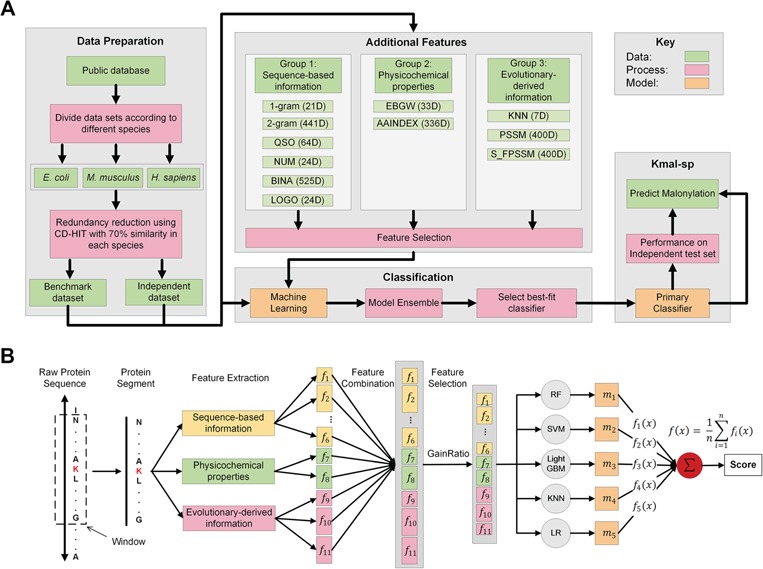
The overall framework of kmal-sp: (A) An outline of the overall flowchart of the kmal-sp methodology. (B) An illustration of the detailed procedures for constructing the prediction models for each species. First, the collected protein sequences are split into segments with a length (window size) of 25 residues each. Based on these segments, 11 different types of features are extracted that characterize Kmal sites in different aspects (these features are categorized into three main groups). Second, the optimal feature set is selected by applying the GainRatio method to the combined feature set. Based on the optimal feature set, we train the prediction models using several different ML algorithms and also exploit the integration of individual algorithm-based models into ensemble models. Finally, the optimal ensemble model is generated and applied to predict potential Kmal sites with improved accuracy.

Data collection and pre-processing

In this study, we used the data set in [13], which contains 9760 experimentally validated malonylation sites. This data set was originally collected from different public databases and works in the literature [7–10, 19–21]. The data set included 1746 Kmal sites from 595 E. coli proteins, 3435 Kmal sites from 1174 proteins in M. musculus and 4579 Kmal sites from 1660 proteins in H. sapiens. After downloading all abovementioned protein sequences from the UniProt database [22] using their UniProt IDs, Cluster Database at High Identity with Tolerance (CD-HIT) [23] was used to reduce the redundancy at the cutoff threshold of 70% sequence identity to avoid potential bias in model training. Then the processed sequences were truncated into 25-residue long sequence segments with lysine (K) located at the center. A segment was defined as a positive sample if its central K was malonylated, otherwise it was defined as a negative sample. After doing all of this, we obtained 1553, 2609 and 3885 positive samples and 7830, 26655 and 52027 negative samples for E. coli, M. musculus and H. sapiens, respectively (The data sets can be downloaded at http://kmalsp.erc.monash.edu/download.jsp/. Please refer to Table S2 for a statistical summary). The non-redundant data sets were randomly divided into the benchmark data sets and the independent data sets.

Feature extraction

Feature extraction directly affects the performance of constructed predictors. Features used in this work can be divided into three major groups: sequence-based features, physicochemical property-based features and evolutionary-derived features.

Group 1: sequence-based features

1-gram.

1-gram [11] is the specialization of k-grams [24] for which k is set to 1. In 1-gram, the relative frequencies of all 21 types of amino acids (20 standard amino acids and the dummy code O that fills the blank when the upstream or downstream in a segment is less than 12) are calculated using the following equation:

(1)

where denotes the number of amino acid r and N denotes the length of the segment (here N = 25). As a result, a 21-dimenstional vector would be obtained for each segment.

2-gram.

2-gram [11] calculates the relative frequencies of all possible dipeptides in the sequence. The elements of the feature vector are defined as

(2)

where denotes the count of the dipeptide rs, N denotes the length of the segment and N-1 represents the total number of dipeptides in the encoded segment. Consequently, a 441-dimensional vector would be obtained for each segment.

Quasi-sequence order.

The quasi-sequence-order (QSO) descriptor was originally proposed by Chou [25] and measures the occurrence of amino acids based on two distance matrices (i.e. the physicochemical distance matrix [26] and chemical distance matrix [27]). For a detailed description, refer to [25, 28]. We generated a 64-dimensional feature vector for each segment with parameter nlag of 12 [29].

Numerical representation for amino acids (NUM).

NUM aims to convert sequences of amino acids into sequences of numerical values as in [11] by mapping amino acids in an alphabetical order: the 20 standard amino acids are represented as 1, 2, 3,..., 20, and the dummy amino acid O is represented as 21. Here, each 25-residue segment, with the central residue K ignored, consists of 12 upstream residues, 12 downstream residues, thereby resulting in a 24-dimensional vector.

BINA.

The binary encoding of amino acids [13] converts each amino acid in a segment to a 21-dimensional orthogonal binary vector. Different from NUM described above, BINA represents each amino acid as a 21-dimensional binary vector encoded by one ‘1’ and 20 ‘0’ elements. For instance, alanine (‘A’) is represented as 100000000000000000000, cysteine (‘C’) is represented as 010000000000000000000,..., and so on, while the dummy amino acid ‘O’ is represented as 000000000000000000001. Consequently, we obtained a 525-dimensional vector for this BINA feature encoding, given the length of each segment is 25.

LOGO.

LOGO encodes a sequence segment based on the occurrence frequencies of amino acids as calculated by the Two Sample Logo program [30]. We chose the positive set and the negative set as inputs for Two Sample Logo and calculated the frequency of each amino acid at each specific position based on the differences between the positive and negative sets. At each position, we obtained frequencies for the 20 amino acid types. To calculate the feature vector for a target segment, the frequency of its amino acid at each position (24 positions in total, as the central residue K is ignored in this encoding scheme) was selected out as the element to generate a 24-dimensional feature vector for each 25-residue segment.

Group 2: physicochemical property-based features

Encoding based on grouped weight.

Encoding based on grouped weight (EBGW) [13] groups 20 amino acids into seven groups according to their hydrophobicity and charge characteristics (Table 1). For each group (i = 1, 2, 3), we generated a 25-dimensional array (i = 1, 2, 3), i.e. of the same length as that of the segment. An element in this array was set to 1 if the amino acid at that position belonged to the group and, otherwise, set to 0. Then, each array was divided into J sub-arrays, each of which (represented as ) can be obtained by slicing the original from the beginning with a window of len() (refer to the following equation):

Table 1.

Grouping of the 20 standard amino acids to four basic groups (C1–C4) and three combined groups (-) according to their hydrophobicity and charge characteristics

Group	Amino acids
Hydrophobic (C1)	A, F, G, I, L, M, P, V, W
Polar (C2)	C, N, Q, S, T, Y
Positively charged (C3)	K, H, R
Negatively charged (C4)	D, E
Combined	C1 + C2
Combined	C1 + C3
Combined	C1 + C4

(3)

where L refers to the length of the segment and the function int() rounds a decimal to the closest integer. For each group (i = 1, 2, 3), we accordingly obtained a vector with the length of J based on J sub-arrays, in which the j-th element can be calculated as follows:

(4)

where denotes the sum of the -th sub-array . In this study, we set J to 11 resulting in an 11*3 = 33-dimensional vector.

AAINDEX.

AAINDEX extracts features based on the amino acid indices from the AAIndex database [31], which has also been previously used for predicting malonylation sites [11]. For a segment (with length of 25 residues in this study), the amino acid at each position (except for the central K residue) is represented by 14 values according to physicochemical and biological properties, such as hydrophobicity, polarity, polarizability, slovent/hydration potential, accessibility reduction ratio, net charge index of side chains, molecular weight, PK-N, PK-C, melting point, optical rotation, entropy of formation, heat capacity and absolute entropy [11]. Accordingly, we obtained a 24  14 = 336-dimensional vector.

Group 3: evolutionary-derived features

KNN.

The KNN encoding generates features for each sequence segment based on its similarity to the k samples from both the positive and negative sets [13, 32]. For two segments and , the distance Dist() between and can be defined as

(5)

where l is the length of the segment and measures the similarity between the amino acids and based on the normalized amino acid substitution matrix. Such distance can be calculated as follows:

(6)

where a and b denote two amino acids, M is the substitution matrix (i.e. BLOSUM62 in this work) while max/min{M} represents the largest/smallest element value in the matrix, respectively. In this study, we used k with values of 2, 4, 8, 16, 32, 64 and 128 to generate a seven-dimensional vector for each segment.

Position-Specific Scoring Matrix based transformation (PSSM).

The evolutionary data in the form of Position-Specific Scoring Matrix (PSSM) profile are informative and have proved useful in a number of biological classification problems [28, 33–45]. In this work, the PSSM profile was generated by running PSI-BLAST against the uniref50 database with the parameters j = 3 and h = 0.001. For a segment with length = 25, the corresponding matrix of the PSSM profile has a size of 25 × 20. By summing up the rows that correspond with each amino acid [13, 46], the 25 × 20 matrix is transformed to a 20 × 20 matrix, resulting in a 400-dimensional feature vector.

S-FPSSM.

S-FPSSM [36] was first proposed to predict protein–protein interactions through row transformations of the original PSSM. In this work, we generated 400-dimensional S-FPSSM features by using the local POSSUM package developed to facilitate the processing and generation of PSSM-related features [41]. As a result, we generated 21 different types of PSSM features amongst which S-PFSSM achieved the most stable and accurate performance according to the benchmark test results.

Feature normalization

As mentioned above, in this study we applied 11 feature encoding methods to generate 2275-dimensional feature vectors. Original values of some features ranged from 0 to 0.01, others ranged from 0 to 500. We note use of features with large variations between intervals may lead to poor performance of trained models, a known issue for some ML algorithms, such as SVM. Therefore, to address this and improve the model performance, the original value of each feature was normalized to the [0, 1] range [47].

Feature selection

Heterogeneous features extracted from various points of view might be useful for characterizing Kmal sites; however, this will also lead to ‘feature explosion’ [48] and introduce redundancy and noise that can undermine model performance. To identify useful feature (sub-)sets from the initial feature set, we employed the GainRatio method, which is a feature selection method based on information theory [17]. The information entropy H(X) of a binary classification problem can be defined as

(7)

where P() denotes the probability of event taking on value (one of the two possible outcomes of the classification). The entropy of X after observing values of another variable is defined as

(8)

where m denotes the total number of features used. Finally, the formula of gain ratio is defined as

(9)

where GR denotes the gain ratio of the feature .

Model training

Random forest

RF [49] is a widely used ML algorithm with various successful applications in bioinformatics and computational biology [42, 50–52]. Assuming there exist N samples with M features in the original training set, RF selects N samples from the original training set by bootstrapping and randomly selects m (m <<M) features to train a decision tree. By repeating this procedure, many decision trees are trained and their outputs are aggregated in the ensemble model to generate the final prediction score of RF. Therefore, the numbers of decision trees and randomly selected features (mtry) are vital to the construction of accurate RF models. In this study, we trained the RF models with 1000 decision trees using the randomForest package [10] implemented in R with the parameter mtry optimized by its built-in function.

Support vector machine

As one of the most widely used ML algorithms applied to classification problems [11, 13, 14, 28, 35, 37, 39, 42, 53], SVM [54] maps the input data into a high-dimensional space through the use of kernel functions and finds a hyperplane that maximizes the distance between the hyperplane and two types of samples. By mapping the unseen samples into the same space, SVM can predict the new samples based on which side of the hyperplane they fall in. In this study, SVM with the Gaussian radial basis kernel was implemented using the e1071 package [55] in R. We optimized the parameters Cost C∈{, ,..., 1, , } and Gammaγ∈ {, ,..., 1, , } by grid search.

Gradient boosting decision tree

Gradient boosting decision tree (GBDT) [56] is an iterative decision tree-based algorithm with a number of effective implementations and extensions, such as Xgboost [57] and pGBRT [58], which has been widely used in bioinformatics and computational biology [59–61]. As a new implementation of GBDT with Gradient-based One-Side Sampling and Exclusive Feature Bundling, LightGBM has several attractive advantages including faster training speed, higher efficiency and lower memory usage, while still being able to achieve almost the same accuracy compared with Xgboost and pGBRT [62]. Here, we trained the LightGBM model using the LightGBM package in R language [62]. To improve the predictive performance of the models and avoid potential overfitting, we tuned 10 parameters (Table S3) by performing 10-time 10-fold cross-validation tests to maximize the area under the curve (AUC) values of the models.

K-nearest neighbor

The KNN algorithm measures the distances between a new sample and known samples in the training data set and predicts this new sample based on the majority vote of its closest k neighbors. As a simple and robust algorithm, KNN has been widely applied to solve various classification problems in bioinformatics [42, 59, 63, 64]. The parameter k of KNN has a significant impact on the performance of the K nearest neighbor algorithm. If k is too small, the classification result may be affected by outliers; if it is too large, the neighbors may contain too many types of points, reducing the prediction possibility of true positives. Empirically, k should be lower than the square root of the number of training samples. In this work, k was optimized at the range from 1 to 100, after taking the numbers (∼10 000) of training samples into consideration.

Logistic regression

Logistic regression is a classification algorithm based on statistics, which has been successfully applied to solve a number of classification tasks in bioinformatics [60, 65–67]. For logistic regression, the weight of independent variables can be calculated and then employed to make the prediction. In this study, logistic regression was implemented using the glm function implemented in the R language.

Randomized 10-fold cross-validation test

The 10-fold cross-validation test was used to evaluate the performance of different trained ML models. In 10-fold cross-validation, the benchmark data set is partitioned into 10 subsets. One subset is used as the test set and the others are used as the training sets. This procedure is conducted repeatedly, with each of the subsets being used once as the test set, to generate 10 models. The performance of the 10 corresponding results is averaged, which indicates the performance of the classifier. In this work, the 10-fold cross-validation test is further randomly conducted 10 times and the results are averaged as the final performance for trained models.

Independent test

To evaluate the performance of different models (both single method-based and ensemble models), we tested them on the independent test data sets. We also compared the performance of our models with the two existing state-of-the-art methods for malonylation site prediction, i.e. Mal-Lys [11] and MaloPred [13]. To make a fair and objective comparison with these two existing methods, we strictly implemented their algorithms and optimized parameters to build models on the same training data set and subsequently benchmark their performance on the independent test data sets.

Performance measures

To evaluate the performance of our proposed method, six measures including accuracy (ACC), specificity (SP), sensitivity (SN), precision (PRE), F-score and the Matthew’s correlation coefficient (MCC) were used. These are defined as follows:

(10)

(11)

(12)

(13)

(14)

(15)

where TP, TN, FP and FN represent the numbers of true positives, true negatives, false positives and false negatives, respectively. Moreover, the receiver operating characteristic (ROC) curves, together with the AUC are employed to comprehensively evaluate classification performance.

Experimental results

Sequence analysis

We analyzed the occurrence frequencies of amino acids at each position of the segments flanking the malonylation and non-malonylation sites in E. coli, M. musculus and H. sapiens. We used Two Sample Logo [30] with t-test (P < .05) with the purpose of examining whether the flanking sequence of Kmal sites could indeed possess differential patterns across species. As shown in Figure 2, lysine (K) is significantly enriched at multiple positions, especially 8–12 and 20–23, surrounding the Kmal sites, across all the three species. On the other hand, lysine (K) is depleted at certain positions downstream of the central Kmal sites (e.g. at positions 14 and 15) in both M. musculus and H. sapiens. Generally speaking, segments from E. coli and M. musculus share some common enriched patterns, in particular for lysine (K) (at positions 5–6, 8–12, 18 and 20–21) and arginine (R) (at positions 6–7, 18–19 and 20–21) residues. Interestingly, segments from M. musculus and H. sapiens share similar depleted amino acid occurrence patterns involving glutamic acid (E) (e.g. at positions 4, 8–12, 15, 17 and 21).

Figure 2.

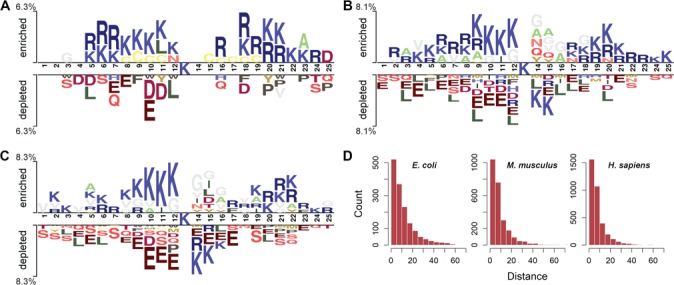
Sequence characteristics of Kmal sites across the three species. Panels (A), (B) and (C) illustrate the over-represented and under-represented amino acid occurrences in the segments flanking the central Kmal sites of E. coli, M. musculus and H. sapiens, respectively. Sequence logo representations were generated by Two Sample Logo with t-test (P < .05). Panel (D) represents distributions of the sequential distances between malonylation and non-malonylation segments within the same protein sequences.

As can be observed from Figure 2(A–C), the preference of lysine (K) at multiple positions flanking the central Kmal sites leads to an overlap between positive and negative segments to a large extent, thereby making it extremely challenging to accurately distinguish malonylation sites from non-malonylation sites. To further examine this overlap, we calculated distributions of the nearest sequential distances between non-malonylation and malonylation segments contained within the same protein sequences. The sequential distance between non-malonylation and malonylation segments could be measured by the relative distance between their central Ks. We thus analyzed the statistical distributions of sequential distances between non-malonylation and malonylation segments for E. coli, M. musculus and H. sapiens (Figure 2D). It can be observed that the distributions across all the three species have a very similar tendency, with more than half of the sequential distances being less than 10 amino acids long. This observation validates that there exists a huge overlap between the positive and negative segments and further highlights the challenges of extracting informative features based on sequence-based feature encodings, calling for more comprehensive and discriminative feature encoding methods for accurate prediction of malonylation sites.

Performance evaluation of different feature encoding schemes

We assessed the performance of 11 different feature encodings (categorized into three major groups) using RF based on 10-time 10-fold cross-validation tests (Figure 3, Figures S1–S3 and Tables S4–S6). Generally, we did not observe any single group of features outperforming other groups, for any species. The KNN features based on evolutionary information, LOGO features based on sequence information and AAINDEX features based on physicochemical properties are the three most important types of features that achieved the best performance for all the three species. This indicates the necessity and importance of exploiting effective combinations of feature types from various aspects, instead of using individual feature types alone, which have limited predictive power of the trained models. Specifically, as positive and negative segments often had overlapping sequence regions, traditional sequence-based feature coding methods, such as 1-gram, 2-gram, QSO, NUM and BINA, only achieved a poor performance. However, the new sequence encoding LOGO, although based on sequence information, achieved the best performance when compared with all other individual types of features within group 1 across the three species, demonstrating an enhanced capacity for discriminating the positive and negative samples.

Figure 3.

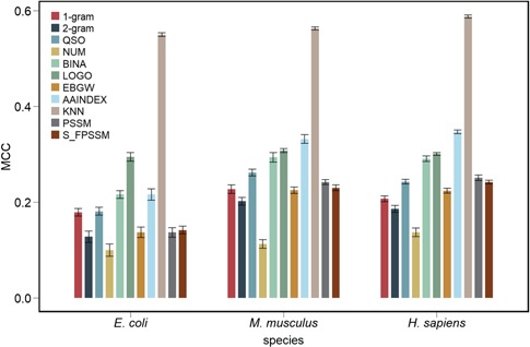
Performance comparison of the RF models trained using 11 different feature types based on 10-time 10-fold cross-validation tests for E. coli, M. musculus and H. sapiens. Randomized 10-fold cross-validation tests were conducted 10 times. The final performance of the RF models was averaged over the 10 times, with the standard error calculated and shown in bars.

For physicochemical property-based features, AAINDEX features outperformed EBGW features across all the three species in terms of ACC, F-value, MCC and AUC value. Surprisingly, the PSSM-based features showed poor performance, indicating a limited contribution to the prediction and a somewhat contrasting observation different from previous prediction studies of other protein attributes for which PSSM-based features are often considered essential [28, 36, 41, 42, 68–72]. A possible reason might be that part of the PSSM matrix used for describing the segment is far less informative than the complete PSSM matrix generated from full-length protein sequences in previous studies, thus making PSSM-based features unable to extract enough useful patterns and characteristics.

To further improve the predictive performance of the models, we combined the extracted features together to form a 2275-dimensional feature set, for each of the three species. By applying the GainRatio feature selection method to these full feature sets, we obtained species-specific rankings of feature sets. We then created and tested different feature sets that contained the top ranked features, ranging from the top 50 to the top 700 features, in intervals of 50. For each species, the selected feature sets were assessed: the corresponding performance results are shown in Figure 4 and Tables S7–S9. We note that, when gradually increasing the number of selected features, the performance of the models trained on the selected feature sets improved and then remained relatively stable for all the three species after reaching the peak. Moreover, most of the models trained on the selected feature sets achieved a better performance compared with those trained on the original (full) feature set. The overall best performance was achieved using 350, 350 and 500 top ranked features (labeled optimal feature sets) for E. coli, M. musculus and H. sapiens, respectively.

Figure 4.

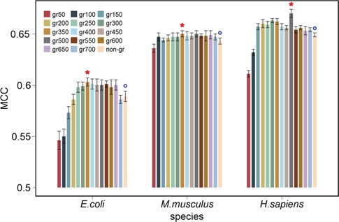
Performance comparison of RF models trained using different feature sets across the three species. Each feature set was assessed by applying GainRatio (‘gr’) to the original feature sets. Ten-fold cross-validation tests were randomly performed 10 times, and the performance was averaged with calculated standard deviations. Red stars denote the feature set with the overall best performance for the corresponding species, while blue circles represent the original feature set, prior to feature selection.

Next, we analyzed the compositions and distributions of different features in each optimal feature set. As shown in Figure 5(A–C), the feature distributions in the three optimal feature sets were largely similar but still had some subtle differences. Specifically, all KNN features and more than 50% of the LOGO features were selected and included in the optimal feature sets (Figure 5A–C (1)), suggesting their critical importance for Kmal site prediction. We also noticed that the AAINDEX features represent the largest proportion in the optimal feature sets for E. coli and M. musculus (Figure 5A and B (2/3)) and the 2nd largest for H. sapiens (Figure 5C (2/3)). It is also worth noting that PSSM-based features were the largest type of features (Figure 5C (2/3)) for H. sapiens but did not make a significant contribution to the predictive performance, reflected by the lower GainRatio score (Figure 5C (4)). To examine whether certain types of features are more relevant for predicting species-specific malonylation sites as compared with others, we further analyzed the GainRatio scores for the top 100 selected features in the optimal feature sets across the three species (Figure 5A–C (4)). The higher a feature’s GainRatio score is, the more important it is considered for its contribution to the predictor’s performance. As a result, we found that the KNN features accounted for the top two features in terms of GainRatio score for all three species. More specifically, the GainRatio score of the top KNN feature was larger than 0.3, which was more than twice the GainRatio score of many other features, stressing its importance for malonylation site prediction across all three species. Following the two KNN features, three AAINDEX features were ranked 3rd, 4th and 5th for E. coli, while the 1-gram features took the 3rd place for both M. musculus and H. sapiens and the 6th place for E. coli. This indicates that the 1-gram features also made a considerable contribution to malonylation site prediction across the three species, although this feature type has only 21 dimensions. On the other hand, we did not observe any particular feature type that was informative only for a single species. Overall, the KNN, AAINDEX, 1-gram and EBGW features contributed the most to malonylation site prediction for all the three species, suggesting that Kmal sites in the three species might share some common characteristics.

Figure 5.

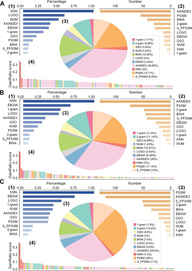
Distribution analysis of generated optimal feature sets across the three species. Panels (A), (B) and (C) illustrate distributions of feature types included in the optimal feature sets for E. coli, M. musculus and H. sapiens, respectively. In each panel (A, B and C), (1) and (2) show the percentage and the number, respectively, of each feature type selected in the optimal feature set, (3) depicts the proportion of the types of features selected in the optimal feature set while (4) provides the GainRatio score for the top 100 selected features in the optimal feature set.

Performance evaluation of different single ML method-based models and their ensemble models

By using the optimal feature sets of the three species, we first built models based on five different ML methods and compared their performance by performing 10 rounds of 10-fold cross-validation tests. As shown in Table 2, RF, SVM and the recently developed LightGBM method [62] achieved overall the best performances for all three species. Among these ML methods, with increasing size of the training/learning data sets (E. coli < M. musculus < H. sapiens), the performance of RF appeared to be more stable than that of SVM. This observation is consistent with the conclusion drawn in a previous study [73], where the authors found that RF is more suitable for larger data sets with a desirable robustness property while SVM is more suitable for relatively smaller data sets that contain fewer ‘extreme’ values. In contrast to the two aforementioned ML methods, LightGBM achieved both best performance and computational efficiency when being applied to the largest data set (i.e. H. sapiens). This is attributable to its specific design advantage that makes itself particularly suitable for industrial-scale mass data processing and parallel computing [62].

Table 2.

Performance comparison of five single ML method-based models to predict malonylation sites for the three species using 10-fold cross-validation tests. Ten-fold cross-validation tests were randomly performed 10 times, and the reported performance is the average of the individual performances

Species	Method	PRE	SN	SP	F-value	ACC	MCC
E. coli	RF	0.787 ± 0.002	0.826 ± 0.004	0.776 ± 0.002	0.805 ± 0.002	0.801 ± 0.002	0.603 ± 0.004
SVM	0.813 ± 0.003	0.810 ± 0.003	0.813 ± 0.005	0.811 ± 0.002	0.812 ± 0.002	0.624 ± 0.004
LightGBM	0.785 ± 0.004	0.815 ± 0.007	0.776 ± 0.005	0.799 ± 0.004	0.796 ± 0.004	0.592 ± 0.007
KNN	0.826 ± 0.005	0.699 ± 0.003	0.853 ± 0.004	0.756 ± 0.003	0.776 ± 0.003	0.558 ± 0.006
LR	0.792 ± 0.005	0.795 ± 0.005	0.791 ± 0.006	0.793 ± 0.004	0.793 ± 0.004	0.586 ± 0.009
M. musculus	RF	0.818 ± 0.002	0.835 ± 0.003	0.815 ± 0.002	0.826 ± 0.002	0.825 ± 0.002	0.650 ± 0.003
SVM	0.833 ± 0.002	0.832 ± 0.002	0.833 ± 0.002	0.832 ± 0.002	0.832 ± 0.002	0.665 ± 0.004
LightGBM	0.826 ± 0.002	0.836 ± 0.004	0.824 ± 0.003	0.830 ± 0.003	0.830 ± 0.002	0.659 ± 0.005
KNN	0.848 ± 0.002	0.721 ± 0.004	0.871 ± 0.003	0.779 ± 0.002	0.796 ± 0.002	0.599 ± 0.003
LR	0.822 ± 0.003	0.820 ± 0.003	0.822 ± 0.004	0.820 ± 0.002	0.821 ± 0.002	0.641 ± 0.005
H. sapiens	RF	0.838 ± 0.002	0.830 ± 0.003	0.840 ± 0.002	0.834 ± 0.002	0.835 ± 0.002	0.670 ± 0.004
SVM	0.832 ± 0.002	0.825 ± 0.002	0.834 ± 0.002	0.828 ± 0.001	0.829 ± 0.001	0.659 ± 0.002
LightGBM	0.837 ± 0.003	0.833 ± 0.004	0.838 ± 0.003	0.835 ± 0.003	0.835 ± 0.003	0.671 ± 0.005
KNN	0.835 ± 0.002	0.752 ± 0.003	0.851 ± 0.002	0.791 ± 0.002	0.801 ± 0.002	0.606 ± 0.004
LR	0.824 ± 0.002	0.819 ± 0.003	0.825 ± 0.002	0.821 ± 0.002	0.822 ± 0.002	0.644 ± 0.004

Note: Performances are shown as mean ± standard deviation. For each species, the best performance (as measured by each metric) across different encoding methods is highlighted in bold for clarification. For each performance metric, the best performance value across different machine learning methods within a species is highlighted in bold for clarification. These highlights also apply to Tables 3 and 4.

Next, we investigated the performance of the single method-based models on the independent test. As shown in Table 3, the prediction performance is highly consistent with the results from the 10-fold cross-validation tests as discussed above, further validating the robustness and generalization ability of these models. We also constructed ensemble models from single models and evaluated their performances. The final prediction score of the ensemble model was calculated by averaging all individual single models’ outputs, using equal weights. Table 3 indicates the ensemble model with the best performance over all possible combinations of up to five single models. Several observations can be made: (i) The performance of the ensemble model did not show a correlation with the number of single method-based models. For all three species, the optimal models were not the ensemble models integrating all single models. In fact, the performance of ensemble models based on all single models was slightly lower than that of the best single model in the case of M. musculus and H. sapiens. However, the ensemble models often outperformed the majority of single models and thus can still offer more stable prediction results [42, 74, 75]. (ii) The ensemble models that integrated several top-performing single method-based models, i.e. the ensemble model {1, 2} for M. musculus and the ensemble models {1, 2, 3} and {1, 2, 3, 4} for H. sapiens, did not achieve significant performance improvements. (iii) The best performing ensemble models combine methods with moderate performance, such as KNN and LR, with other top-performing methods. For example, the optimal ensemble model {1, 3, 4} for E. coli combines KNN with the two top-performing methods RF and LightGBM. Similar performance results could also be observed for the other two species, which provides useful insights when considering constructing better ensemble models.

Table 3.

Performance comparison of different single method-based models and a selection of ensemble models for predicting malonylation sites of the three species on the independent test

Species	Method a	PRE	SN	SP	F-value	ACC	MCC
E. coli	1. RF	0.828	0.820	0.830	0.824	0.825	0.650
2. SVM	0.798	0.790	0.800	0.794	0.795	0.590
3. LightGBM	0.806	0.830	0.800	0.818	0.815	0.630
4. KNN	0.862	0.750	0.880	0.802	0.815	0.635
5. LR	0.814	0.790	0.820	0.802	0.805	0.610
{1, 2}	0.842	0.800	0.850	0.821	0.825	0.651
{1, 2, 3}	0.830	0.830	0.830	0.830	0.830	0.660
{1, 2, 3, 4}	0.845	0.820	0.850	0.832	0.835	0.670
{1, 2, 3, 4, 5}	0.840	0.790	0.850	0.814	0.820	0.641
{1, 3, 4} *	0.856	0.830	0.860	0.843	0.845	0.690
M. musculus	1. RF	0.810	0.843	0.804	0.826	0.823	0.647
2. SVM	0.818	0.829	0.817	0.824	0.823	0.647
3. LightGBM	0.810	0.826	0.807	0.818	0.817	0.633
4. KNN	0.810	0.729	0.831	0.768	0.780	0.563
5. LR	0.808	0.829	0.804	0.818	0.817	0.634
{1, 2}	0.821	0.826	0.821	0.823	0.823	0.647
{1, 2, 3}	0.807	0.823	0.804	0.815	0.813	0.627
{1, 2, 3, 4}	0.826	0.839	0.824	0.833	0.832	0.663
{1, 2, 3, 4, 5}	0.828	0.836	0.827	0.832	0.832	0.663
{1, 2, 4} *	0.835	0.829	0.837	0.832	0.833	0.667
H. sapiens	1. RF	0.834	0.843	0.834	0.839	0.838	0.677
2. SVM	0.837	0.839	0.837	0.838	0.838	0.677
3. LightGBM	0.854	0.863	0.854	0.859	0.858	0.717
4. KNN	0.833	0.749	0.850	0.789	0.800	0.603
5. LR	0.840	0.823	0.844	0.831	0.833	0.667
{1, 2}	0.855	0.846	0.857	0.850	0.852	0.703
{1, 2, 3}	0.855	0.846	0.857	0.850	0.852	0.703
{1, 2, 3, 4}	0.863	0.846	0.867	0.855	0.857	0.713
{1, 2, 3, 4, 5}	0.863	0.846	0.867	0.855	0.857	0.713
{3, 4, 5} *	0.867	0.849	0.870	0.858	0.860	0.720

^{a a}Each item in this column refers to a single method-based model or an ensemble model that was built based on combining different single models (e.g. ‘1. RF’ means the model is trained based on RF, while ‘{1, 2}’ stands for the ensemble model that is built based on combining the single models numbered ‘1’ and ‘2’).

^{* *}The optimal ensemble model was selected by exhaustively examining all possible random combinations of up to five single models.

Performance comparison with existing state-of-the-art methods

Since malonylations were only recently discovered, currently only three tools exist for predicting malonylation sites. The earliest tool, Mal-lys, was only trained using mouse data [11]. A most recent tool, MaloPred [13], can predict potential malonylation sites for the three species (E. coli, M. musculus and H. sapiens), while SPRINT-Mal [15] is able to predict malonylation sites for H. sapiens and M.musculus. Because of a large overlap between our data sets and theirs, it is difficult to construct independent test data sets that do not intersect with their training data sets. Therefore, to make a fair and objective comparison, we trained their classifiers based on our training data sets by strictly following their methods and assessed and compared performance of their methods and our proposed method based on the independent test data sets. As the source codes of SPRINT-Mal were not available, in this section, we compared our method (kmal-sp) with the other two existing tools MaloPred and Mal-lys. The performance comparison results between kmal-sp and MaloPred (which provided a better performance compared with Mal-lys) are shown in Table 4 and Figure 6.

Table 4.

Performance comparison between our proposed method and the state-of-the-art method MaloPred for predicting malonylation sites of the three species based on the independent test

Species	Method	PRE	SN	SP	F-value	ACC	MCC
E. coli	kmal-sp	0.856	0.830	0.860	0.843	0.845	0.690
MaloPred	0.798	0.750	0.810	0.773	0.780	0.561
M. musculus	kmal-sp	0.835	0.829	0.837	0.832	0.833	0.667
MaloPred	0.798	0.806	0.797	0.802	0.802	0.603
H. sapiens	kmal-sp	0.867	0.849	0.870	0.858	0.860	0.720
MaloPred	0.824	0.829	0.824	0.827	0.827	0.653

Figure 6.

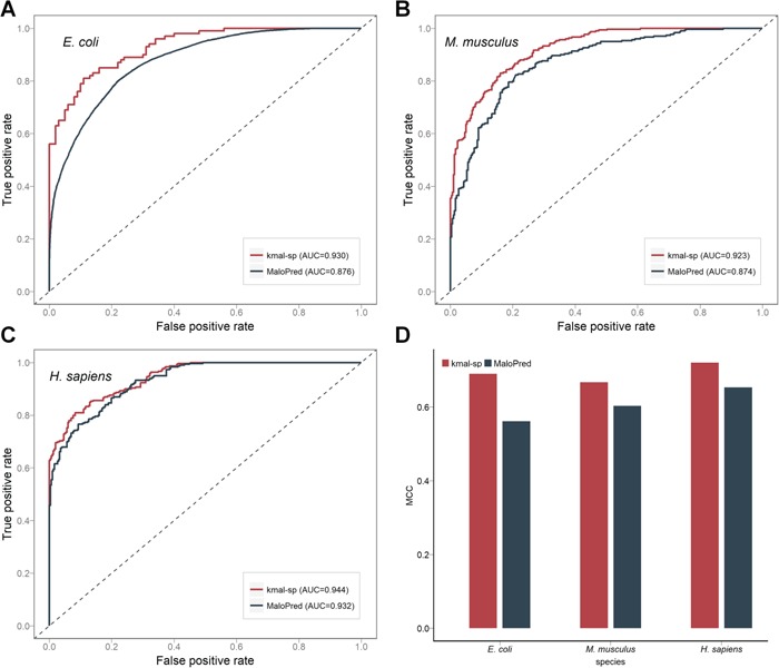
Performance comparison between our proposed method kmal-sp and the state-of-the-art method MaloPred for predicting malonylation sites. (A), (B) and (C) ROC curves of both methods on the independent test for predicting malonylation sites of E. coli, M. musculus, and H. sapiens, respectively. (D) histograms showing the performance of kmal-sp and MaloPred in terms of MCC on the independent test.

As shown in Table 4 and Figure 6D, kmal-sp clearly outperformed MaloPred across all the three species in terms of all the major metrics, including PRE, SN, SP, ACC, F-value and MCC. In addition, we also plotted ROC curves (Figure 6A–C) that provide a comprehensive performance comparison between the two methods. The reasons why kmal-sp provided a better performance than MaloPred are: first, kmal-sp used an enlarged set of informative sequence-based features. As discussed in the Section Sequence Analysis, because of the higher similarity between the positive and the negative data, traditional feature encodings (e.g. AAC) based on basic sequence information achieve a poorer performance. In contrast, Kmal-sp used sequence-based information from three complementary points of view including amino acid occurrence probability (encoded by 1-gram, 2-gram and QSO), amino acid numerical encodings (BINA and NUM) and encodings that take into consideration the position-specific difference between the positive and negative segments (encoded by LOGO); In addition, 14 additional physicochemical property-based features were also considered by the AAINDEX encoding, which indeed showed an excellent predictive performance in [11] and also confirmed in this work; second, we benchmarked the performance of five state-of-the-art ML algorithms and built kmal-sp to exploit optimal ensemble modeling, leading to even more accurate predictions of malonylation sites.

Availability of online web server

To facilitate the community-wide prediction of malonylation sites, we have implemented an online web server of kmal-sp based on the optimal ensemble models for the three species. Kmal-sp is a user-friendly application available at and hosted by Monash’s extensible cloud computing facility with 16-core processors, 64 GB memory and 2 TB disk. It is publicly accessible at http://kmalsp.erc.monash.edu/.

The user submission interface (Figure 7A) allows users to directly input the query protein sequences or upload the data set by clicking the Browse button (both in the FASTA format). After selecting the predicted species and specifying the prediction cutoff value, users can click the Submit button to initiate processing of their tasks. Users can then check the processing status of the submitted jobs using a unique URL link or, alternatively, receive an automatic e-mail notification once their tasks are completed if they choose to provide an e-mail address for this purpose. For illustration purposes, we provide a screenshot of the prediction result web page in Figure 7B. From the result web page users can download the prediction result in multiple formats, allowing subsequent in-depth analysis on their local computers.

Figure 7.

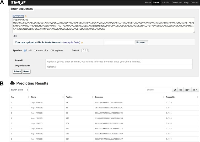
Screenshot of the online web server kmal-sp: (A) the user submission interface and (B) the predicted result for a case study protein sequence as input.

Discussion and conclusions

Identifying Kmal sites is pivotal to understanding the regulation mechanisms of glycolipid metabolism [10]. Although there have been some computational efforts to predict Kmal sites, a systematic analysis and comprehensive assessment of the informative features, usefulness of ML methods and their potential integration have been lacking.

In this work, we have systematically analyzed, benchmarked and compared 11 different types of feature encoding methods categorized in three major groups, by using RF-based ML models. Features were carefully selected according to their evaluated effectiveness for predicting Kmal sites. Using the benchmark data sets of the three species E. coli, M. musculus and H. sapiens, we have obtained optimized feature sets for each species based on feature selection. Using these optimized feature sets, different prediction models were trained using additional four ML methods (including classical and recently proposed ML methods) and rigorously evaluated using both 10 runs of 10-fold cross-validation and independent tests. Moreover, we explored the integration of these single ML method-based models into ensemble strategies and showed that these strategies can further improve the prediction performance and robustness of the model. The optimal ensemble models outperformed current state-of-the-art predictors for identifying Kmal sites on the independent data sets across the three different species. Lastly, we have developed a user-friendly web server called kmal-sp based on our optimal ensemble models, for use by the wider research community. As complementary and heterogeneous features extracted from different perspectives can be generally helpful for improving the predictors’ performance, we will continually make an effort to explore more informative features, examine their contribution and refine our prediction platform. Furthermore, features that have been successfully applied to predict other types of protein PTM sites, such as structural property-based features in phosphorylation site prediction [52, 76], might also prove useful toward improving Kmal site prediction. We will continue to exploit such new features and update the prediction models, continuously improving the webserver to better serve users’ needs.

We anticipate that our findings, the proposed computational framework, integration and ensemble strategy, together with the continued development of our online web server, will instill a new momentum for bioinformatics studies of Kmal sites and other functionally important PTM types, as well as inspire users to develop novel computational methods. Such efforts and studies will continually make a contribution to improving our understanding of the important determinants of protein PTMs and facilitating their discovery.

Key Points

• This work provides a systematic comparison of 11 feature encoding methods in identifying Kmal sites. For each of three species, we investigated the relative utility of all resulting features and identified best-performing features sets.

• Using the optimized feature sets, five different machine learning methods were trained and compared on a rigorous benchmark test.

• Comparative analysis of individual machine learning models and their integrations revealed that ensemble models exhibit an improved predictive performance. The optimal ensemble models outperformed current state-of-the-art malonylation site predictors on the independent test data sets across different species.

• We accordingly implemented a user-friendly web server called kmal-sp, based on the optimal ensemble models, to facilitate community-wide efforts toward identifying novel malonylation substrates and sites, which is freely accessible at http://kmalsp.erc.monash.edu/.

Yanju Zhang received her PhD degree at the Leiden Institute of Advanced Computer Science, Leiden University, the Netherlands, in 2011. She is currently a professor and the head of Bioinformatics Group at the School of Computer Science and Information Security, Guilin University of Electronic Technology, China. Her research interests are bioinformatics, algorithms and modeling, machine learning, data mining and precision medicine

Ruopeng Xie is currently a master student in the School of Computer Science and Information Security, Guilin University of Electronic Technology, China. He received his bachelor degree in computer science and technology from Shanghai Business School. His research interests are bioinformatics, machine learning and data mining

Jiawei Wang is currently a PhD candidate in the Biomedicine Discovery Institute and the Department of Microbiology at Monash University, Australia. He received his bachelor degree in software engineering from Tongji University and his master degree in computer science from Peking University, China. His research interests are computational biology, bioinformatics, machine learning and data mining

André Leier is currently an assistant professor in the Department of Genetics, University of Alabama at Birmingham (UAB) School of Medicine, USA. He is also an associate scientist in the UAB Comprehensive Cancer Center. He received his PhD in Computer Science (Dr. rer. Nat.), University of Dortmund, Germany. He conducted postdoctoral research at Memorial University of Newfoundland, Canada; The University of Queensland, Australia; and ETH Zürich, Switzerland. His research interests are in Biomedical Informatics and Computational and Systems Biomedicine

Tatiana T. Marquez-Lago is an associate professor in the Department of Genetics and the Department of Cell, Developmental and Integrative Biology, UAB School of Medicine, USA. Her research interests include multiscale modeling and simulations, artificial intelligence, bioengineering and systems biomedicine. Her interdisciplinary laboratory studies stochastic gene expression, chromatin organization, antibiotic resistance in bacteria and host-microbiota interactions in complex diseases

Tatsuya Akutsu received his DEng degree in Information Engineering in 1989 from University of Tokyo, Japan. Since 2001, he has been a professor in the Bioinformatics Center, Institute for Chemical Research, Kyoto University, Japan. His research interests include bioinformatics and discrete algorithms

Geoffrey I. Webb received his PhD degree in 1987 from La Trobe University, Australia. He is a professor in the Faculty of Information Technology and director of the Monash Centre for Data Science at Monash University. His research interests include machine learning, data mining, computational biology and user modeling

Kuo-Chen Chou received his DSc degree in 1984 from Kyoto University, Japan. He is the founder and chief scientist of Gordon Life Science Institute. He is also a Distinguished High Impact Professor and advisory professor of several universities. His research interests are computational biology and biomedicine, protein structure prediction, low-frequency internal motion of protein/DNA molecules and its biological functions, diffusion-controlled reactions of enzymes as well as graphic rules in enzyme kinetics and other biological systems

Jiangning Song is a senior research fellow and group leader in the Biomedicine Discovery Institute and the Department of Biochemistry and Molecular Biology, Monash University, Melbourne, Australia. He is a member of the Monash Centre for Data Science, Monash University. He is also an associate investigator at the ARC Centre of Excellence in Advanced Molecular Imaging, Monash University. His research interests include bioinformatics, systems biology, machine learning, functional genomics and enzyme engineering

Funding

This work was supported by the Natural Science Foundation of Guangxi (2016GXNSFCA380005), Innovation Project of Guilin University of Electronic Technology Graduate Education (2018YJCX49), the Australian Research Council (ARC) (LP110200333 and DP120104460), the National Institute of Allergy and Infectious Diseases of the National Institutes of Health (R01 AI111965) and a Major Inter-Disciplinary Research project awarded by Monash University. G.I.W. is a recipient of the Discovery Outstanding Research Award (DP140100087) of the ARC. T.T.M.L. and A.L.’s work was supported in part by the Informatics Institute of the School of Medicine at University of Alabama at Birmingham.

References

- 1. Gallego M, Virshup DM. Post-translational modifications regulate the ticking of the circadian clock. Nat Rev Mol Cell Biol 2007;8:139–48. [DOI] [PubMed] [Google Scholar]
- 2. Westermann S, Weber K. Post-translational modifications regulate microtubule function. Nat Rev Mol Cell Biol 2003;4:938–47. [DOI] [PubMed] [Google Scholar]
- 3. Harmel R, Fiedler D. Features and regulation of non-enzymatic post-translational modifications. Nat Chem Biol 2018;14:244–52. [DOI] [PubMed] [Google Scholar]
- 4. Johnson LN. The regulation of protein phosphorylation. Biochem Soc Trans 2009;37:627–41. [DOI] [PubMed] [Google Scholar]
- 5. Ambler RP, Rees MW. Epsilon-N-Methyl-lysine in bacterial flagellar protein. Nature 1959;183:1654–5. [DOI] [PubMed] [Google Scholar]
- 6. Roth SY, Denu JM, Allis CD. Histone acetyltransferases. Annu Rev Biochem 2001;70. [DOI] [PubMed] [Google Scholar]
- 7. Xie Z, Dai J, Dai L, et al. Lysine succinylation and lysine malonylation in histones. Mol Cell Proteomics 2012;11:100–7. [DOI] [PMC free article] [PubMed] [Google Scholar]
- 8. Hirschey MD, Zhao Y. Metabolic regulation by lysine malonylation, succinylation, and glutarylation. Mol Cell Proteomics 2015;14:2308–15. [DOI] [PMC free article] [PubMed] [Google Scholar]
- 9. Peng C, Lu Z, Xie Z, et al. The first identification of lysine malonylation substrates and its regulatory enzyme. Mol Cell Proteomics 2011;10:M111.012658. [DOI] [PMC free article] [PubMed] [Google Scholar]
- 10. Du Y, Cai T, Li T, et al. Lysine malonylation is elevated in type 2 diabetic mouse models and enriched in metabolic associated proteins. Mol Cell Proteomics 2015;14(1):227–36. [DOI] [PMC free article] [PubMed] [Google Scholar]
- 11. Xu Y, Ding Y, Ding J, et al. Mal-Lys: prediction of lysine malonylation sites in proteins integrated sequence-based features with mRMR feature selection. Nat Publ Gr 2016;1–7. [DOI] [PMC free article] [PubMed] [Google Scholar]
- 12. Du Y, Zhai Z, Li Y, et al. Prediction of protein lysine acylation by integrating primary sequence information with multiple functional features. J Proteome Res 2016;15:4234–44. [DOI] [PubMed] [Google Scholar]
- 13. Wang LN, Shi SP, Xu HD, et al. Computational prediction of species-specific malonylation sites via enhanced characteristic strategy. Bioinformatics 2017;33:1457–63. [DOI] [PubMed] [Google Scholar]
- 14. Xiang Q, Feng K, Liao B, et al. Prediction of lysine malonylation sites based on pseudo amino acid compositions. Comb Chem. High Throughput Screen 2017;20:1. [DOI] [PubMed] [Google Scholar]
- 15. Taherzadeh G, Yang Y, Xu H, et al. Predicting lysine-malonylation sites of proteins using sequence and predicted structural features. J Comput Chem 2018, 10.1002/jcc.25353. [DOI] [PubMed] [Google Scholar]
- 16. Peng H, Long F, Ding C. Feature selection based on mutual information: criteria of max-dependency, max-relevance, and min-redundancy. IEEE Trans Pattern Anal Mach Intell 2005;27:1226–38. [DOI] [PubMed] [Google Scholar]
- 17. Shannon CE. A mathematical theory of communication: the bell system technical journal. Bell Syst Tech J 1948 1948;27(3):1948. [Google Scholar]
- 18. Chou KC. Some remarks on protein attribute prediction and pseudo amino acid composition. J Theor Biol 2011;273:236–47. [DOI] [PMC free article] [PubMed] [Google Scholar]
- 19. Qian L, Nie L, Chen M, et al. Global profiling of protein lysine malonylation in Escherichia coli reveals its role in energy metabolism. Proteome Res 2016;15:2060–71. [DOI] [PubMed] [Google Scholar]
- 20. Colak G, Pougovkina O, Dai L, et al. Proteomic and biochemical studies of lysine malonylation suggest its malonic aciduria-associated regulatory role in mitochondrial function and fatty acid oxidation. Mol Cell Proteomics 2015;14:3056–71. [DOI] [PMC free article] [PubMed] [Google Scholar]
- 21. Nishida Y, Rardin MJ, Carrico C, et al. SIRT5 regulates both cytosolic and mitochondrial protein malonylation with glycolysis as a major target. Mol Cell 2016;59:321–32. [DOI] [PMC free article] [PubMed] [Google Scholar]
- 22. Apweiler R, Martin MJ, O’Donovan C, et al. Ongoing and future developments at the Universal Protein Resource. Nucleic Acids Res 2011;39:214–9. [DOI] [PMC free article] [PubMed] [Google Scholar]
- 23. Huang Y, Niu B, Gao Y, et al. CD-HIT suite: a web server for clustering and comparing biological sequences. Bioinformatics 2010;26:680–2. [DOI] [PMC free article] [PubMed] [Google Scholar]
- 24. Liu H, Wong L. Data mining tools for biological sequences. J Bioinform Comput Biol 2003;1:139–67. [DOI] [PubMed] [Google Scholar]
- 25. Chou KC. Prediction of protein subcellular locations by incorporating quasi-sequence-order effect. Biochem Biophys Res Commun 2000;278:477–83. [DOI] [PubMed] [Google Scholar]
- 26. Schneider G, Wrede P. The rational design of amino acid sequences by artificial neural networks and simulated molecular evolution: de novo design of an idealized leader peptidase cleavage site. Biophys J 1994;66:335–44. [DOI] [PMC free article] [PubMed] [Google Scholar]
- 27. Grantham R. Amino acid difference formula to help explain protein evolution. Science 1974;185:862–4. [DOI] [PubMed] [Google Scholar]
- 28. Wang J, Yang B, Leier A, et al. Bastion6: a bioinformatics approach for accurate prediction of type VI secreted effectors. Bioinformatics 2018;34(15):2546–55. [DOI] [PMC free article] [PubMed] [Google Scholar]
- 29. Xiao N, Cao DS, Zhu MF, et al. Protr/ProtrWeb: R package and web server for generating various numerical representation schemes of protein sequences. Bioinformatics 2015;31:1857–9. [DOI] [PubMed] [Google Scholar]
- 30. Vacic V, Iakoucheva LM, Radivojac P. Two sample logo: a graphical representation of the differences between two sets of sequence alignments. Bioinformatics 2006;22:1536–7. [DOI] [PubMed] [Google Scholar]
- 31. Kawashima S, Pokarowski P, Pokarowska M, et al. AAindex: amino acid index database, progress report 2008. Nucleic Acids Res 2008;36:202–5. [DOI] [PMC free article] [PubMed] [Google Scholar]
- 32. Gao J, Thelen JJ, Dunker AK, et al. Musite, a tool for global prediction of general and kinase-specific phosphorylation sites. Mol Cell Proteomics 2010;9:2586–600. [DOI] [PMC free article] [PubMed] [Google Scholar]
- 33. Liu T, Tao P, Li X, et al. Prediction of subcellular location of apoptosis proteins combining tri-gram encoding based on PSSM and recursive feature elimination. J Theor Biol 2015;366:8–12. [DOI] [PubMed] [Google Scholar]
- 34. Wang J, Wang C, Cao J, et al. Prediction of protein structural classes for low-similarity sequences using reduced PSSM and position-based secondary structural features. Gene 2015;554:241–8. [DOI] [PubMed] [Google Scholar]
- 35. Chen Y, Liu Y, Cheng J, et al. Prediction of protein secondary structure using SVM-PSSM classifier combined by sequence features. 2016 IEEE Adv Inf Manag Commun Electron Autom Control Conf 2016;103–6. [Google Scholar]
- 36. Zahiri J, Yaghoubi O, Mohammad-Noori M, et al. PPIevo: Protein-protein interaction prediction from PSSM based evolutionary information. Genomics 2013;102:237–42. [DOI] [PubMed] [Google Scholar]
- 37. Kumar M, Gromiha MM, Raghava GPS. Prediction of RNA binding sites in a protein using SVM and PSSM profile. Proteins 2008;71:189–4. [DOI] [PubMed] [Google Scholar]
- 38. Zhai JX, Cao TJ, An JY, et al. Highly accurate prediction of protein self-interactions by incorporating the average block and PSSM information into the general PseAAC. Theor Biol 2017;432:80–6. [DOI] [PubMed] [Google Scholar]
- 39. Kurniawan I, Haryanto T, Hasibuan LS, et al. Combining PSSM and physicochemical feature for protein structure prediction with support vector machine. J Phys Conf Ser 2017;835:012006. [Google Scholar]
- 40. Li Z-W, You Z-H, Chen X, et al. Accurate prediction of protein-protein interactions by integrating potential evolutionary information embedded in PSSM profile and discriminative vector machine classifier. Oncotarget 2017;8:23638–49. [DOI] [PMC free article] [PubMed] [Google Scholar]
- 41. Wang J, Yang B, Revote J, et al. POSSUM: a bioinformatics toolkit for generating numerical sequence feature descriptors based on PSSM profiles. Bioinformatics 2017;33:2756–8. [DOI] [PubMed] [Google Scholar]
- 42. Wang J, Yang B, An Y, et al. Systematic analysis and prediction of type IV secreted effector proteins by machine learning approaches. Brief Bioinform 2017, 10.1093/bib/bbx164. [DOI] [PMC free article] [PubMed] [Google Scholar]
- 43. Song J, Burrage K, Yuan Z, et al. Prediction of cis/trans isomerization in proteins using PSI-BLAST profiles and secondary structure information. BMC Bioinformatics 2006;7:1–13. [DOI] [PMC free article] [PubMed] [Google Scholar]
- 44. Chen K, Kurgan L. PFRES: Protein fold classification by using evolutionary information and predicted secondary structure. Bioinformatics 2007;23:2843–50. [DOI] [PubMed] [Google Scholar]
- 45. Song J, Yuan Z, Tan H, et al. Predicting disulfide connectivity from protein sequence using multiple sequence feature vectors and secondary structure. Bioinformatics 2007;23:3147–54. [DOI] [PubMed] [Google Scholar]
- 46. Zou L, Nan C, Hu F, et al. Accurate prediction of bacterial type IV secreted effectors using amino acid composition and PSSM profiles. Bioinformatics 2013;29:3135–42. [DOI] [PMC free article] [PubMed] [Google Scholar]
- 47. Aksoy S, Haralick RM. Feature Normalization and Likelihood-based Similarity Measures for Image Retrieval. Pattern recognition letters 2001;22(5):563–82. [Google Scholar]
- 48. Guyon I, Elisseeff A. An introduction to variable and feature selection. J Mach Learn Res 2003;3:1157–82. [Google Scholar]
- 49. Breiman L. Random forests. Mach Learn 2001;45:5–32. [Google Scholar]
- 50. An Y, Wang J, Li C, et al. Comprehensive assessment and performance improvement of effector protein predictors for bacterial secretion systems III, IV and VI. Brief Bioinform 2018;19(1):148–61. [DOI] [PubMed] [Google Scholar]
- 51. Song J, Li F, Takemoto K, et al. PREvaIL, an integrative approach for inferring catalytic residues using sequence, structural, and network features in a machine-learning framework. J Theor Biol 2018;443:125–37. [DOI] [PubMed] [Google Scholar]
- 52. Song J, Wang H, Wang J, et al. PhosphoPredict: a bioinformatics tool for prediction of human kinase-specific phosphorylation substrates and sites by integrating heterogeneous feature selection. Sci Rep 2017;7:6862. [DOI] [PMC free article] [PubMed] [Google Scholar]
- 53. Kumar M, Gromiha MM, Raghava GPS. SVM based prediction of RNA-binding proteins using binding residues and evolutionary information. J Mol Recognit 2011;24:303–13. [DOI] [PubMed] [Google Scholar]
- 54. Noble WS. What is a support vector machine? Nat. Biotechnol. 2006;24:1565–7. [DOI] [PubMed] [Google Scholar]
- 55. Meyer D, Dimitriadou E, Hornik K, et al. e1071: Misc Functions of the Department of Statistics. Probab. Theory Gr. (Formerly E1071) R Packag. version 1.6-7, 2015.
- 56.Friedman JH. Greedy function approximation a gradient boosting machine. Ann Stat 2001;29(5):1189–232. [Google Scholar]
- 57. Chen T, Guestrin C. Xgboost: A scalable tree boosting system. In: Proceedings of the 22nd acm sigkdd international conference on knowledge discovery and data mining, 2016;785–94. [Google Scholar]
- 58. Tyree S, Weinberger KQ, Agrawal K, et al. Parallel boosted regression trees for web search ranking. Proceedings of the 20th International Conference on World wide web; Hyderabad, India 2011;387. [Google Scholar]
- 59. Liao Z, Huang Y, Yue X, et al. In silico prediction of gamma-aminobutyric acid type-a receptors using novel machine-learning-based SVM and GBDT approaches. Biomed Res Int 2016;2016. [DOI] [PMC free article] [PubMed] [Google Scholar]
- 60. Ichikawa D, Saito T, Ujita W, et al. How can machine-learning methods assist in virtual screening for hyperuricemia? A healthcare machine-learning approach. J Biomed Inform 2016;64:20–4. [DOI] [PubMed] [Google Scholar]
- 61. Rawi R, Mall R, Kunji K, et al. PaRSnIP: sequence-based protein solubility prediction using gradient boosting machine. Bioinformatics 2018;34:1092–8. [DOI] [PMC free article] [PubMed] [Google Scholar]
- 62. Ke G, Meng Q, Wang T, et al. A Highly Efficient Gradient Boosting Decision Tree. 31st Conference on Neural Information Processing Systems (NIPS 2017) 2017;3148–56. [Google Scholar]
- 63. Chou KC, Shen HB . Predicting eukaryotic protein subcellular location by fusing optimized evidence-theoretic K-nearest neighbor classifiers. J Proteome Res 2006;5:1888–97. [DOI] [PubMed] [Google Scholar]
- 64. Lan L, Djuric N, Guo Y, et al. MS-kNN: protein function prediction by integrating multiple data sources. BMC Bioinformatics 2013;14:S8. [DOI] [PMC free article] [PubMed] [Google Scholar]
- 65. Xu EL, Qian X, Yu Q, et al. Feature selection with interactions in logistic regression models using multivariate synergies for a GWAS application. Proc 8th ACM Int Conf Bioinformatics Comput Biol Heal Informatics 2017;19:760–1. [DOI] [PMC free article] [PubMed] [Google Scholar]
- 66. Zardo P, Collie A. Predicting research use in a public health policy environment: results of a logistic regression analysis. Implement Sci 2014;9:142. [DOI] [PMC free article] [PubMed] [Google Scholar]
- 67. Song J, Li F, Leier A, et al. PROSPERous: High-throughput prediction of substrate cleavage sites for 90 proteases with improved accuracy. Bioinformatics 2018;34:684–7. [DOI] [PMC free article] [PubMed] [Google Scholar]
- 68. Radivojac P, Clark WT, Oron TR, et al. A large-scale evaluation of computational protein function prediction. Nat Methods 2013;10:221–7. [DOI] [PMC free article] [PubMed] [Google Scholar]
- 69. Dong Q, Zhou S, Guan J. A new taxonomy-based protein fold recognition approach based on autocross-covariance transformation. Bioinformatics 2009;25:2655–62. [DOI] [PubMed] [Google Scholar]
- 70. Jeong JC, Lin X, Chen X-W. On position-specific scoring matrix for protein function prediction. IEEE/ACM Trans Comput Biol Bioinforma 2011;8:308–15. [DOI] [PubMed] [Google Scholar]
- 71. Sharma A, Lyons J, Dehzangi A, et al. A feature extraction technique using bi-gram probabilities of position specific scoring matrix for protein fold recognition. J Theor Biol 2013;320:41–46. [DOI] [PubMed] [Google Scholar]
- 72. Juan EYT, Li WJ, Jhang JH, et al. Predicting protein subcellular localizations for gram-negative bacteria using DP-PSSM and support vector machines. 2009 Int Conf Complex, Intell Softw Intensive Syst 2009;101:836–41. [Google Scholar]
- 73. Caruana R, Niculescu-mizil A. An empirical comparison of supervised learning algorithms. Proc 23rd Int Conf Mach Learn 2006;161–8. [Google Scholar]
- 74. Zou L, Chen K. Computational prediction of bacterial type IV-B effectors using C-terminal signals and machine learning algorithms. 2016 IEEE Conf Comput Intell Bioinforma Comput Biol (CIBCB) 2016;1–5. [Google Scholar]
- 75. Burstein D, Zusman T, Degtyar E, et al. Genome-scale identification of Legionella pneumophila effectors using a machine learning approach. PLoS Pathog 2009;5:e1000508. [DOI] [PMC free article] [PubMed] [Google Scholar]
- 76. Zhao Y-W, Lai H-Y, Tang H, et al. Prediction of phosphothreonine sites in human proteins by fusing different features. Sci Rep 2016;6:34817. [DOI] [PMC free article] [PubMed] [Google Scholar]
Associated Data
This section collects any data citations, data availability statements, or supplementary materials included in this article.