Toward a robust tool for pharmacokinetic‐based personalization of treatment with tacrolimus in solid organ transplantation: A model‐based meta‐analysis approach

Abstract

Aims

The objective of this study is to develop a generic model for tacrolimus pharmacokinetics modelling using a meta‐analysis approach, that could serve as a first step towards a prediction tool to inform pharmacokinetics‐based optimal dosing of tacrolimus in different populations and indications.

Methods

A systematic literature review was performed and a meta‐model developed with NONMEM software using a top‐down approach. Historical (previously published) data were used for model development and qualification. In‐house individual rich and sparse tacrolimus blood concentration profiles from adult and paediatric kidney, liver, lung and heart transplant patients were used for model validation. Model validation was based on successful numerical convergence, adequate precision in parameter estimation, acceptable goodness of fit with respect to measured blood concentrations with no indication of bias, and acceptable performance of visual predictive checks. External validation was performed by fitting the model to independent data from 3 external cohorts and remaining previously published studies.

Results

A total of 76 models were found relevant for meta‐model building from the literature and the related parameters recorded. The meta‐model developed using patient level data was structurally a 2‐compartment model with first‐order absorption, absorption lag time and first‐time varying elimination. Population values for clearance, intercompartmental clearance, central and peripheral volume were 22.5 L/h, 24.2 L/h, 246.2 L and 109.9 L, respectively. The absorption first‐order rate and the lag time were fixed to 3.37/h and 0.33 hours, respectively. Transplanted organ and time after transplantation were found to influence drug apparent clearance whereas body weight influenced both the apparent volume of distribution and the apparent clearance. The model displayed good results as regards the internal and external validation.

Conclusion

A meta‐model was successfully developed for tacrolimus in solid organ transplantation that can be used as a basis for the prediction of concentrations in different groups of patients, and eventually for effective dose individualization in different subgroups of the population.

What is already known about this subject

• Several population pharmacokinetics models have been published for tacrolimus in different indications and populations with some inconsistencies in the results with regards to estimated parameter values and covariates effects on parameters.

What this study adds

• This is the first meta‐model for tacrolimus in solid organ transplantation that can be used as a basis for the prediction of concentrations and dose individualization in different indications and subgroups of patients.

1. INTRODUCTION

https://www.guidetopharmacology.org/GRAC/LigandDisplayForward?ligandId=6784 (TAC) is the first‐line immunosuppressive drug in the prevention of graft rejection after solid‐organ transplantation.1 Currently, >90% of solid organ transplant recipients worldwide are discharged after transplantation with a TAC‐based immunosuppressive regimen.2, 3 TAC is used either as monotherapy or in combination with other immunosuppressive drugs, in different types of solid organ transplantations (renal, liver, pulmonary, heart etc.) and different subpopulations (adults, children, elderly etc.), but also in other indications such as auto immune diseases.4, 5, 6, 7, 8 It is well established that TAC is characterized by a narrow therapeutic window and a large pharmacokinetic (PK) variability.9 As a consequence, therapeutic drug monitoring of TAC is an integral part of patient care and is even compulsory in many countries and is highly recommended in others.9, 10 For the purpose of dosing optimization, several population PK models in different indications and populations have been published.11 Inconsistencies can be seen in some of the results with regards to final structural models, in estimated parameter values, covariates selected and their effects on PK parameters.12, 13 As an illustration, Vadcharavivad et al. described population clearance value ranging from 10.02 to 38.4 L/h with highly variable covariates and related effects across studies in adult kidney transplantation.11 Therefore, while all the available models aim at ensuring that patient exposure (blood drug concentrations) are within effective and safe margins with the implemented dosing regimen, different PK‐based algorithms are proposed within and across solid organ transplant populations. Some of these dosing algorithms employ MAP Bayesian estimation methods for dose individualization: when using these methods, concentrations of TAC should be measured in individual patients at informative time points for better results. Sometimes inconsistencies are noted between the proposed methods for dose optimization for the same population by different research teams11, 12, 13 preventing prescribers without quantitative training from using the proposed tools at the maximum of their potential.

The differences between the dosing algorithms published so far for TAC have been described and discussed in previous review papers.10, 12, 13 This could mostly be attributed to the data‐driven approach taken to develop these models: the final models could only reflect what was possible, given the different study designs (e.g. available covariate data, number of patients included for different subgroups, number of samples and sampling times, time after transplantation). There is an unmet need to conciliate the current quantitative description of TAC PK behaviour across populations and indications as well as the determinants of its variability.11, 12, 13 Indeed, quantitative analysis and meta‐model development for TAC PK across indications and populations have not been performed so far, despite the large amount of information on this topic available in the scientific literature.

TAC PK as described in different populations and indications in previous publications share a drug‐related component and sources of variability such as indications, age and body size, that can be characterized quantitatively. The optimal characterization of each of these model components is an important step towards optimal and robust PK tools for TAC personalized used. In order to achieve this, 2 different approaches are possible: the mechanism‐based bottom‐up approach using physiologically based PK (PBPK) modelling, and the data‐driven top‐down approach using population PK modelling.14 In the present study, the latter approach was used: a model‐based meta‐analysis (meta‐model development) was performed, aiming at using the important amount of data on TAC PK available in‐house and in the scientific literature to the maximum of their potential to characterize TAC PK across populations and indications using a generic model.15, 16, 17 The principle of meta‐modelling is to analyse and integrate findings (results) from several individual studies in order to generate new summary estimates at the population level. Model‐based meta‐analysis can be used to re‐evaluate data in situations involving mixed or contradictory results. This approach has successfully been applied to PK modeling18 and to other applications such as summarizing available PD disease progression,19 drug efficacy15, 17, 20, 21 or safety20, 21 data.

The specific objectives of this study were to compile the currently available (published) quantitative descriptions of TAC PK across populations and types of transplantation, and to propose a PK meta‐model relevant to all contexts of drug usage in solid organ transplantation.

2. METHODS

2.1. Literature review

Searches were conducted in PubMed MEDLINE from database inception to 17 May 2017. An update of the search from May 2017 to 4 June 2018 was performed, and relevant data were retrieved and added to the review. The search was limited to studies published in English and based on the combination of the following key words: ((“population pharmacokinetics”[All Fields] OR “population pharmacokinetic”[All Fields])) AND tacrolimus. Subsequently, the identified studies were reviewed and their references examined to identify further potential articles. No publication date or location restrictions were applied.

A set of criteria was established to define the types of studies to be reviewed. Our inclusion criteria were as follows: (1) the study reports the dose used and at least 1 PK parameter of interest for TAC in solid organ transplantation; (2) the data are described in the form of a peer‐reviewed article or case series; (3) nonlinear mixed effects approach is used for data analysis. The review did not cover animal studies, case reports, or studies not containing original research or data. The full texts were retrieved and read in full. Data from studies presented in multiple publications were identified to avoid duplications and were reported as a single study, with all other relevant publications listed.

A PRISMA flow diagram was used to present the results from each step of the review process, with an overall summary of the number and types of articles included in the review (see Figure 1). In addition, a summary table was built that included the most relevant information. The following modelling information was extracted from the articles: model structure, typical population, PK parameters, inter‐ and intra‐individual variability, residual variability, and covariates.

Figure 1.

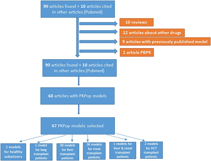
Sigma plot of the scientific literature review of population pharmacokinetic (PKPop) models for tacrolimus. PBPK, physiologically based pharmacokinetics

2.2. Meta‐model development

After literature review, the meta‐model was developed and validated both internally and externally. Individual‐level data (including in‐house and unpublished data and data received from some of the authors of published studies22, 23, 24, 25, 26) were used for model development, internal and external validation (Table 1), while summary‐level data were only used for external validation of the model. Individual‐level data are from paediatric and adult recipients of a kidney, liver, heart or lung at different times after transplantation.

Table 1.

Patient‐level databases available

Database	Adults/children	Organ transplanted	No of patients	No of observations	PK dosage (time after last dose, h)	Analytic method	Time after transplantation in days	Model‐building or external evaluation patients	Data source
1	Children	Liver	42	1344	C0	MEIA/CMIA	D1–D394	Model‐building	22
2	Children	Liver	15	166	0, 0.5, 0.75, 1, 2, 3, 4, 6, 8, 12	MEIA	D15	Model‐building	23
3	Children	Liver	82	1024	C0	MEIA	D1–D15	Model‐building	24
4	Adults	Kidney	65	423	0, 0.248, 0.64, 0.98, 1.37, 2.38, 11.03	MEIA	D15	Model‐building	25
5	Adults	Patient on waiting list for kidney transplantation	19	191	1, 2, 4, 8, 12	LC–MS/MS	‐	Model‐building	26
6	Adults	Liver	14	88	2, 4 C0, 1, 2, 4, 6, 8, 12	MEIA	D2 D8	Model‐building	In‐house
7	Adults	Liver	57	430	C0	MEIA	D1‐D8	Model‐building	In‐house
8	Adults	Lung	61	2471	C0, 0.33, 0.67, 1, 1.5, 2, 3, 4, 6, 8, 10, 12, 24	EMIT	D1–D459	External evaluation patients	Stimmugrep trial
9	Adults	Heart	20	548	C0, 0.33, 0.67, 1, 1.5, 2, 3, 4, 6, 8, 10, 12	LCMS	D8–D468	External evaluation patients	Pigrec trial
10	Adults	Kidney	32	1528	C0, 0.33, 0.66, 1, 1.5, 2, 3, 4, 6, 9, 12	LCMS	D6‐D208	External evaluation patients	PCCP trial

CMIA: chemiluminescent microparticle immunoassay; EMIT: enzyme multiplied immunoassay technique; LCMS: liquid chromatography‐mass spectrometry LC–MS/MS: liquid chromatography with tandem‐mass spectrometry; MEIA: microparticle enzyme immunoassay; PK, pharmacokinetic

2.2.1. Meta‐model building

Nonlinear mixed effects modelling was performed using NONMEM v7.3.0. (double precision, Icon Development Solutions, Ellicott City, MD, USA) and Perl‐speaks‐NONMEM (PsN)‐toolkit,27 a programming library containing a collection of computer intensive statistical methods for nonlinear mixed effects modelling, Xpose 4.0,28 and R software version 3.3.2.29 The first‐order conditional estimation method with interaction was used to model TAC PK.

• iStructural model

The following structural models were tested: 1‐ and 2‐compartment disposition models with first order elimination, 0 or first‐order absorption and with and without lag time and Erlang model of absorption. Time dependency was subsequently tested on absorption and on elimination. Assessment of model adequacy and decisions about increasing model complexity were driven by the data and guided by goodness‐of‐fit criteria, including (i) visual inspection of diagnostic scatter plots, (ii) successful convergence of the minimization routine, (iii) results of likelihood ratio tests, (iv) plausibility of parameter estimates, (v) precision of parameter estimates, and (vi) correlation between model parameter estimates <0.95.

• iiStochastic model

All interindividual error terms were described by an exponential error model or log‐normal parameter distribution (see equation 1).

$$P_i=\mathit{TVp}\times \exp \left({\eta }_i\right)$$ (1)

where: Pi is the estimated parameter value for individual i. TVp is the typical population value (geometric mean) of the parameter and η _i are individual‐specific interindividual random effects for individual i and parameter P and are assumed to be symmetrically distributed, zero‐mean random variables with a variance that is estimated as part of model fitting.

For PK observations in this analysis, the residual error model was initially described by a combined additive and proportional error model (see Equation 2):

$$Y=F\times \left(1+{\epsilon }_1\right)+{\epsilon }_2$$ (2)

where Y represents the observed concentration, F is the individual predicted concentration and ε₁ and ε₂ are the proportional and the additive error terms on TAC concentrations, respectively. ε'S were supposed to be symmetrically distributed, zero‐mean random variables with variance terms that are estimated as part of the population model‐fitting process.

• iiiCovariate model

Known physiological relationships such as effects of body size on TAC distribution and elimination were incorporated into the covariate–parameter models when permitted by available data. For example, the change in apparent clearance and volumes of distribution as functions of body weight was empirically described by an allometric model (see equation 3).

$$P_i=\mathit{TVp}\times {\left(\frac{{\mathit{WT}}_i}{{\mathit{WT}}_{\mathit{med}}}\right)}^{{\theta }_{\mathit{WT}}}$$ (3)

where P _i, the parameter value in individual i, was described as a function of typical PK parameter value (TVP) and of weight (WT) for individual i (WT _i), normalized by the median WT (WT_med). θ_WT is an estimated parameter describing the normalized power function.

The effects of categorical covariates were similarly assessed as shown in equation 4.

$$P_i=\mathit{TVp}\times {\left({\theta }_{\mathit{COV}}\right)}^{\mathit{COV}}$$ (4)

where P _i is the parameter value for an individual patient, TV_P is the reference parameter value, θ_COV is the parameter characterizing the covariate effect and COV is the covariate value in the dataset, which was coded as 0 or 1 for binary categorical variables.

A covariate modelling approach emphasizing parameter estimation rather than stepwise hypothesis testing was implemented for this population PK analysis. First, predefined covariate–parameter relationships were identified based on exploratory graphics, scientific interest, mechanistic plausibility of prior knowledge, and a full model was constructed with care to avoid correlation or collinearity in predictors (covariates with correlation coefficients >0.6 were not simultaneously included as potential predictors). Inferences about clinical relevance of parameters were based on the resulting parameter estimates of the full model and measures of estimation precision (asymptotic standard errors, bootstrap 95% confidence intervals or log‐likelihood profile).

Covariates tested on apparent volumes of distribution and clearance included: body weight, age, type of transplantation and time after transplantation.

2.2.2. Meta‐model internal evaluation

In addition to plausibility of estimated parameter, standard methods as described by Owen and Fiedler‐Kelly30 were used for internal validation of the model. They include diagnosis scatter plots, prediction‐corrected visual predictive checks (pcVPCs) and the bootstrap.

Diagnosis scatter plots, also called goodness‐of‐fit plots, consist in a series of graphs, such as observed concentrations vs predicted concentrations and normalized prediction distribution errors and conditional weighted residuals vs time.

To generate the pcVPC, the original data set is simulated many times using the final model. The 90% prediction interval of the simulated concentration time profiles should cover 90% of the observed concentrations. A good overlapping between predicted and observed drug concentrations enables to conclude that the model is adequately adjusted to data. One thousand simulation replicates of the original data set were generated using the final model. Overlay plots of the observed concentrations vs time with the 95% prediction interval of the simulated data were generated.

Bootstrapping consists in generating a large number of new databases by sampling individuals with replacement from the original dataset. For each new dataset, parameters were re‐estimated and this resulted in a bootstrap distribution of each model parameter. Empirical 95% confidence intervals (CI) were constructed by observing the 5th and 95th percentiles of the resulting parameter distributions for those bootstrap runs that generated parameter estimates.

2.2.3. Meta‐model external evaluation

External evaluation was performed in 2 different ways: (1) available patient‐level data (observed concentrations from studies not included in the model building dataset) were predicted using the final model with MAXEVAL = 0 option in NONMEM. The good predictive performance of the model is established if the model predictions are consistent with observed data; (2) comparing parameter estimates from the final meta‐model to the ranges of parameters from the previously published models.

The individual‐ (patient‐) level data were originated from 3 multicentre PK trials intended to develop population PK models and Bayesian estimators for optimized dose adjustment of immunosuppressive drugs in thoracic and renal transplant patients. The design characteristics of the 3 studies are summarized in Table 1.

2.3. Nomenclature of targets and ligands

Key protein targets and ligands in this article are hyperlinked to corresponding entries in http://www.guidetopharmacology.org, the common portal for data from the IUPHAR/BPS Guide to PHARMACOLOGY.31

3. RESULTS

Figure 1 and Table 2 represent the PRISMA flow diagram describing the different steps for study selection and the summary table including details of the studies retained from the literature review exercise, respectively. A total of 109 publications were initially generated by PubMed search. Among these, 42 were excluded in accordance with the exclusion criteria. To the 67 selected articles, nine additional studies were added from reference scanning. A total of 76 articles were retained, in which 76 developed models were found to be relevant for meta‐model building and the related parameters recorded (see Table 2).

Table 2.

Published tacrolimus pharmacokinetic population models (results of systematic review)

Organ transplanted, No. of patients	Type of population	Pharmacokinetic model	Pharmacokinetic parameters	Model variability	References
Kidney 70	Adults	1‐CMT model with first‐order absorption	Dosage with ELISA: CL/F = 31.3 V/F = 854 T½ = 22.2 * Dosage with LC–MS/MS: CL/F = 33.5 L/h V/F = 898 L T ½ =18.6 h	* dosage with ELISA: IIV CL/F = 47% IIV V/F = 247% AddRE = 4.1 ng/mL * dosage with LC–MS/MS: IIV CL/F = 42% IIV V/F = 111% AddRE = 3.7 ng/mL	Staatz et al.32
Kidney 70	Adults	1‐CMT model with first‐order absorption And elimination	CL/F = 23.6+(31.9/DOT)+(76.7/AST) V/F = 1070 Ka = 4.48 (fixed)	IIV CL/F = 42% IIV V/F = 111 L AddRE = 3.7 ng/mL	Staatz et al.33
Kidney 43	Adults	2‐CMT model with first‐order absorption with a lag time	F = 0.23 (fixed) Tlag = 0.956 Ka = 0.58 Ke = 0.517 V1 = 0.18 L/kg K12 = 2.85 K21 = 0.384	NA	Scholten et al.34
Kidney 83	Adults	1‐CMT model with first‐order absorption and elimination	CL = 1.81 × [1+(POD2.54/(POD2.54+3.812.54))] × (1.575, if concomitant prednisone > 25mg) Vd = 98.4 F = 0.137 Ka = 4.5 (fixed)	IIV CL =31% IIV V = 79% IIV F = 32% AddRE = 0.96 ng/mL PropRE = 18.6%	Antignac et al.35
Kidney 31	Adults	2‐CMT model With first‐order absorption and first‐order elimination	F = 0.23 × [1 − (DD/(25+DD))] × (0.85 if prednisolone < 10mg) Ka = 3.7 (once‐daily dosing) Ka = 1.6 (twice‐daily dosing) CL = 3.7 (CYP3A5*3/*3) CL = 5.5 (CYP3A5*1/*3) Vc = 61 (once‐daily dosing) Vc = 42 (twice‐daily dosing) Q = 10 Vp = Vc	IIV CL = 19% IIV Vc = 28% IOV F = 22% PropRE = 23%	Press et al.36
Kidney 32	Adults	2‐CMT model, 3 transit absorption CMTs	CL/F = 863/HCT HCT (%) = 28.6 [21–39] CL/F range with/without HCT were 3–128 L/h and 6–77 L/h, Ktr = 6.5 Vc/F = 147 Vp/F = 500 (fixed) Q/F = 60	IIV Ktr = 15% IIV Vc/F 26% IIV CL/F = 30% IIV Q/F = 63% IOV Ktr = 24% IOV Vc/F = 71% IOV CL/F = 27% PropRE = 10% AddRE = 0.7 ng/mL	Benkali et al.37
Kidney 19	Adults	2‐CMT model with first‐order absorption.	Ka = 2.18 Ka = 2.02 (night) Vc/F = 142 Vp/F = 192 Q = 43 CL = 22+34CYP3A5+10ABCB1 CYP3A5 = 1 if CYP3A5 *1 carriers, otherwise CYP3A5 = 0 ABCB1: Not clear how it was categorized.	IIV CL/F = 6% IIV V1/F = 33% IIV V2/F = 192% AddRE =0,02 ng/mL PropRE = 29% PropREMEIA = 22%	Musuamba et al.26
Kidney 12	Adults	1‐CMT model with double γ absorption and first‐order elimination	C0 = 0.816 ± 0.441 a1 = 13.358 ± 6.182 b1 = 20.414 ± 6.564 a2 = 7.397 ± 1.581 b2 = 2.183 ± 0.273 r = 0.684 ± 0.146 F*A_IV = 1.846 ± 1.359 a = 0.199 ± 0.178 Mean values (± SD) on day 14 post‐transplant; a1, b1, a2 and b2 are the parameters of the γ distribution, r is the fraction of drug absorbed through the first route, F is the bioavailability, A_IV is the initial concentration; α is the apparent elimination rate after intravenous bolus administration of a unit dose, C0 is the trough concentration.	NA	Saint Marcoux et al.38
Kidney 46 building, 17 validation	Adults	1‐CMT model with first‐order absorption	Ka = 4.5 (fixed) CL = 0.862+(0.32 × DD)+(1.16 if concomitant prednisolone > 25mg) V = 1661 L F = 1.18	Prop RE = 31.0%	Velickovic‐Radovanovic et al.39
Kidney 41	Adults	2‐CMT model, 3 transit absorption CMTs	CL/F = 19,if CYP3A5*3/*3 or = 40.85,if CYP3A5*1/*1 & CYP3A5*1/*3 Vc/F = 486 Ktr = 3.3 K12 = 0.73 K21 = 0.09	IIV Ktr = 52% IIV Vc/F = 53% IIV CL/F = 35% IIV k12 = 54% PropRE = 8% AddRE = 0.7 ng/mL	Benkali et al.40
Kidney 73	Adults	2‐CMT model with Erlang absorption (n = 3) and first‐order elimination	Ktr1 = 3.34 × (1.53 if Prograf®) CL/F = 21.2 × (HCT/35)−1.14 × (2 if CYP3A5 expressers) Q/F = 79 Vc/F = 486 × (0.29 if Prograf®) Vp/F = 271	IIV Ktr = 24% IIV CL/F = 28% IIV Q/F = 54% IIV Vc/F = 31% IIV Vp/F = 60% PropRE = 14.9%	Woillard et al.41
Kidney 45	Adults	1‐CMT model with γ absorption, with 2 parallel absorption routes, and first‐order elimination	CL/F = 26.3 ± 12.2 L/h (LC–MS/MS) # CL/F = 23.4 ± 12.1 L/h (CMIA)# CL/F = 23.4 ± 12.1 L/h (EMIT)# Vd/F = 405 ± 171 L (LC–MS/MS)#,§ Vd/F = 321 ± 168 L (CMIA)c Vd/F = 264 ± 125 L (EMIT)#,§ #mean values (±SD) § variance of log transformed parameter (approximately equal to the coefficient of variation squared), unitless	NA	Saint Marcoux et al.42
Kidney 681	Adults	NR	CL/F = 38.4 × [(0.86, if POD 6 − 10)or(0.71, POD 11 − 180) ] × [(1.69, if CYP3A5 * 1/ * 3 )or(2.00, if CYP3A5 * 1/ * 1 )] × (0.70, if receiving a transplant at a steroid sparing center) × [(AGE/50)−0.4] × (0.94, if CCB is present)	IIV CL/F = 40.1% AddRE = 3.19	Passey et al.43
Kidney 70	Adults	2‐CMT model with first‐order elimination, first‐order absorption with lag time	$\frac{\mathit{CL}}{F}=16.3+\left(20.6\times \mathit{HCT}/21\right)+\left(15.4,\text{if}\mathrm{CYP}3\mathrm{A}5*1\right)+\left(7.6,\text{ifABCB}11236\mathrm{CC},2677\mathrm{GG}\text{and}3435\mathrm{CC}\right)\text{ka}=0.45/h$ Vc/F = 86.4 Vp/F = 1115 Q/F = 58.2 Tlag = 0.1	IIV Ka = 91% IIV Vc = 55% IIV Vp = 48% IIV CL = 32% IIV Tlag = 61% PropRE = 13% AddRE = 0.88 ng/mL	Musuamba et al.25
Kidney 80	Adults	1‐CMT model with first‐order absorption and elimination	$CL\mathit{/}F\mathit{=}\mathit{22}\mathit{.}\mathit{9}\mathit{\times }exp\left[\left[\mathit{0}\mathit{.2225},\mathit{\text{if}}CYP\mathit{3}A{\mathit{5}}^{\mathit{*}}\mathit{1}{\mathit{/}}^{\mathit{*}}\mathit{1}\right]\mathit{\text{or}}\left[\mathit{0}\mathit{.}\mathit{17},\mathit{\text{if}}CYP\mathit{3}A{\mathit{5}}^{\mathit{*}}\mathit{1}{\mathit{/}}^{\mathit{*}}\mathit{3}\right]\mathit{\text{or}}\left[\mathit{0}\mathit{.}\mathit{0525},\mathit{\text{if}}CYP\mathit{3}A{\mathit{5}}^{\mathit{*}}\mathit{3}{\mathit{/}}^{\mathit{*}}\mathit{3}\right]\right]\times \mathit{exp}\left[\left[0.297,\mathit{\text{if}}\mathit{HCT}\le 33\right]\mathit{\text{or}}\left[0.117,\mathit{\text{if}}\mathit{HCT}>33\right]\right]\times {\mathit{POD}}^{-0.00762}$ V/F = 716 × exp(0.355 × WT/59.025) Ka = 4.5 (fixed)	IIV CL/F = 49.8% IIV V/F = 48.7% PropRE = 40%	Han et al.44
Kidney 65 generated from 4 previous models	Adults	2‐CMT model with first‐order absorption with a lag time and first‐order elimination	Ka = 1.68 Tlag = 0.045 CL/F = 3.85 Vc/F = 221 Vp/F = 521 Q/F = 21.9	IIV Ka = 199% IIV Tlag = 350% IIV CL/F = 185% IIV V1/F = 133% IIV V2/F = 144% AddRE = 0.97 ng/mL PropRE = 1%	Musuamba et al.45
Kidney 161	Adults	1‐CMT model with first‐order absorption and elimination	V/F = 1020 Ka = 3.09 CL/F = 26.6 × (HCT/27.9)−0.45 × (1.21 if CYP3A5 * 1/ * 1 or CYP3A5 * 1/ * 3, CYP3A4 * 1/ * 1G) × (0.982 if CYP3A5 * 1/ * 1 or CYP3A5 * 1/ * 3, CYP3A4 * 1/ * 1) × (0.77 if CYP3A5 * 3/ * 3, CYP3A4 * 1/ * 1G or CYP3A4 * 1G/ * 1G) × (0.577 if CYP3A5 * 3/ * 3, CYP3A4 * 1/ * 1) Vd/F = 1090	IIV CL/F = 44.2% V/F = 56.6% AddRE = 1.47 ng/mL PropRE = 19.8%	Zuo et al.46
Kidney 102	Adults	2‐CMT model with first‐order absorption with lag time	CL/F = 20.7 × (AGE/50)−0.78 × (2.03 if CYP3A5 expressers) × (1.40 if MRP2 genotype H2/H2 or H1/H2) Vc/F = 234 Vp/F = 1319 Q/F = 70.7 Ka = 0.544 Tlag = 0.183 × (2.60 for patient with diabetes)	IIV CL/F = 43.9% IIV Vc/F = 157% PropRE = 18.4%	Ogasawara et al.47
Kidney 99	Adults	3‐CMT nonparametric model with first‐order absorption and a lag time	CL/FCYP=26.7 CL/FnoCYP=21.2 Q/F = 19.5 Vc/F = 177 Vp/F = 3707 Tlag1 = 1.00 (POD = first week) Tlag2 = 0.15 (POD = week 2–4) Tlag3 = 0.59 (POD > 1 month)	NA	Åsberg et al.48
Kidney 69	Adults	2‐CMT model, first‐order absorption with a lag time	CL/Fn = 20.5 × (FFM/60)0.75 Vc/Fn = 107 × (FFM/60) Q/Fn = 37.3 × (FFM/60)0.75 Vp/Fn = 424 × (FFM/60) Ka = 1.14 Ka (study 2) = 0.37 Tlag = 0.22 Tlag (study 2) = 0.81 F = [2.04+(1 − 2.04)/(1+(POD/2.5)−9.4)] × [1+0.28/(1+(POD/31)−2.5)] × [Fminage+(1 − Fminage)/(1+(AGE/47)−14)] × 0.51 if CYP3A5 expressers Fminage = 0.43 in females and 0.66 in males; Fn, bioavailability at baseline nadir (5 days after transplantation)	IIV CL/Fn = 33% IIV Vc/Fn = 14% IIV Q/Fn = 91% IIV Vp/Fn = 52% IIV HillFlate = 117% R (CL/Fn, Q/Fn) = 0.75 IOV Fn = 16% IOV Ka = 63% PropRE = 16.7% Factor for residual variability: Study 2: 0.57 Study 3: 0.73	Storset et al.49
Kidney 173	Adults	2‐CMT model with first‐order absorption with a lag time	CL/F = 25.5 × (1.6, if CYP3A5 expressers) × [1+(−1.01 × (HCT − 0.33))] × (WT/70)0.75 × [1+(−0.0021 × (POD − 22.7))] Vc/F = 113 × [1+(−0.0028 × (PRED − 155.5))] Q/F = 67.9 Vp/F = 1060 Ka = 0.35 Tlag = 0.44 PRED = Cmax value of free prednisolone (nmol/L)	IIV CL/F = 29.5% IIV Vc/F = 46.8% IIV Vp/F = 89.4% IIV Ka = 47.6% IOV CL/F = 29.9% IOV Vc/F = 126.5% Corr R (Vc/F, ka) =67.7% R (Vc/F, Vp/F) = −4.9% R (Ka, Vp/F) = −1.3% PropRE = 18.3%	Bergmann et al.50
Kidney 105	Adults	1‐CMT model with first‐order absorption	CL/F = 10.017 × (POD/47)−0.0283 × (WT/68)0.869 × (TP/63)0.161 × [1 − (0.086 × (AST − 15))] × [1 − (0.831 × (HCT − 0.31))] V/F = 0.68 (fixed) Ka = 1.3 (fixed)	IIV CL =15.2 L/h AddRE = 4.066 ng/mL	Golubovic et al.51
Kidney 122	Adults	1‐CMT model with first‐order absorption	CL/F = 21.9 × [1+0.0119 × (POD − 9.6)] × (0.816, ifCYP3A5 * 3/3 )CYP Ka = 3.43 Tlag = 0.25 (fixed) V/F = 205	IIV CL/F = 42.6% IIV V/F = 64.6% IIV Ka = 158.9% PropRE = 5.4% AddRE = 1.94 ng/mL	Han et al.52
Kidney 242	Adults	2‐CMT model with first‐order absorption and a lag time	Ka = 1.01 Tlag = 0.41 Model: (estimate for a typical patient with HCT 45%, FFM 60 kg, CLwb/F = 16.1, Vcwb/F = 125 L, Qwb/F = 23.8, Vpwb/F = 636 L) Plasma CL/F = 811 × (FFM/60)0.75 × 1.30 (If CYP3A5 expresser) Plasma Vc/F = 6290 × FFM/60 Plasma Q/F = 1200 × (FFM/60)0.75 Plasma Vp/F = 32100 × FFM/60 F = 1 × [1 – (0.67 × Prednisolone dose)/(35 mg+Prednisolone dose)] × 2.68 (If first day post − transplant) × 0.82 (If CYP3A5 expresser)	IIV CLwb/F = 40% IIV Vc/F = 54% IIV Qwb/F = 63% IIV Fday2 = 57% R (CLwb/F, Vcwb/F) = 0.43 R (CLwb/F, Qwb/F) = 0.62 IOV F = 23% IOV Ka = 120% PropRE = 14.9%	Storset et al.53
Kidney 16	Adults	2‐CMT model, with 3 transit absorption CMTs	CL = 16.50 L/h Vc = 9.89 L Q = 35.56 L/h Vp = 526.03 L Ka = 0.47/h MT = 0.83 h Ktr = 3.61/h MT: (mean transit time)	IIV CL = 39% IOV CL = 29% IIV Ka = 35% IIV MT = 32% PropRE = 21%	Andreu et al.54
Kidney 83	Adults	1‐CMT model with first‐order absorption	CL/F = 23.3 × [(1.04 × Gene1)+(0.83 × Gene2)+(0.62 × Gene 3)] Vd/F = 204 (fixed) Gene1 = 1 if patient is CYP3A5*1 carrier and POR*28CC or CT, otherwise = 0 Gene2 = 1 if patient is CYP3A5*1 carrier but not POR*28CC or CT, otherwise = 0 Gene3 = 1 if patient is not CYP3A5*1 carrier, otherwise = 0	IIV CL/F = 26.3% IIV V/F = 10% fixed ExRE = 21.1% AddRE = 0.81 ng/mL	Zhang et al.55
Kidney 96	Adults	1‐CMT model with first‐order absorption	CL/F = 21.5 × e−0.05 × (HB − 11.8) × (−0.06)(DOT/125) V/F = 333 Ka = 7.06 fixed	IIV CL/F = 36.8% IIV V/F = 63.64% AddRE = 0.88 ng/mL PropRE = 23.17%	Vadcharavivad et al.12
Kidney 70	Adults	2‐CMT model with first‐order elimination, first‐order absorption with lag time	Tlag = 0.47 h Ka = 0.23/h CL/F = 35 × [1+(0.45, if CYP3A5 expressers) or (0.41, if CYP3A5 missing)] × (WT/70)0.75 × (γGT/13)−0.21 × (HCT/0.34)−0.59 Vc/F = 12 × (WT/70) Q/F = 68 × (WT/70)0.75 Vp/F = 109 × (WT/70)	IIV Ka = 58% IIV CL/F = 45% IIV V1/F = 170% IOV CL/F = 25% PropRE = 21%	Prytula et al.56
Kidney 83	Adults	1‐CMT model with first‐order absorption	CL/F = 22.4 × exp(−0.0526 × (83/POD)) × (39.1/HCT)0.548 × exp(−0.32 × CYP3A5) V/F = 179 × POD0.842 Ka = 4.5 fix	IIV CL/F = 50,0% IIV V/F = 60.4% AddRE = 2.33 ng/mL	Zhang et al.57
Kidney 59	Adults	1‐CMT model with double γ absorption route	C(t) = C(t)TPV × (0.77)CYP3A C0 = 2.94 a1 = 12.33 b1 = 20.36 a2 = 15.19 b2 = 5.05 r = 0.46 F*AIV = 24.52 Α = 1.52		Woillard et al.58, a
Kidney 304	Adults	2‐CMT model with first‐order absorption and a lag time	CL = 20.5 if CYP3A4*1/*1 homozygotes with at least 1 active CYP3A5*1 allele CL = 12.5 if CYP3A4*22 noncarriers with CYP3A5*3/*3 or CYP3A4*22 carriers with CYP3A5*1/*1 CL = 9.1 if CYP3A4*22 carriers with CYP3A5*3/*3 CL_AGE = −0.205 CL_AGE: The change on clearance for patients aged ≥63 years Q = 4.2 Vc = 5.02 Vp = 526 (fixed) Ka = 0.138 Tlag = 0.243	IIV CL = 27.8% IOV CL = 33.3% PropRE = 25%	Andreu et al.59
Liver 57 Kidney 49	Adults	1‐CMT model with first‐order elimination, double γ absorption	Kidney transplant patient, ITSIM: FAIV: 2.8 (μg/L) a1 = 7.9 b1 = 5.6 (/h) a2 = 13.8 b2 = 2.3 (/h) r = 0.4 α = 0.17/h Cmax = 12.1 μg/L Tmax = 6.3 h Kidney transplant patient, Pmetrics: FAIV: 2.3 (μg/L) a1 = 19.4 b1 = 5.9 (/h) a2 = 20.7 b2 = 6.8 (/h) r = 0.6 α = 0.15/h Cmax = 1241 μg/L Tmax = 5.4 h Liver transplant patient, ITSIM: FAIV: 2.6 (μg/L) a1 = 5.2 b1 = 5.5 (/h) a2 = 14.3 b2 = 2.9 (/h) r = 0.21 α = 0.18/h Cmax = 11.7 μg/L Tmax = 5.5 h Liver transplant patient, Pmetrics: FAIV: 2.0 (μg/L) a1 = 27.2 b1 = 5.5 (/h) a2 = 20.8 b2 = 8.6 (/h) r = 0.62 α = 0.18/h Cmax = 12.5 μg/L Tmax = 5.6 h		Woillard et al.60
Kidney 67	Adults	2‐CMT model with first‐order absorption and elimination and an absorption lag time	CL/F = 19.7 × (1.45, if CYP3A5 * 3 * 6 * 7 intermediate metabolizer) × (2.25, if CYP3A5 * 3 * 6 * 7 extensive metabolizer) Vc/F = 234 × (WT/85.9) Vp/F = 403 Q/F = 52.6 Ka = 4.21 Tlag = 0.828	IIV CL/F = 37% IIV Vc/F = 76.7% IIV Q/F = 48.6% IIV Ka = 69.4% PropRE = 9.00	Campagne et al.61
Kidney 50	Paediatrics	2‐CMT model, first‐order absorption with lag time	Tlag = 0.356 h Ka = 0.462/h V1/F = 57.9 × (WT/70) V2/F = 566 × (WT/70) Q/F = 79.7 × (WT/70)0.75 CL/F = 13.9 × (WT/70)0.75 × 2.26CYP3A5 + 7.11 × 79.7HCT CYP3A5 = 0 if patient is an CYP3A5 nonexpresser, otherwise = 1; HCT = 0 if HHT level is ≥0.33, otherwise = 1.	AddRE = 3.2 IIV Ka = 76.2% IIV Q/F = 89.9% IIV V1/F = 132% IIV CL/F = 41.9%	Zhao et al.62
Kidney 22	Paediatrics	1‐CMT model with first‐order absorption and lag time	Tlag = 0.872 h Ka = 8.34/h V/F = 1100 × (WT/70) L CL/F = 30.6 × (WT/70)0.75 × 1.66CYP3A5 CYP3A5 = 1 if CYP3A5 *1/*3 CYP3A5 = 0 if CYP3A5*3/*3	IIV Ka =150% IIV V/F = 52.1% IIV CL/F = 34.6% ExER = 22.1%	Zhao et al.63
Kidney 53	Paediatrics	2‐CMT model with first‐order input with lag time	$\mathit{Ka}=0.52\times \left[\begin{array}{c}1+\left(-0.76\text{if patient is}\mathrm{on}{\mathit{\text{Limustin}}}^{\circledR }\right)\mathit{\text{or}}\\ \left(-0.51\text{for unknown formulation}\right)\end{array}\right]$ $F=100\times e^{-0.3\times \left(\mathit{DD}-2\right)}\times \left[\begin{array}{c}1+\left(-0.53\text{if patient is}\mathrm{on}{\mathit{\text{Limustin}}}^{\circledR }\right)\mathit{\text{or}}\\ \left(-0.53\text{for unknown formulation}\right)\end{array}\right]$ $\mathit{CL}/F=11.98\times \left[\begin{array}{c}1+\left(0.5\text{for}\mathrm{CYP}3\mathrm{A}5*1/*3\right)\mathit{\text{or}}\\ \left(0.93\text{for}\mathrm{CYP}3\mathrm{A}5*1/*1\right)\end{array}\right]$ Vc/F = 24.16 Q/F = 32.49 L/h Vp/F = 383.5 Tlag = 0.39	IIV Ka = 37% IIV Vc/F = 66% IIV F = 38% IIV RE =35% AddRE = 0.12 [ln (ng/mL)]	Jacobo‐Cabral et al.64
Kidney 69	Paediatrics	2‐CMT model	$\mathit{CL}/F=50.5\times {\left(\mathit{WT}/70\right)}^{0.75}\times \left[\begin{array}{c}\left(1.0,\text{if}\mathrm{CYP}3\mathrm{A}5*3/*3\text{or unkown}\right)\\ \text{or}\left(2.0,\text{if}\mathrm{CYP}3\mathrm{A}5*1/*3\text{or}\mathrm{CYP}3\mathrm{A}5*1/*1\right)\end{array}\right]\times \left(0.74,\text{if living donor}\right)\times {\left(\mathit{\text{eGFR}}/69\right)}^{0.19}\times \left[{\left(\mathit{HCT}/0.3\right)}^{-0.44},\text{if}\mathrm{HCT}<0.3\right]$ Vc/F = 206 Vp/F = 1520 Q/F = 114 Ka = 0.56 Tlag = 0.37	IIV Ka = 188% IIV CL/F = 25% IIV Vc/F = 69% IIV Vp/F = 62% IOV CL/F = 18% IOV Vp/F = 35% AddRE IA =1.01 AddRE LC–MS/MS = 0.28 PropRE IA = 0.13 PropRE LC–MS/MS =0.21	Andrews et al.65
Liver 40	Adults	1‐CMT model with first‐order absorption and first‐order elimination	F = 0.25 (fixed) Ka = 0.45/h Ke = 0.05 (POD 1–4 days), 0.05 (POD 5–7 days), 0.03 (POD 8–11 days), 0.07 (POD 12–14 days)/h V = 0.62 (POD 1–4 days), 0.98 (POD 5–7 days), 2.66 (POD 8–11 days), 1.43 (POD 12–14 days) L/kg	NA	Macchi‐Andanson et al.66
Liver 35	Adults	1‐CMT model	CL = [0.737+(0.0134 × POD)] × 0.728HF × 0.809RF × HW/600 HF = 1 if total bilirubin concentration > 2.5 mg/dL, otherwise = 0. RF = 1 if serum creatinine concentration > 1 mg/dL, otherwise 0 V = 1.52 L/kg F = 0.067	IIV CL = 57.4% IIV V = 39.7% IIV F = 63.0% r (CL,F) = 0.776 AddRE = 2.9 ng/mL	Fukatsu et al.67
Liver 68	Adults	1‐CMT model with first‐order absorption	CL/F = 29.6 (AST < 70) CL/F = 24.0 (AST > 70) Vd/F = 601 × (WT/72.1) Ka = 4.48 (fixed)	IIV CL/F = 43% IIV V/F = 93% AddRE = 3.3 ng/mL	Staatz et al.68
Liver 47	Adults	1‐CMT model	CL = (0.743+(0.0157 × POD)) × 0.792HF × 0.810RF × HW/600 V = 1.64 × BW F = 0.0732 BW = bodyweight; HF = 1 if total bilirubin >2.5 mg/dL; otherwise = 0.; HW = hepatic weight; RF = 1 if serum creatinine >1 mg/dL, otherwise = 0.	IIV F = 71.2% IIV CL = 60.0% IIV V = 35.4% R (CL/F) = 0.770 AddRE = 2.75 μg/L	Fukudo et al.69
Liver 37	Adults	1‐CMT Model with first‐order absorption	$\mathit{CL}/F=\left(\mathit{CL}/F_{\mathit{max}}\times {\mathit{POD}}^{4.9}\right)/\left({\mathit{TCL}}_{50}^{4.9}+{\mathit{POD}}^{4.9}\right)$ CL/Fmax = 36 × (ALB/38)0.64 TCL50 = 6.3 × (ASAT/38)0.28 V/F = 1870 Ka = 4.48 (fixed) TCL50 is the time needed to obtain 50% of maximum CL/F	IIV CL/Fmax = 43.6% IIV TCL50 = 33.2% IIV V/F = 49% r (CL/Fmax,Vd/F) = 0.55 AddRE = 3.07 ng/mL	Antignac et al.70
Liver 67	Adults	1‐CMT model with first‐order absorption	CL/F = 21.3+(9.83 × (1 − HCT))+(3.43 × (1 − ALB))+(22.13 × (1 − DIL))+( 27.43 × (1 − FLU)) V/F = 314.0 Ka = 4.5 (fixed)	IIV CL/F = 31.6% PropRE = 24.3%	Zahir et al.71
Liver 29	Paediatrics and adults	1‐CMT model with first‐order absorption	Model 1, according for blood concentration: CL/F = 14.1+( 0.237 × (WT − 55))+(−2.93)ALP+(−0.0801 × (SCR − 60)) V/F = 217+(−7.83 × (HCT − 31.1))+(179 × (HT − 1.61)) Ka = 2.08 With ALP = 1 if alkaline phosphatase ≥ 200 U/L, otherwise 0. SCR = serum creatinine Model 2, according for plasma concentration: CL/F = 537+( 10.5 × (WT − 55)) V/F = 563+5380CECP CECP = 1 if erythrocyte to plasma ratio of concentration ≥ 68, otherwise = 0.	Model 1: IIV CL/F = 65.7% IIV V/F = 63.8% PropRE = 34.8% Model 2: IIV CL/F = 96.0% IIV Vd/F = 105.4% AddRE = 0.548 ng/mL	Sam et al.72
Liver 72	Adults	1‐CMT model with first‐order absorption and elimination	CL/F = 15.9 − (1.88 × TBIL)+(7.65 × CYPD)+(7.00 × CYPR) V/F = 620 Ka = 4.48 (fixed) If total biblirubin ≤25.7, μmol/L, TBIL = 0, if biblirubin = 25.8–51.4, TBIL =1,, if biblirubin = 51.5–77.1, TBIL = 2, if biblirubin = 77.2–128.5, TBIL = 3, if biblirubin >128.5, TBIL = 4 CYPD: Donor CYP3A5*3/ *3 = 0; others = 1 CYPR: Recipient CYP3A5*3/ *3 = 0; others = 1	Model 2: IIV CL/F = 31.2% IIV V/F = 55.0% AddRE = 2.81 ng/mL	Li et al.73
Liver 14	Adults	2‐CMT model with first‐order absorption and first‐order elimination. Hill model to describe the relationship between AUC12effCNA and TAC AUC12	Ka = 4.03/h CL/F = 2.85 × 0.36W/S × 1.026FV Q/F = 22 L/h V1/F = 87 L V2/F = 1290 L AUC12effCNA = Min + Delta × (1 – (AUC12 S/((AUC12)50 S+ AUC12 S) This Hill model describe the relationship between tacrolimus exposure (AUC12Tacrolimus) and the area under the calcineurin activity (CNA)‐time curve over 12 hours (AUC12effCNA) Min = 99 pmol/min/106 PBMC Delta = 3187 pmol/min/106 PBMC (AUC12)50 = 164 h.mg/mL Where W/S = whole/split cadaveric liver and FV: coagulation factor V, were expressed as 0 or 1a	IIV ka = 0.44 IIV CL/F = 0.23§ IIV V1/F = 0.44§ IIV Q/F = 0.39§ IIV V2/F = 0.36§ IIV Min = 0.16§ IIV Delta = 0.10§ IIV (AUC12)50 = 0.076§ IIV s = 0.12d IOV ka = 13.1d IOV CL/F = 0.30d IOV V1/F = 0.74d IOV Q/F = 0.85d IOV V2/F = 1.35d IOV Min = 0.093d IOV Delta = 0.064d IOV (AUC12)50 = 0.051d IOV s = 0.15d PropRE = 0.012 g	Blanchet et al.74
Liver 35	Adults	1‐CMT model with first‐order elimination	CL/F = (0.36+(2.01/POD) × L) × TBIL−0.23 × (0.49, if POD ≤ 3) × (0.75, if INR > 1.4) × (0.86, if GRWR ≤ 1.25%) × WT V/F = 568 TBIL = 1 if total bilirubin level ≤ 1.2 mg/dL, otherwise TBIL = total bilirubin level) L = 1 if POD >35 days, otherwise L = 0:	IIV CL/F = 35.35% IIV V/F = 68.12% AddRE = 3.14 ng/mL	Lee et al.75
Liver 262	Adults	1‐CMT model with first‐order administration, first‐order elimination	CL/F = 20.9 × (DDS/4)0.582 × (HCT/35.4)0.418 × (TP/69.1)0.780 × 0.841SU V/F = 808 × (HCT/35.4)1.52 × (TP/69.1)1.81	IIV CL/F = 23.8% IIV V/F = 70.4% ExpRE = 33.6% AddRE = 0.96 ng/mL	Zhang et al.76
Liver 75	Adults	1‐CMT model with first‐order absorption and first‐order elimination	Ka = 4.48 (fixed) CL/F (POD: 0–3 days) = 11.1 L/h, if AST < 500 U/L and rapid recovery CL/F (POD: 0–3 days) = 8.04 L/h for standard group Vd/F (POD: 0–3 days) = 328 L CL/F (POD: 4–15 days) = 24.5 L/h, if ALB <28% and HCT < 2.5 g/dL CL/F (POD: 4–15 days) = 17.8 L/h for standard group. Vd/F (POD: 4–15 days) = 568 L	IIV CL/F (POD: 0–3 days) = 45.9% IIV Vd/F (POD: 0–3 days) = 52.2% IIV CL/F (POD: 4–15 days) = 36.7% IIV Vd/F (POD: 4–15 days) = 20.2%	Oteo et al.77
Liver 150	Adults	1‐CMT model with first‐order absorption	Ka = 4.48 (fixed) CL/F (POD: 0–3 days) = 14.5 L/h CL/F (POD: 0–3 days) = 10.1 L/h (high AST) Vd/F (POD: 0–3 days) = 365 L CL/F (POD: 4–15 days) = 19.3 L/h CL/F (POD: 4–15 days) = 23.8 L/h (low HCT/albumin) Vd/F (POD: 4–15 days) = 597 L	AddRE = 3.04 ng/mL	Valdivieso et al.78
Liver 47	Adults	2‐CMT model with first‐order absorption	CL/F = 11.2 × Dose0.371 × POD0.127 Vc/F = 406 L Q/F = 57.2 L/h Vp/F = 503 L Ka = 0.723/h	IIV CL/F = 16.2% IIV Vc/F = 163% IIV Q/F = 19.7% IIV Vp/F = 199% IIV Ka = 74.3% PropRE = 26.54%	Zhu et al.79
Liver 112 healthy volunteers 40	Adults	2‐CMT model with first‐order absorption with lag time	CL/F = 32.8 for healthy volunteers CL/F = 32.8 × 0.562[exp((ALT/40) × 0.0237)] for transplant recipients Vc/F = 22.7 Vp/F = 916 (fixed) Q/F = 76.3 Ka = 0.419 (fixed) Tlag = 0.404	IIV CL = 46.6% IIV Vc = 57.3% IIV Q = 46.0% IIV Vp = 93.5% IIV Ka = 0%* PropRE = 39.8%	Lu et al.80
Liver 95	Adults	1‐CMT model with first‐order absorption	Ka = 4.48 (fixed) CL/F = 17.6 θPOD‐ CL/F = 0.205 θBUN‐ CL/F = − 0.116 θALP‐ CL/F = 0.165 θTBIL‐ CL/F = − 0.142 θHCT‐ CL/F = − 0.789 θCYP‐ CL/F = 0.661 V/F = 225 θPOD‐V/F = 0.852 θHB‐V/F = − 0.813	IIV CL/F = 53.9% IIV V/F = 68.0% PropRE = 28.4% AddRE =0.606 ng/mL	Zhu et al.81
Liver 29	Adults	1‐CMT model, with first‐order absorption	Ka = 0.52/d CL/F = 6.18 L/d V/F = 101 L CL/F and V/F: In the present of 3 direct‐acting antiviral regimen (3D) of ombitasvir, paritaprevir/ritonavir, and dasabuvir	IIV CL/F = 39% IIV V/F = 76%	Badri et al.82
Liver 66	Adults	2‐CMT model, with delayed first‐order input 3 transit CMT for absorption	CL = 4.21, if donor and recipient are CYP3A5*1 noncarriers = 5.60 if recipient is CYP3A5*1 carrier and donor is noncarrier or recipient is CYP3A5*1 noncarrier and donor is carrier = 7.20 if both donor and recipient are CYP3A5*1 carriers Vc = 88.3 Vp = 145 Q = 14 Ka = 3.76 F = 0,23 (fixed)	IIV CL = 42.8% IIV Vc = 86.3% IIV Ka = 65.9% PropRE = 13%	Moes et al.83
Liver 125	Adults	2‐CMT model with first‐order absorption and an absorption lag time	CL/F = 21.9 Vc/F = 165 Q/F = 54.9 Vp/F = 594 Ka = 0.51 Tlag = 1.57		Chen et al.84
Liver 33	Paediatrics	1‐CMT model	F = 0.19 CL = (0.0749+0.000457 × POD) × [15 × (WT/15)0.290] V =2.76 × [15 × (WT/15)0.290]	IIV F = 21.0% IIV V = 27.4% AddRE = 3.69 (TAC concentration)0.160 ng/L	Yasuhara et al.85
Liver 16	Paediatrics	1‐CMT model with first‐order absorption	Ka = 4.5 (fixed) CL = 1.46 × (1+0.339 × (AGE − 2.25)) V = 39.1 × (1+4.57(BSA − 0.49)) F = θ5•(1 + θ6•(WT‐11.4)xθ7BIL F = 0.197 × (1+0.0887 × (WT − 11.4) × 1.61BIL BIL = 1 if total bilirubin ≥200 μmol/L, otherwise = 0.	IIV CL = 33.5% IIV V = 33.0% IIV F = 24.1% AddRE = 5.79 ng/mL	Sam et al.86
Liver 15	Paediatrics	1‐CMT model	CL = 10.4 × (WT/70)0.75 × e–0.00032DOT × e–0.057BILI × (1 − 0.079 × ALT) F = 0.20 (fixed)	IIV CL = 24.3% PropRE = 29.5%	Garcia Sanchez et al.87
Liver 35	Paediatrics	1‐CMT model with first‐order absorption and elimination	CL/F = 44 (CL/F for whole liver recipients) CL/F = 5.75 (CL/F cut‐down liver recipients) Vd/F = 617	IIV CL/F = 110% IIV V/F = 297% AddRE = 3.03 ng/mL	Staatz et al.88
Liver 130	Paediatrics	1‐CMT model	Model 1: CL/F = (0.165+0.0244 · XPOD) × SIZE × EXP(−0.0420 × AST/53)/Kg V/F = 20 × SIZE SIZE = 8.6 × (BW/8.6)0.447 Model 2: CL/F = (0.134 × 1.8iFLAG+0.0181 × 2hFLAG × XPOD) × SIZE × EXP(−0.0358 × AST/53) V/F = 17.1 × SIZE SIZE = 8.6 × (BW/8.6)0.341 XPOD = POD if POD was <21; otherwise, XPOD = 21; hFLAG = 1 if the donor was a CYP3A5*1 carrier, otherwise hFLAG = 0. iFLAG = 1 if the intestinal MDR1 mRNA level was >0.22 amol/μg total RNA; otherwise 0	Model 1 IIV CL/F = 53% IIV V/F = 74.0% AddRE = 3.24 ng/mL Model 2 IIV CL/F = 48.7% IIV V/F = 82.6% AddRE = 3.16 ng/mL	Fukudo et al.89
Liver 73	Paediatrics	1‐CMT model with first‐order absorption and elimination	Ka = 4.48/h CL/F = (CL/Fo + ((CL/Fmax xPODγ) × (TCL/F50)γ + PODγ)))x WT0.75 L/h CL/Fo = 0.148 mL.h−1.kg‐0.75 CL/Fmax = 1.37 0.148 mL.h−1.kg‐0.75 γ = 3.78 TCL/F50 = 5.38 days. Vd/F = 17.2 x WT L/h	IIV CL/Fmax = 65% IIV TCL/F50 = 54% IIV Vd/F = 90% AddRE = 1.63 ng/mL PropRE = 29.2%	Wallin et al.90
Liver 42	Paediatrics	2‐CMT model with first‐order elimination	$\mathit{CL}/F=0.001\times \left[1+\left(314\times \mathit{POD}\right)/\begin{array}{c}\left(17.4+\mathit{POD}\right)\times {\left(\mathit{SWR}/10.2\right)}^{84}\\ \times {\left(\mathit{HCT}/\mathit{\text{Medium}}\mathit{HCT}\right)}^{-0.85}\end{array}\right]$ Vc/F = 253 × (WT/10.2)0.9 Vp/F = 100 (fixed) Ka = 4.5 (fixed) Q/F = 115 L/day SWR = liver transplant size/ Bodyweight ratio	IIV CL/F (baseline) = 30% IIV V1/F = 60% IOV CL/F = 10% AddRE = 1.78 ng/mL PropRE = 2%	Guy‐Viterbo et al.22
Liver 43	Paediatrics	1‐CMT model with first‐order absorption and elimination	CL/F = 12.9 × (WT/13.2)0.75 × exp(−0.000158 × POD) × (exp(0.428), if the recipient is CYP3A5 expresser) V/F = 30 L/kg (fixed) Ka = 4.5 (fixed)	IIV CL/F = 40% PropRE = 35.4%	Jalil et al.91
Liver 82	Paediatrics	1‐CMT model, time‐varying first‐order elimination	Ka = 4.45/h * CL/F = [0.001+((13.9 × POD)/(3.97+POD))] × (WT/60)0.21 × (SIZE/SIZEmed)0.18 × (HCT/HCTmed)−0.04 × 0.82INH V/F = 347 × (WT/60)0.44 SIZE = liver transplant size–body weight ratio INH = 1 if the patient uses inhibitors of tacrolimus, otherwise INH = 0.	IIV CL/F = 26.7% IIV V/F = 43.3% IIV F = 33% AddRE = 1.49 ng/mL PropRE = 0.25	Musuamba et al.24
Liver 114	Paediatrics	2‐CMT model	CL/F = (0.01 × 1.17RCYP3A5 × 0.98RABCB1)+(10.9 × (AGE/13)0.16 × 1.3DCYP3A5 × 0.71DCYP3A4 × 0.7FZLDe × 0.4FDLne × (TIME/144+TIME)) Vc/F = 79 × (WT/10)0.49 Ka = 4.5 (fixed) Vp/F = 100 (fixed) RCYP3A5 = 1 if the recipient is a CYP3A5 expresser, otherwise 0; RACB1 = 1 if recipient is ACB1 2677G > T/A mutation carrier, otherwise 0; DCYP3A5 = 1 if the donor is a CYP3A5 expresser, otherwise 0; DCYP3A4 = 1 if the donor is CYP3A4*22 T allele carrier, otherwise 0. FZLDe = 1 if the patient use fluconazole and the donor is a CYP3A5 expresser, otherwise 0;	IIV CL/F = 27% IIV Vc/F = 36% PropRE = 10% AddRE = 2.38 ng/mL	Guy‐Viterbo et al.92
Liver 30	Paediatrics	2‐CMT model with first‐order absorption and first‐order elimination and a lag time	CL/F = 12.1 × (WT/20)0.75 Vc/F = 31.3 × (WT/20) Vp/F = 390 × (WT/20) Q/F = 30.7 × (WT/20)0.75 Ka = 0.342 × (WT/20)0.75 Tlag = 0.433	IIV Vc/F = 126.1% IIV CL/F = 55.6% IIV Q/F = 84.0% PropRE =20.3%	Kassir et al.93
Liver 52	Paediatrics	1‐CMT model with first‐order absorption	Ka = 4.48/h CL/F = 5.72 × POD0.152 × (ALT/70)−0.111 V/F = 131 × POD0.310 × (ALT/70)−0.317 × (TP/54)−2.010	IIV CL/F = 13.5% IIV V/F = 78.1% PropRE = 7,79% AddRE = 1.54 ng/mL	Yang et al.94
Lung 22	Adults	1‐CMT model with double γ distribution model for absorption phase and first‐order elimination	For cystic/non‐cystic fibrosis patient group: MAT1 = 1.10/0.92 h MAT2 = 5.14/5.47 h A_IV = 4.03/9.36/L λ = 0.64/0.8/h r = 0.58/0.62 Ĉ0 = 0.91/1.81 mg/L CL/F = 68.22/36.49 L/h Vc/F = 2011/444 L Coefficient, λ disposition rate constant, r fraction of the dose absorbed by the faster phase, Ĉ0 theoretical residual concentration	NA	Saint Marcoux et al.95
Lung 125	Adults	2‐CMT model, with Erlang model for absorption, 4 transit CMTs.	Ktr = 7.06 × 0.47CF CF = 1 if patient has cystic fibrosis, otherwise CF = 0 F = 1 × 0.63CF CL/F = 17.5 × 1.4CYP CYP = 0 in patients with CYP3A5*3/*3 polymorphism & CYP = 1 in patients with CYP3A5*1/*3 or CYP3A5*1/*1 polymorphism Vc/F = 136 Vp/F = 529 Q/F = 41.1	IIV Ktr = 46.4% IIV Vc/F = 56.0% IIV Q/F = 71.7% IIV Vp/F = 126% IIV CL/F = 61.2% IOV Ktr = 45.8% IOV Vc/F = 75.4% IOV CL/F = 46.8% AddRE = 1.6 μg/L PropRE = 6.9%	Monchaud et al.96
Heart 48 (18 used in the model validation dataset)	Children	1‐CMT model with first‐order absorption	Ka = 3.43 (fixed) Ke = 0.0408 × 0.657FLU × (CRCL/122.4)0.85 V = 233 × (AGE/5.7)0.775 Fluconazole elimination rate = 0.0268 (5%)	OM_Ke = 0.262 OM_V = 0.329 AddRE = 3.69 μg/L	Rower et al.97
Haematopoietic stem cell 122	Adults	Noncompartmental approach CL = rate/Css Ou CL = F*D/(tau*Css)	CL = 5.22 L/h Total bilirubin 2–9.9 mg/dL = 0.797 Total bilirubin ≥10.0 mg/dL 0.581 SCr ≥ 2.0 mg/dL: 0.587 Graft‐vs‐host disease grade III and IV: 0.814 Presence of Veno‐occlusive disease: 0.814 F = 0.28	IIV CL 33.0% IIV F 44.3% PropRE Conc = 10 μg/L: 27.5% Conc = 20 μg/L 16.8%	Jacobson P et al.98
Haematopoietic stem cell 22	Paediatrics	1‐CMT model with first‐order absorption after oral administration	$\mathit{CL}=106\times \left[1+18.7\times \left({\mathit{\text{SCR}}}^{-1}-{\mathit{\text{SCR}}}_{\mathit{med}}^{-1}\right)\right]\times {\mathit{WT}}^{0.75}$ mL.h−1.kg‐0.75 V = 3.97 × WT F = 15.7 × [ 1+(−0.002 × ( POD − 14))] % Mean weight = 24 kg	IIV CL =50% IIV V = 122% IIV F = 61% PropRE = 38.8% IIV ERR = 18%	Wallin et al.99
Healthy volunteers 22	Adults	2‐CMT model, Erlang model with 2 transit CMT	Ka = 3.57/h CL/F = 10.3 × 2.06CYP3A CYP3A = 0 for subjects with both CYP3A4*1/ *1 and CYP3A5*3/*3, otherwise =1 Vc/F = 93.3 Q/F = 26.7 Vp/F = 358	IIV Ka = 39.9% IIV CL/F = 37.4% IIV Vc/F = 44.7% Exponential error (ω1) = 12.4% AddRE(ω2) = 0.0672 ng/mL	Shi et al.100
Healthy volunteers 73	Adults	2‐CMT model With first‐order absorption, and a lag time	Ka = 0.792/h Tlag = 0.226 h CL/F = 27.7 × 0.503CYP Vc/F = 37.5 L Q/F = 34.4 l/h Vp/F = 357 × (BSA/1.82)3.73 × (RBC/4.83)−3.1 When the CYP3A5 genotype was * 1/ * 1 or * 1/ * 3, CYP = 0; otherwise, CYP = 1.	IIV Ka = 32.9% IIV Alag = 4.45% IIV CL/F = 63.3% IIV Vc/F = 62.0% IIV Q/F = 50.8% IIV Vp/F = 52.3% PropRE = 14.9%	Xue et al.101
Healthy volunteers 17	Adults	2‐CMT, first‐order absorption with lag time, and first‐order elimination model	Individual model CL/F = 17.8 × 1.26CYP3A5 V/F = 108 Ka = 3.75 K23 = 0.326 K32 = 0.069 Tlag = 0.627 Integrated model (interaction with MPA) $\mathit{CL}/F=13.8\times \left(1/e^{0.0294\times C_{\mathit{MPA}}}\right)\times {1.48}^{\mathit{CYP}3A5}$ V/F = 93 Ka = 1.78 K23 = 0.313 K32 = 0.0719 Tlag = 0.59 CYP3A5 is 1 in CYP3A5 expressers, and 0 in otherwise, and CMPA is the concentrations of MPA	IIV CL/F = 26.4% IIV V/F = 30.8% IIV Ka = 93% PropRE = 0.131%	Kim et al.102

ABC, adenosine triphosphate‐binding cassette; AddRE, additive residual random error; ALB, albumin; ALP, alkaline phosphatase (U/L); ALT, alanine aminotransferase (U/L); AST, aspartate transferase (U/L); AUC, area under the plasma concentration–time curve; BID, twice daily; BILI, bilirubin; BMI, body mass index; BSA, body surface area; BUN, blood urea nitrogen; C0, trough concentration; Cn, concentration at n hours postdose; CCB, antihypertensive drugs classified as calcium channel blocker use at the time of trough measurement; CL, clearance (L/h); CL/F, apparent oral clearance (L/h); CLwb/F, apparent whole blood clearance (L/h); CMIA, chemiluminescent microparticle immunoassay; CMT, compartment; Corr, correlation; CYP, cytochrome P450; DD, tacrolimus daily dose (mg/day); DOT, days since commencing tacrolimus therapy (day); ELISA, enzyme‐linked immunosorbent assay; EMIT, enzyme‐multiplied immunoassay technique; exp, exponential; ExpRE, exponential residual random error; F, bioavailability; FFM, fat free mass (kg); FLU, fluconazole; GRFT, graft origin; HB, haemoglobin; HCT, haematocrit (%); HF, hepatic function; hFLAG, indicator variable associated with hepatic graft; HW, graft hepatic weight; iFLAG, Indicator variable associated with intestine; IIV, interindividual variability; IOV, interoccasion variability; IS, intensive sampling; K12, transfer rate constant from the central compartment to the peripheral compartment (/h); K21, transfer rate constant from the peripheral compartment to the central compartment (/h); Ka, absorption rate constant (/h); Ke, elimination rate constant (/h); Ktr, transfer rate constant (/h); LC–MS/MS, liquid chromatography–tandem mass spectrometry; MAT1, mean absorption time associated with the first absorption phase; MAT2, mean absorption time associated with the second absorption phase; A_IV, the intravenous disposition; MEIA, microparticle enzyme immunoassay; MRP2, multidrug resistance‐associated protein 2; MS, mass spectrum; MTT, mean transit time (h); n, number of transit compartments; NA, not available; NR, no reported; POD, postoperative day; PropRE, proportional residual random error; Q, inter‐compartmental clearance (L/h); SCR, serum creatinine; Q/F, apparent intercompartmental clearance (L/h); Q/Fwb, apparent whole blood intercompartmental clearance (L/h); QD, once daily; RF, renal function; RBC, red blood count (10¹²/L); TAC, tacrolimus; TBW, total body weight (kg); TFC, turbulent flow chromatography; TIME, time after transplantation; Tlag, lag time (h); TP, total protein (g/L); Vc, volume of distribution of central compartment (L); Vc/F, apparent volume of distribution of central compartment (L); Vp, volume of distribution of peripheral compartment (L); Vp/F, apparent volume of distribution of peripheral compartment (L); WT, body weight (kg); XPOD, arbitrary value of postoperative day

^aC0 is the model estimated TAC trough level for a theoretical dose of 1000 mg (the real trough level can be calculated by dividing this value by 1000 and multiplying by the patient dose) (a_i,b_i) are the parameters of the γ distributions, r is the fraction of dose absorbed following the first γ function, F is the bioavailability, A_IV is the initial blood concentration obtained after a bolus IV injection, θ_CYP3A is the parameter representing the effect of the CYP3A covariate on the typical value of the TAC blood concentrations. Alpha is the elimination parameter.

The meta‐model developed using patient‐level data was structurally a 2‐compartment model with first order absorption after an absorption lag time, and first‐order, time varying elimination. Population values for clearance, intercompartmental clearance, central and peripheral volume were 22.5 L/h, 24.2 L/h, 246.2 L and 109.9 L, respectively. The absorption first‐order rate and the lag time were fixed to 3.37/h and 0.33 hours, respectively. The transplanted organ and time after transplantation were found to influence drug apparent clearance, whereas body weight influenced both the apparent volume of distribution and the apparent clearance. The final model parameters are presented in Table 3, also including bootstrap results. All parameter values were estimated with good precision as shown by bootstrap results and relative standard error values as estimated by NONMEM. The model goodness‐of‐fit plots for the final population PK model are shown in Figure 2 and pcVPCs in Figure 3. The final model overall displayed good predictive performances.

Table 3.

Pharmacokinetic parameters estimates for the final model

Parameters (units)	Base model [estimate (RSE%)]	Final model [estimate (RSE%)]	Bootstrap analysis (n = 1000) [95%]
CL/F (L/h)	12.3 (5.5%)	22.5 (6.4%)	22.6 [19.7–25.4]
V2/F (L)	217.7(7.4%)	246.2 (9.4%)	248.7 [176.9–315.6]
Q/F (L/h)	31.18 (34.1%)	24.2 (34.3%)	25.4 [−0.45–48.9]
V3/F (L)	50.57 (20.8%)	109.9 (16.9%)	111.0 [61.1–158.8]
KA (/h)	3.69 (13.5%)	3.37 (17.7%)	5.76 [−21.1–27.8]
ALAG1 (h)	0.33 (0.1%)	0.32 (6.2%)	0.33 [0.21–0.43]
WT_CL	‐	0.61 (8.6%)	0.61 [0.49–0.74]
WT_V	‐	0.53 (11.4%)	0.53 [0.39–0.66]
Hepatic trans_CL	‐	0.38 (10.6%)	0.38 [0.29–0.48]
Sigmoidity coefficient for time_CL	‐	8.88 (17.3%)	9.08 [5.31–12.44]
Time 50% recovery	‐	6.12 (5.3%)	6.12 [5.1–7.1]
Bioavailability for syrup formulation	‐	0.53 (20.5%)	0.53 [0.31–0.75]
IIV on CL/F	88 (7.8%)	59.4 (10.3%)	57.9 [51.3–65.0]
IIV on V2/F	88 (16.7%)	133.2 (25.5%)	133.9 [85.0–172.1]
ε1 (%)		24.32 (8.75%)	25.4 [15.9–30.5]
ε2 (ng/mL)		3.22 (12.75%)	3.10 [2.01–4.09]

$\mathrm{CL}/\mathrm{F}=22.5\times {\left(\mathrm{WT}/50\right)}^{0.61}\times \left[0.39\times \left(1+\frac{{\mathit{POD}}^{8.88}}{{\mathit{POD}}^{8.88}+{6.12}^{8.88}}\right)\right]$

Figure 2.

Goodness‐of‐fit plots of the final population pharmacokinetic model. (A) Observed vs population predicted concentrations; (B) observed vs predicted individual concentrations; (C) conditional weighted residuals vs time post‐transplantation

Figure 3.

Normalised prediction distribution error plots (NPDE). (A) Distribution of NPDE. (B) NPDE vs time from the start of the treatment

As the patients received different doses and the PK of TAC are linear, the VPCs were based on dose‐normalized concentrations. As shown in Figure 3, they revealed good agreement between the simulated and observed concentrations at all sampling time points. The pcVPC gives insight into the robustness of the model in different patient populations and study types.

The normalized prediction distribution errors were distributed normally (Figure 4A) and showed no obvious trend vs the time from the start of the treatment (Figure 4B), suggesting that the population PK model established here could properly characterize the TDM data.

Figure 4.

Prediction‐corrected visual predictive checks (pcVPC) of the model's description of the present data for the final model (A) and stratified by database (B, C, D) for children databases, (E, F, G, H) for adult, (E) for renal transplant patients and (F) for patients on the waiting list for renal transplantation. Red solid line: Median observed concentration; red dashed lines: 5th and 95th percentiles of the observed concentrations. The red and blue shaded areas represent 95% confidence intervals of the prediction percentiles

The model also displayed good results as regards the external validation as shown by good concordance between observed and predicted concentrations in Figure 5 for the external datasets and as confirmed by overall good concordance between summary level parameters as predicted by the meta‐model and as reported in the previous publications (see Table 4).

Figure 5.

Goodness‐of‐fit plots of the final population pharmacokinetic model validated in 3 external patient‐level datasets. (A) Observed vs population predicted concentrations for adult kidney transplant; (B) observed vs population predicted concentrations for adult heart transplant; (C) observed vs population predicted concentrations for adult lung transplant

Table 4.

Comparison of parameter estimates from the meta‐model and from previously published models

Patient population		Predicted by the model	Value found in the literature Mean or median [range]	References
Hepatic transplant patient	Adults	D1 after transplantation: CL/F = 8.6 L/h V/F = 356 L Stable period: CL/F = 17.1 L/h V/F = 356 L	D1 after transplantation: CL/F = 8 [7.9–10.5] (L/h) V/F = 742 [205–1201] (L) Stable period (>1 month): CL/F = 21.6 [18.3–148.3] (L/h) V/F = 347 [113–1199] (L)	66, 67, 69, 70, 71, 74, 75, 82, 83
	Children	D1 after transplantation: CL/F = 6.6 L/h ** V/F = 261 L ** Stable period: CL/F = 13.0 L/h ** V/F = 261 L **	D1 after transplantation: CL/F: 1.9 [0.05–0.94] (L/h) V/F: 273 [199–347] (L) Mix period: CL/F = 8.3 [2–17.5] (L/h) V/F = 274.3 [131–610] (L)	24, 86
Renal transplant patient	Adults	CL/F = 22.5 L/h V/F = 356 L	CL/F = 23 [19–35] (L/h) * V/F = 1328 [335–3328] (L) *	40, 42, 47, 56
	Children	CL/F = 17.2 L/h V/F = 261 L	CL/F = 21.3 [12.0–30.6] (L/h)* V/F = 749 [397–1100] (L) *	63, 64
Lung transplant patients	Adults	CL/F = 22.5 L/h V/F = 356 L	CL/F = 27 [17.5–36.5] (L/h) *, a V/F = 554.5 [444–665] (L) *, a	95, 96
Heart transplant patients	Children	CL/F = 17.2 L/h V/F = 261 L	CL/F = 9.5 L/h V/F = 216 L	97
Haematopoietic stem cell transplant patients	Adults	CL/F = 22.5 L/h V/F = 356 L	CL/F = 18.6 L/h	98, b
	Children	CL/F = 17.2 L/h V/F = 261 L	CL/F = 1.15 L/h V/F = 95 L	99
Healthy volunteers	Adults	CL/F = 22.5 L/h V/F = 356 L	CL/F = 19 [10.3–27.7] (L/h) V/F = 422.9 [394.5–451.3] (L)	101, 102

CL/F, apparent whole blood clearance; V/F: apparent volume of distribution, or the sum of the apparent volume of the central compartment and the peripheral compartment in the 2‐compartment models

^aFor patient without cystic fibrosis.

^bThe volume was not estimated.

^* Stable transplant patients.

^** Mean body weight = 30 kg.

4. DISCUSSION

The aim of this study was to develop a generic model for TAC PK modelling using a meta‐analysis approach, that could serve as a first step towards a prediction tool to inform PK‐based optimal dosing of TAC in different populations and indications. Many PK studies have been carried out with TAC, identifying many parameters that infer on its variability. So far, there is no study in which a population PK model for TAC was built from a dataset including different types of population graft.

As a first step in this study, a search was performed of all the TAC population PK models in solid organ transplantation currently available in the scientific literature. A total of 76 relevant papers were finally retained. They included: 58 models in adults and 18 in children; 36, 31, 2, 2, 1 and 2 models in renal, liver, lung, hematopoietic stem cell and heart transplantation and in healthy volunteers, respectively. Ten of these models concerned early time periods after transplantation (so‐called de novo patients), 10 stable patients and 41 models both early and late post‐transplantation periods. These very variable settings were considered as a good basis for development of a generic model across populations and types of transplantation. The model developed successfully fitted data collected in adults recipients of kidney, heart and lung transplants in an external validation step, in the early as well as in the stable period after transplantation (the characteristics of these patients are summarized in Table 5) or, for data only available at summary level, the comparison was only limited to distribution of parameters, which might be less specific than the comparison at patient level.

Table 5.

Characteristics of the model‐building patients

Characteristics		Number (proportions) median [range]	Missing data (%)
Transplanted organ	Liver	201	0%
	Kidney	80 (28.47%)
Body weight (kg)		50 [5–128]	0%
Height (cm)		75 [46–164]	57%
Body mass index (kg/m2)		16 [13–34]	57%
Body surface area (m2)		0.59 [0.47–1.03]	57%
Age (years)		2.3 [0.3–68]	38%
Male/female		104/76	38%
Haematocrit		28 [23–41]	53%
Haemoglobin		10.2 [8.5–12.9]	80%
CYP3A5*1	Carriers	9	93%
	Noncarriers	10
Plasma albumin (g/dL)		2.9 [1.1–4.1]	86%
Serum albumin (g/dL)		3.5 [1.1–5.9]	86%
INR		1.2 [1.1–2.6]	86%
GGT (UI/L)		59.6 [8.9–753.9]	17%
AST (UI/L)		80.6 [11–3288]	12%
ALT (UI/L)		111 [6–1874]	12%
ALP (UI/L)		77 [20–759]	54%
TBIL (mg/dL)		2.64 [0.3–24.4]	33%
DBIL (mg/dL)		0.8 [0.01–14.8]	31%

ALP, alkaline phosphatase; ALT, alanine aminotransferase; AST, aspartate aminotransferase; DBIL, direct bilirubin; GGT, γ‐glutamyl transferase; HCT, haematocrit; HGB, haemoglobin; INR, international normalized ratio; WBC, white blood cells; TBIL, total bilirubin

As expected, parameter estimates were quite variable across published studies, even when the populations studied were quite similar. For example, the apparent clearance and total volume of distribution in stable adult liver transplant recipients ranged from 18.3 to 148 L/h and from 113 to 1199 L, respectively.75, 82, 83 The differences observed between reported models reflect the sensitivity of model parameters to differences in study designs, such as time after transplantation, number of patients included, number of samples per patient, sampling times, availability and distribution of relevant covariates such as CYP3A5*3/*1 alleles, body weight and drug formulation.8, 11, 12, 13, 22, 24, 25, 26, 32, 33, 34, 35, 36, 37, 38, 39, 40, 41, 42, 43, 44, 45, 46, 47, 48, 49, 50, 51, 52, 53, 54, 55, 56, 57, 58, 59, 60, 61, 62, 63, 64, 65, 66, 67, 68, 69, 70, 71, 72, 73, 74, 75, 76, 77, 78, 79, 80, 81, 82, 83, 84, 85, 86, 87, 88, 89, 90, 91, 92, 93, 94, 95, 96, 97, 98, 99, 100, 101, 102, 103, 104, 105, 106 This clearly shows the need for quantitative characterization of the different drivers of the variability of TAC PK parameters, and integrate them in a single model to be used in different settings to inform optimal dosing.

As a second step, a model was fitted to data available at the individual level. Previously published in‐house data and the final model parameters were used to predict average patients in each of the previously published studies for which only level data were available: this was part of the external validation of the model. The meta‐model described in this study is considered as a first step toward a generic model across populations and types of transplantations. This meta‐model was intended to characterize the drug‐related component and the effects of the covariates commonly collected in the published studies such as bodyweight, time after transplantation, transplanted organ and patient age. The exercise was successfully performed, demonstrating the feasibility of our approach. The model developed successfully fitted data collected in adult recipients of kidney, heart and lung transplants in external validation step, in the early as well as in the stable period after transplantation. If there was a lack of patient‐level data for the other transplant population such as liver transplants, we used summary‐level data to complete this external validation; however, this comparison may not be a more robust method. The model overall displayed acceptable predictive performances i.e. no obvious bias was apparent from graphical analysis. However, as expected and as observed in other publications, the overall variability was better predicted for datasets with rich sampling than for those with very sparse sampling (e.g. with only trough blood concentrations available). For the latter, the variability displayed by the model was higher than the observed variability, which very probably reflects study design limitations (only trough concentrations available) rather than model inadequacy. Moreover, there is still quite high unexplained overall variability that may be explained by unexplored but very influent covariates such as CYP3A5 genetic polymorphism or haematocrit level.13, 48, 49, 59, 107, 108, 109 The reason why this covariate was not included in this model is that it was not available in the individual‐level datasets. The model described is thus the best we could develop with the available data using a data‐driven approach. A more mechanistic approach (such as PBPK)14, 109 may help to overcome the limitation of the present model with regards to known clinically relevant covariates such as genetic polymorphisms. Once the effect of these covariates is well characterized (for example using PBPK modelling), this effect can be included as a fixed parameter in the generic model to fit data from studies where this information is available. Therefore, given the absence of CY3A5 genotype in the final model (not tested as covariate during model development), the present model is not proposed as an alternative of existing CY3A5‐based methods/models for individualization of tacrolimus first dose.

The model proposed herein is the first of its kind for TAC in solid organ transplantation mostly because this is the first time, to the best of our knowledge, that data from adults and children in 4 types of transplantation are jointly modelled/predicted for TAC. This opens the door to a common algorithm for dosing optimization of TAC in very different settings.

However, the model still needs optimization before its implementation in routine clinical practice since predictive performances were not completely similar across datasets, which very probably reflects differences in study design and/or in analytical methods used to measure drug concentrations across studies. This can partly explain the large residual random error associated to the meta‐model developed (25.4% proportional and 3.1 ng/mL additive). Moreover, some covariates known to influence TAC PK such as the CYP3A5*3/*1 genetic polymorphism were not available in all the datasets and therefore not tested. This constitutes a limitation for this study. Given the known importance of the impact of CYP3A5 genetic polymorphism, we have made the effort to obtain the CYP3A5 polymorphism data at patient‐level for the external validation dataset. The results obtained show unbiased predictions of concentrations for expressors and nonexpressors (see Figure 6).

Figure 6.

Goodness‐of‐fit plots of the predictions of concentrations for CYP3A5 expressors (CYP3A5*1) and nonexpressors (CYP3A5*3) in the 3 external validation patient‐level datasets (A) observed vs individual predicted concentrations for adult kidney transplant; (B) observed vs individual predicted concentrations for adult heart‐transplant; (C) observed vs individual predicted concentrations for adult lung transplant

The present model is considered as a first step in the development of more robust generic model, which is going consider the other covariates most influencing the pK of TAC such as CYP 3A5 polymorphism, and which can be developed by use of tools such as PBPK modelling. It demonstrates that the common features of different models regarding both drug‐related and systems‐related components. The discussion has been updated accordingly. PBPK modelling is foreseen as an appropriate method for such robust model development and the results of the present meta‐model could be used to feed the PBPK model, in particular if a retrograde approach is to be used.

Finally, TAC is also used in other indications including stem cell transplantation and auto‐immune disease. Once refined, we believe that this generic model could also be extended to these other indications.

COMPETING INTERESTS

There are no competing interests to declare.

CONTRIBUTORS

T.M.N. performed the analyses and wrote the manuscript. T.T.P.D. performed the analyses. P.M. wrote the manuscript. F.T.M. performed the analyses and wrote the manuscript.

Nanga TM, Doan TTP, Marquet P, Musuamba FT. Toward a robust tool for pharmacokinetic‐based personalization of treatment with tacrolimus in solid organ transplantation: A model‐based meta‐analysis approach. Br J Clin Pharmacol. 2019;85:2793–2823. 10.1111/bcp.14110

REFERENCES

- 1. Scalea JR, Levi ST, Ally W, Brayman KL. Tacrolimus for the prevention and treatment of rejection of solid organ transplants. Expert Rev Clin Immunol. 2016;12(3):333‐342. [DOI] [PubMed] [Google Scholar]
- 2. Rath T. Tacrolimus in transplant rejection. Expert Opin Pharmacother. 2013;14(1):115‐122. [DOI] [PubMed] [Google Scholar]
- 3. Holt CD. Overview of immunosuppressive therapy in solid organ transplantation. Anesthesiol Clin. 2017;35(3):365‐380. [DOI] [PubMed] [Google Scholar]
- 4. Jahan A, Prabha R, Chaturvedi S, Mathew B, Fleming D, Agarwal I. Clinical efficacy and pharmacokinetics of tacrolimus in children with steroid‐resistant nephrotic syndrome. Pediatr Nephrol. 2015;30(11):1961‐1967. [DOI] [PubMed] [Google Scholar]
- 5. Sikma MA, van Maarseveen EM, van de Graaf EA, et al. Pharmacokinetics and toxicity of tacrolimus early after heart and lung transplantation. Am J Transplant. 2015;15(9):2301‐2313. [DOI] [PubMed] [Google Scholar]
- 6. Posadas Salas MA, Srinivas TR. Update on the clinical utility of once‐daily tacrolimus in the management of transplantation. Drug des Devel Ther. 2014;8:1183‐1194. [DOI] [PMC free article] [PubMed] [Google Scholar]
- 7. Zheng S, Easterling TR, Umans JG, et al. Pharmacokinetics of tacrolimus during pregnancy. Ther Drug Monit. 2012;34(6):660‐670. [DOI] [PMC free article] [PubMed] [Google Scholar]
- 8. Staatz CE, Tett SE. Clinical pharmacokinetics and pharmacodynamics of tacrolimus in solid organ transplantation. Clin Pharmacokinet. 2004;43(10):623‐653. [DOI] [PubMed] [Google Scholar]
- 9. Wallemacq P, Armstrong VW, Brunet M, et al. Opportunities to optimize tacrolimus therapy in solid organ transplantation: report of the European consensus conference. Ther Drug Monit. 2009;31(2):139‐152. [DOI] [PubMed] [Google Scholar]
- 10. US Food and Drug Administration . PROGRAF (Tacrolimus): Full prescribing information [Internet]. 2018. []. Available from: https://www.accessdata.fda.gov/drugsatfda_docs/label/2018/210115s000,050708s047,050709s040lbl.pdf
- 11. Woillard J‐B, Saint‐Marcoux F, Debord J, Åsberg A. Pharmacokinetic models to assist the prescriber in choosing the best tacrolimus dose. Pharmacol Res. 2018;130:316‐321. [DOI] [PubMed] [Google Scholar]
- 12. Vadcharavivad S, Praisuwan S, Techawathanawanna N, Treyaprasert W, Avihingsanon Y. Population pharmacokinetics of tacrolimus in Thai kidney transplant patients: comparison with similar data from other populations. J Clin Pharm Ther. 2016;41(3):310‐328. [DOI] [PubMed] [Google Scholar]
- 13. Brooks E, Tett SE, Isbel NM, Staatz CE. Population pharmacokinetic modelling and Bayesian estimation of tacrolimus exposure: is this clinically useful for dosage prediction yet? Clin Pharmacokinet. 2016;55(11):1295‐1335. [DOI] [PubMed] [Google Scholar]
- 14. Tsamandouras N, Rostami‐Hodjegan A, Aarons L. Combining the ‘bottom up' and ‘top down' approaches in pharmacokinetic modelling: fitting PBPK models to observed clinical data. Br J Clin Pharmacol. 2015;79(1):48‐55. [DOI] [PMC free article] [PubMed] [Google Scholar]
- 15. Mould DR, Upton RN. Basic concepts in population modeling, simulation, and model‐based drug development. CPT Pharmacomet Syst Pharmacol. 2012;1:1‐14. [DOI] [PMC free article] [PubMed] [Google Scholar]
- 16. Boucher M, Bennetts M. The many flavors of model‐based meta‐analysis: part I—introduction and landmark data. CPT Pharmacomet Syst Pharmacol. 2016;5(2):54‐64. [DOI] [PMC free article] [PubMed] [Google Scholar]
- 17. Mandema JW, Gibbs M, Boyd RA, Wada DR, Pfister M. Model‐based meta‐analysis for comparative efficacy and safety: application in drug development and beyond. Clin Pharmacol Ther. 2011;90(6):766‐769. [DOI] [PubMed] [Google Scholar]
- 18. Kontny NE, Würthwein G, Joachim B, et al. Population pharmacokinetics of doxorubicin: establishment of a NONMEM model for adults and children older than 3 years. Cancer Chemother Pharmacol. 2013;71(3):749‐763. [DOI] [PubMed] [Google Scholar]
- 19. Mould DR. Models for disease progression: new approaches and uses. Clin Pharmacol Ther. 2012;92(1):125‐131. [DOI] [PubMed] [Google Scholar]
- 20. Stoto MA. Drug safety meta‐analysis: promises and pitfalls. Drug Saf. 2015;38(3):233‐243. [DOI] [PubMed] [Google Scholar]
- 21. Jackson JL, Cogbill E, Santana‐Davila R, et al. A comparative effectiveness meta‐analysis of drugs for the prophylaxis of migraine headache. PloS One. 2015;10(7):e0130733. [DOI] [PMC free article] [PubMed] [Google Scholar]
- 22. Guy‐Viterbo V, Scohy A, Verbeeck RK, Reding R, Wallemacq P, Musuamba FT. Population pharmacokinetic analysis of tacrolimus in the first year after pediatric liver transplantation. Eur J Clin Pharmacol. 2013;69(8):1533‐1542. [DOI] [PubMed] [Google Scholar]
- 23. Reding R, Sokal E, Paul K, et al. Efficacy and pharmacokinetics of tacrolimus oral suspension in pediatric liver transplant recipients. Pediatr Transplant. 2002;6(2):124‐126. [DOI] [PubMed] [Google Scholar]
- 24. Musuamba FT, Guy‐Viterbo V, Reding R, Verbeeck RK, Wallemacq P. Population pharmacokinetic analysis of tacrolimus early after pediatric liver transplantation. Ther Drug Monit. 2014;36:54‐61. [DOI] [PubMed] [Google Scholar]
- 25. Musuamba FT, Mourad M, Haufroid V, et al. A simultaneous d‐optimal designed study for population pharmacokinetic analyses of mycophenolic acid and tacrolimus early after renal transplantation. J Clin Pharmacol. 2012;52(12):1833‐1843. [DOI] [PubMed] [Google Scholar]
- 26. Musuamba FT, Mourad M, Haufroid V, Delattre IK, Verbeeck RK, Wallemacq P. Time of drug administration, Cyp3a5 and Abcb1 genotypes, and analytical method influence tacrolimus pharmacokinetics: a population pharmacokinetic study. Ther Drug Monit. 2009;31(6):734‐742. [DOI] [PubMed] [Google Scholar]
- 27. Lindbom L, Pihlgren P, Jonsson N. PsN‐toolkit—A collection of computer intensive statistical methods for non‐linear mixed effect modeling using NONMEM. Comput Methods Programs Biomed. 2005;79(3):241‐257. [DOI] [PubMed] [Google Scholar]
- 28. Jonsson EN, Karlsson MO. Xpose—an S‐PLUS based population pharmacokinetic/pharmacodynamic model building aid for NONMEM. Comput Methods Programs Biomed. 1998;58(1):51‐64. [DOI] [PubMed] [Google Scholar]
- 29. R: The R Project for Statistical Computing [Internet]. []. Available from: https://www.r-project.org/
- 30. Owen JS, Fiedler‐Kelly J. Introduction to Population Pharmacokinetic/Pharmacodynamic Analysis with Nonlinear Mixed Effects Models. London: Wiley; 2014. [DOI] [PMC free article] [PubMed] [Google Scholar]
- 31. Harding SD, Sharman JL, Faccenda E, et al. The IUPHAR/BPS Guide to PHARMACOLOGY in 2018: updates and expansion to encompass the new guide to IMMUNOPHARMACOLOGY. Nucl Acids Res. 2018;46:D1091‐D1106. [DOI] [PMC free article] [PubMed] [Google Scholar]
- 32. Staatz CE, Taylor PJ, Tett SE. Comparison of an ELISA and an LC/MS/MS method for measuring tacrolimus concentrations and making dosage decisions in transplant recipients. Ther Drug Monit. 2002;24(5):607‐615. [DOI] [PubMed] [Google Scholar]
- 33. Staatz CE, Willis C, Taylor PJ, Tett SE. Population pharmacokinetics of tacrolimus in adult kidney transplant recipients. Clin Pharmacol Ther. 2002;72(6):660‐669. [DOI] [PubMed] [Google Scholar]
- 34. Scholten EM, Cremers SCLM, Schoemaker RIKC, et al. AUC‐guided dosing of tacrolimus prevents progressive systemic overexposure in renal transplant recipients. Kidney Int. 2005;67(6):2440‐2447. [DOI] [PubMed] [Google Scholar]
- 35. Antignac M, Barrou B, Farinotti R, Lechat P, Urien S. Population pharmacokinetics and bioavailability of tacrolimus in kidney transplant patients. Br J Clin Pharmacol. 2007;64:750‐757. [DOI] [PMC free article] [PubMed] [Google Scholar]
- 36. Press RR, Ploeger BA, den Hartigh J, et al. Explaining variability in tacrolimus pharmacokinetics to optimize early exposure in adult kidney transplant recipients. Ther Drug Monit. 2009;31(2):187‐197. [DOI] [PubMed] [Google Scholar]
- 37. Benkali K, Prémaud A, Picard N, et al. Tacrolimus population pharmacokinetic‐Pharmacogenetic analysis and Bayesian estimation in renal transplant recipients. Clin Pharmacokinet. 2009;48(12):805‐816. [DOI] [PubMed] [Google Scholar]
- 38. Saint‐Marcoux F, Debord J, Undre N, Rousseau A, Marquet P. Pharmacokinetic modeling and development of Bayesian estimators in kidney transplant patients receiving the tacrolimus once‐daily formulation. Ther Drug Monit. 2010;32(2):129‐135. [DOI] [PubMed] [Google Scholar]
- 39. Velickovic‐Radovanovic R, Catic‐Djordjevic A, Milovanovic JR, Djordjevic V, Paunovic G, Jankovic SM. Population pharmacokinetics of tacrolimus in kidney transplant patients. Int J Clin Pharmacol Ther. 2010;48(06):375‐382. [DOI] [PubMed] [Google Scholar]
- 40. Benkali K, Rostaing L, Premaud A, et al. Population pharmacokinetics and Bayesian estimation of tacrolimus exposure in renal transplant recipients on a new once‐daily formulation. Clin Pharmacokinet. 2010;49(10):683‐692. [DOI] [PubMed] [Google Scholar]
- 41. Woillard J‐B, de Winter BCM, Kamar N, Marquet P, Rostaing L, Rousseau A. Population pharmacokinetic model and Bayesian estimator for two tacrolimus formulations – twice daily Prograf® and once daily Advagraf®. Br J Clin Pharmacol. 2011;71(3):391‐402. [DOI] [PMC free article] [PubMed] [Google Scholar]
- 42. Saint‐Marcoux F, Debord J, Parant F, et al. Development and evaluation of a simulation procedure to take into account various assays for the Bayesian dose adjustment of tacrolimus. Ther Drug Monit. 2011;33:171‐177. [DOI] [PubMed] [Google Scholar]
- 43. Passey C, Birnbaum AK, Brundage RC, Oetting WS, Israni AK, Jacobson PA. Dosing equation for tacrolimus using genetic variants and clinical factors. Br J Clin Pharmacol. 2011;72(6):948‐957. [DOI] [PMC free article] [PubMed] [Google Scholar]
- 44. Han N, Yun H, Hong J, et al. Prediction of the tacrolimus population pharmacokinetic parameters according to CYP3A5 genotype and clinical factors using NONMEM in adult kidney transplant recipients. Eur J Clin Pharmacol. 2013;69(1):53‐63. [DOI] [PubMed] [Google Scholar]
- 45. Musuamba FT, Mourad M, Haufroid V, et al. Statistical tools for dose individualization of mycophenolic acid and tacrolimus co‐administered during the first month after renal transplantation. Br J Clin Pharmacol. 2013;75(5):1277‐1288. [DOI] [PMC free article] [PubMed] [Google Scholar]
- 46. Zuo X, Ng CM, Barrett JS, et al. Effects of CYP3A4 and CYP3A5 polymorphisms on tacrolimus pharmacokinetics in Chinese adult renal transplant recipients: a population pharmacokinetic analysis. Pharmacogenet Genomics. 2013;23(5):251‐261. [DOI] [PubMed] [Google Scholar]
- 47. Ogasawara K, Chitnis SD, Gohh RY, Christians U, Akhlaghi F. Multidrug resistance‐associated protein 2 (MRP2/ABCC2) haplotypes significantly affect the pharmacokinetics of tacrolimus in kidney transplant recipients. Clin Pharmacokinet. 2013;52(9):751‐762. [DOI] [PMC free article] [PubMed] [Google Scholar]
- 48. Åsberg A, Midtvedt K, van Guilder M, et al. Inclusion of CYP3A5 genotyping in a nonparametric population model improves dosing of tacrolimus early after transplantation. Transpl Int. 2013;26:1198‐1207. [DOI] [PMC free article] [PubMed] [Google Scholar]
- 49. Størset E, Holford N, Midtvedt K, Bremer S, Bergan S, Åsberg A. Importance of hematocrit for a tacrolimus target concentration strategy. Eur J Clin Pharmacol. 2014;70(1):65‐77. [DOI] [PMC free article] [PubMed] [Google Scholar]
- 50. Bergmann TK, Hennig S, Barraclough KA, Isbel NM, Staatz CE. Population pharmacokinetics of tacrolimus in adult kidney transplant patients: impact of CYP3A5 genotype on starting dose. Ther Drug Monit. 2014;36:62‐70. [DOI] [PubMed] [Google Scholar]
- 51. Golubović B, Vučićević K, Radivojević D, Kovačević SV, Prostran M, Miljković B. Total plasma protein effect on tacrolimus elimination in kidney transplant patients‐‐population pharmacokinetic approach. Eur J Pharm Sci. 2014;52:34‐40. [DOI] [PubMed] [Google Scholar]
- 52. Han N, Ha S, Yun H, et al. Population pharmacokinetic‐pharmacogenetic model of tacrolimus in the early period after kidney transplantation. Basic Clin Pharmacol Toxicol. 2014;114(5):400‐406. [DOI] [PubMed] [Google Scholar]
- 53. Størset E, Holford N, Hennig S, et al. Improved prediction of tacrolimus concentrations early after kidney transplantation using theory‐based pharmacokinetic modelling. Br J Clin Pharmacol. 2014;78(3):509‐523. [DOI] [PMC free article] [PubMed] [Google Scholar]
- 54. Andreu F, Colom H, Grinyó JM, Torras J, Cruzado JM, Lloberas N. Development of a population PK model of tacrolimus for adaptive dosage control in stable kidney transplant patients. Ther Drug Monit. 2015;37(2):246‐255. [DOI] [PubMed] [Google Scholar]
- 55. Zhang J‐J, Liu S‐B, Xue L, Ding X‐L, Zhang H, Miao L‐Y. The genetic polymorphisms of POR*28 and CYP3A5*3 significantly influence the pharmacokinetics of tacrolimus in Chinese renal transplant recipients. Int J Clin Pharmacol Ther. 2015;53(09):728‐736. [DOI] [PubMed] [Google Scholar]
- 56. Prytuła AA, Cransberg K, Bouts AHM, et al. The effect of weight and CYP3A5 genotype on the population pharmacokinetics of tacrolimus in stable Paediatric renal transplant recipients. Clin Pharmacokinet. 2016;55(9):1129‐1143. [DOI] [PubMed] [Google Scholar]
- 57. Zhang HJ, Li DY, Zhu HJ, Fang Y, Liu TS. Tacrolimus population pharmacokinetics according to CYP3A5 genotype and clinical factors in Chinese adult kidney transplant recipients. J Clin Pharm Ther. 2017;42(4):425‐432. [DOI] [PubMed] [Google Scholar]
- 58. Woillard J‐B, Mourad M, Neely M, et al. Tacrolimus updated guidelines through popPK modeling: how to benefit more from CYP3A pre‐emptive genotyping prior to kidney transplantation. Front Pharmacol. 2017;8:358. [DOI] [PMC free article] [PubMed] [Google Scholar]
- 59. Andreu F, Colom H, Elens L, et al. A new CYP3A5*3 and CYP3A4*22 cluster influencing tacrolimus target concentrations: a population approach. Clin Pharmacokinet. 2017;56(8):963‐975. [DOI] [PubMed] [Google Scholar]
- 60. Woillard J‐B, Debord J, Monchaud C, Saint‐Marcoux F, Marquet P. Population pharmacokinetics and Bayesian estimators for refined dose adjustment of a new tacrolimus formulation in kidney and liver transplant patients. Clin Pharmacokinet. 2017;56(12):1491‐1498. [DOI] [PubMed] [Google Scholar]
- 61. Campagne O, Mager DE, Brazeau D, Venuto RC, Tornatore KM. Tacrolimus population pharmacokinetics and multiple CYP3A5 genotypes in black and white renal transplant recipients. J Clin Pharmacol. 2018;58(9):1184‐1195. [DOI] [PMC free article] [PubMed] [Google Scholar]
- 62. Zhao W, Elie V, Roussey G, et al. Population pharmacokinetics and Pharmacogenetics of tacrolimus in De novo pediatric kidney transplant recipients. Clin Pharmacol Ther. 2009;86(6):609‐618. [DOI] [PubMed] [Google Scholar]
- 63. Zhao W, Fakhoury M, Baudouin V, et al. Population pharmacokinetics and pharmacogenetics of once daily prolonged‐release formulation of tacrolimus in pediatric and adolescent kidney transplant recipients. Eur J Clin Pharmacol. 2013;69(2):189‐195. [DOI] [PubMed] [Google Scholar]
- 64. Jacobo‐Cabral CO, García‐Roca P, Romero‐Tejeda EM, et al. Population pharmacokinetic analysis of tacrolimus in Mexican paediatric renal transplant patients: role of CYP3A5 genotype and formulation. Br J Clin Pharmacol. 2015;80(4):630‐641. [DOI] [PMC free article] [PubMed] [Google Scholar]
- 65. Andrews LM, Hesselink DA, van Gelder T, et al. A population pharmacokinetic model to predict the individual starting dose of tacrolimus following pediatric renal transplantation. Clin Pharmacokinet. 2018;57(4):475‐489. [DOI] [PMC free article] [PubMed] [Google Scholar]
- 66. Macchi‐andanson M, Charpiat B, Jelliffe RW, Ducerf C, Fourcade N, Baulieux J. Failure of traditional trough levels to predict tacrolimus concentrations. Ther Drug Monit. 2001;23(2):129‐133. [DOI] [PubMed] [Google Scholar]
- 67. Fukatsu S, Yano I, Igarashi T, et al. Population pharmacokinetics of tacrolimus in adult recipients receiving living‐donor liver transplantation. Eur J Clin Pharmacol. 2001;57:479‐484. [DOI] [PubMed] [Google Scholar]
- 68. Staatz CE, Willis C, Taylor PJ, Lynch SV, Tett SE. Toward better outcomes with tacrolimus therapy: population pharmacokinetics and individualized dosage prediction in adult liver transplantation. Liver Transpl. 2003;9:130‐137. [DOI] [PubMed] [Google Scholar]
- 69. Fukudo M, Yano I, Fukatsu S, et al. Forecasting of blood tacrolimus concentrations based on the Bayesian method in adult patients receiving living‐donor liver transplantation. Clin Pharmacokinet. 2003;42(13):1161‐1178. [DOI] [PubMed] [Google Scholar]
- 70. Antignac M, Hulot JS, Boleslawski E, et al. Population pharmacokinetics of tacrolimus in full liver transplant patients: modelling of the post‐operative clearance. Eur J Clin Pharmacol. 2005;61(5‐6):409‐416. [DOI] [PubMed] [Google Scholar]
- 71. Zahir H, Mclachlan AJ, Nelson A, Mccaughan G, Gleeson M, Akhlaghi F. Population pharmacokinetic estimation of tacrolimus apparent clearance in adult liver transplant recipients. Ther Drug Monit. 2005;27(4):422‐430. [DOI] [PubMed] [Google Scholar]
- 72. Sam WJ, Tham LS, Holmes MJ, et al. Population pharmacokinetics of tacrolimus in whole blood and plasma in asian liver transplant patients. Clin Pharmacokinet. 2006;45(1):59‐75. [DOI] [PubMed] [Google Scholar]
- 73. Li D, Lu W, Zhu J‐Y, Gao J, Lou Y‐Q, Zhang G‐L. Population pharmacokinetics of tacrolimus and CYP3A5, MDR1 and IL‐10 polymorphisms in adult liver transplant patients. J Clin Pharm Ther. 2007;32(5):505‐515. [DOI] [PubMed] [Google Scholar]
- 74. Blanchet B, Duvoux C, Costentin CE, et al. Pharmacokinetic‐pharmacodynamic assessment of tacrolimus in liver‐transplant recipients during the early post‐transplantation period. Ther Drug Monit. 2008;30:412‐418. [DOI] [PubMed] [Google Scholar]
- 75. Yeun LJ, Joo HH, In Ja S, et al. Factors affecting the apparent clearance of tacrolimus in Korean adult liver transplant recipients. Pharmacother J Hum Pharmacol Drug Ther. 2012;26:1069‐1077. [DOI] [PubMed] [Google Scholar]
- 76. Zhang X, Wang Z, Fan J, et al. The impact of sulfonylureas on tacrolimus apparent clearance revealed by a population pharmacokinetics analysis in Chinese adult liver‐transplant patients. Ther Drug Monit. 2012;34(2):126‐133. [DOI] [PubMed] [Google Scholar]
- 77. Oteo I, Lukas JC, Leal N, et al. Tacrolimus pharmacokinetics in the early post‐liver transplantation period and clinical applicability via Bayesian prediction. Eur J Clin Pharmacol. 2013;69(1):65‐74. [DOI] [PubMed] [Google Scholar]
- 78. Valdivieso N, Oteo I, Valdivieso A, et al. Tacrolimus dose individualization in “de novo” patients after 10 years of experience in liver transplantation: pharmacokinetic considerations and patient pathophysiology. Int J Clin Pharmacol Ther. 2013;51(07):606‐614. [DOI] [PubMed] [Google Scholar]
- 79. Zhu L, Wang H, Sun X, et al. The population pharmacokinetic models of tacrolimus in Chinese adult liver transplantation patients. J Pharm. 2014;2014:713650. [DOI] [PMC free article] [PubMed] [Google Scholar]
- 80. Lu Y, Su Q, Wu K, et al. A population pharmacokinetic study of tacrolimus in healthy Chinese volunteers and liver transplant patients. Acta Pharmacol Sin. 2015;36(2):281‐288. [DOI] [PMC free article] [PubMed] [Google Scholar]
- 81. Zhu L, Yang J, Zhang Y, Jing Y, Zhang Y, Li G. Effects of CYP3A5 genotypes, ABCB1 C3435T and G2677T/a polymorphism on pharmacokinetics of tacrolimus in Chinese adult liver transplant patients. Xenobiotica. 2015;45(9):840‐846. [DOI] [PubMed] [Google Scholar]
- 82. Badri PS, Parikh A, Coakley EP, et al. Pharmacokinetics of tacrolimus and cyclosporine in liver transplant recipients receiving 3 direct‐acting antivirals as treatment for hepatitis C infection. Ther Drug Monit. 2016;38(5):640‐645. [DOI] [PubMed] [Google Scholar]
- 83. Moes DJ, van der Bent SA, Swen JJ, et al. Population pharmacokinetics and pharmacogenetics of once daily tacrolimus formulation in stable liver transplant recipients. Eur J Clin Pharmacol. 2016;72(2):163‐174. [DOI] [PMC free article] [PubMed] [Google Scholar]
- 84. Chen B, Shi H‐Q, Liu X‐X, et al. Population pharmacokinetics and Bayesian estimation of tacrolimus exposure in Chinese liver transplant patients. J Clin Pharm Ther. 2017;42(6):679‐688. [DOI] [PubMed] [Google Scholar]
- 85. Yasuhara M, Hashida T, Toraguchi M, et al. Pharmacokinetics and pharmacodynamics of FK 506 in pediatric patients receiving living‐related donor liver transplantations. Transplant Proc. 1995;27(1):1108‐1110. [PubMed] [Google Scholar]
- 86. Sam WJ, Aw M, Quak SH, et al. Population pharmacokinetics of tacrolimus in Asian paediatric liver transplant patients. Br J Clin Pharmacol. 2000;50:531‐541. [DOI] [PMC free article] [PubMed] [Google Scholar]
- 87. García Sánchez MJ, Manzanares C, Santos‐Buelga D, et al. Covariate effects on the apparent clearance of tacrolimus in paediatric liver transplant patients undergoing conversion therapy. Clin Pharmacokinet. 2001;40(1):63‐71. [DOI] [PubMed] [Google Scholar]
- 88. Staatz CE, Taylor PJ, Lynch SV, Willis C, Charles BG, Tett SE. Population pharmacokinetics of tacrolimus in children who receive cut‐down or full liver transplants. Transplantation. 2001;72(6):1056‐1061. [DOI] [PubMed] [Google Scholar]
- 89. Fukudo M, Yano I, Masuda S, et al. Population pharmacokinetic and pharmacogenomic analysis of tacrolimus in pediatric living‐donor liver transplant recipients. Clin Pharmacol Ther. 2006;80(4):331‐345. [DOI] [PubMed] [Google Scholar]
- 90. Wallin JE, Bergstrand M, Wilczek HE, Nydert PS, Karlsson MO, Staatz CE. Population pharmacokinetics of tacrolimus in pediatric liver transplantation: early posttransplantation clearance. Ther Drug Monit. 2011;33(6):663‐672. [DOI] [PubMed] [Google Scholar]
- 91. Abdel Jalil MH, Hawwa AF, McKiernan PJ, Shields MD, McElnay JC. Population pharmacokinetic and pharmacogenetic analysis of tacrolimus in paediatric liver transplant patients. Br J Clin Pharmacol. 2014;77(1):130‐140. [DOI] [PMC free article] [PubMed] [Google Scholar]
- 92. Guy‐Viterbo V, Baudet H, Elens L, et al. Influence of donor‐recipient CYP3A4/5 genotypes, age and fluconazole on tacrolimus pharmacokinetics in pediatric liver transplantation: a population approach. Pharmacogenomics. 2014;15(9):1207‐1221. [DOI] [PubMed] [Google Scholar]
- 93. Kassir N, Labbé L, Delaloye J‐R, et al. Population pharmacokinetics and Bayesian estimation of tacrolimus exposure in paediatric liver transplant recipients. Br J Clin Pharmacol. 2014;77(6):1051‐1063. [DOI] [PMC free article] [PubMed] [Google Scholar]
- 94. Yang J, Liao S, Zhu L, et al. Population pharmacokinetic analysis of tacrolimus early after Chinese pediatric liver transplantation. Int J Clin Pharmacol Ther. 2015;53(01):75‐83. [DOI] [PubMed] [Google Scholar]
- 95. Saint‐Marcoux F, Knoop C, Debord J, et al. Pharmacokinetic study of tacrolimus in cystic fibrosis and non‐cystic fibrosis lung transplant patients and design of Bayesian estimators using limited sampling strategies. Clin Pharmacokinet. 2005;44(12):1317‐1328. [DOI] [PubMed] [Google Scholar]
- 96. Monchaud C, de Winter BC, Knoop C, et al. Population pharmacokinetic modelling and design of a Bayesian estimator for therapeutic drug monitoring of tacrolimus in lung transplantation. Clin Pharmacokinet. 2012;51(3):175‐186. [DOI] [PubMed] [Google Scholar]
- 97. Rower JE, Stockmann C, Linakis MW, et al. Predicting tacrolimus concentrations in children receiving a heart transplant using a population pharmacokinetic model. BMJ Paediatr Open. 2017;1(1):e000147. [DOI] [PMC free article] [PubMed] [Google Scholar]
- 98. Jacobson P, Ng J, Ratanatharathorn V, Uberti J, Brundage RC. Factors affecting the pharmacokinetics of tacrolimus (FK506) in hematopoietic cell transplant (HCT) patients. Bone Marrow Transplant. 2001;28(8):753‐758. [DOI] [PubMed] [Google Scholar]
- 99. Wallin JE, Friberg LE, Fasth A, Staatz CE. Population pharmacokinetics of tacrolimus in pediatric hematopoietic stem cell transplant recipients: new initial dosage suggestions and a model‐based dosage adjustment tool. Ther Drug Monit. 2009;31(4):457‐466. [DOI] [PubMed] [Google Scholar]
- 100. Shi X‐J, Geng F, Jiao Z, Cui X‐Y, Qiu X‐Y, Zhong M‐K. Association of ABCB1, CYP3A4*18B and CYP3A5*3 genotypes with the pharmacokinetics of tacrolimus in healthy Chinese subjects: a population pharmacokinetic analysis. J Clin Pharm Ther. 2010;36:614‐624. [DOI] [PubMed] [Google Scholar]
- 101. Xue L, Zhang H, Ma S, Rui J‐Z, Miao L‐Y. Population pharmacokinetics and Pharmacogenetics of tacrolimus in healthy Chinese volunteers. Pharmacology. 2011;88(5‐6):288‐294. [DOI] [PubMed] [Google Scholar]
- 102. Kim JH, Han N, Kim MG, et al. Increased exposure of tacrolimus by co‐administered Mycophenolate Mofetil: population pharmacokinetic analysis in healthy volunteers. Sci Rep. 2018;8(1):1687. [DOI] [PMC free article] [PubMed] [Google Scholar]
- 103. Velickovic‐Radovanovic RM, Paunovic G, Mikov M, et al. Clinical pharmacokinetics of tacrolimus after the first oral administration in renal transplant recipients on triple immunosuppressive therapy. Basic Clin Pharmacol Toxicol. 2010;106(6):505‐510. [DOI] [PubMed] [Google Scholar]
- 104. Staatz CE, Tett SE. Clinical pharmacokinetics of once‐daily tacrolimus in solid‐organ transplant patients. Clin Pharmacokinet. 2015;54(10):993‐1025. [DOI] [PubMed] [Google Scholar]
- 105. Staatz CE, Tett SE. Pharmacokinetic considerations relating to tacrolimus dosing in the elderly. Drugs Aging. 2005;22(7):541‐557. [DOI] [PubMed] [Google Scholar]
- 106. Zhao C, Jiao Z, Mao J, Qiu X. External evaluation of published population pharmacokinetic models of tacrolimus in adult renal transplant recipients. Br J Clin Pharmacol. 2016;81(5):891‐907. [DOI] [PMC free article] [PubMed] [Google Scholar]
- 107. Zhang X, Lin G, Tan L, Li J. Current progress of tacrolimus dosing in solid organ transplant recipients: Pharmacogenetic considerations. Biomed Pharmacother. 2018;102:107‐114. [DOI] [PubMed] [Google Scholar]
- 108. Oetting WS, Wu B, Schladt DP, et al. Genome‐wide association study identifies the common variants in CYP3A4 and CYP3A5 responsible for variation in tacrolimus trough concentration in Caucasian kidney transplant recipients. Pharmacogenomics J. 2018;18(3):501‐505. [DOI] [PMC free article] [PubMed] [Google Scholar]
- 109. Gérard C, Stocco J, Hulin A, et al. Determination of the Most influential sources of variability in tacrolimus trough blood concentrations in adult liver transplant recipients: a bottom‐up approach. AAPS j. 2014;16(3):379‐391. [DOI] [PMC free article] [PubMed] [Google Scholar]