Abstract
Motivation
Over the past two decades, a circular form of RNA (circular RNA), produced through alternative splicing, has become the focus of scientific studies due to its major role as a microRNA (miRNA) activity modulator and its association with various diseases including cancer. Therefore, the detection of circular RNAs is vital to understanding their biogenesis and purpose. Prediction of circular RNA can be achieved in three steps: distinguishing non-coding RNAs from protein coding gene transcripts, separating short and long non-coding RNAs and predicting circular RNAs from other long non-coding RNAs (lncRNAs). However, the available tools are less than 80 percent accurate for distinguishing circular RNAs from other lncRNAs due to difficulty of classification. Therefore, the availability of a more accurate and fast machine learning method for the identification of circular RNAs, which considers the specific features of circular RNA, is essential to the development of systematic annotation.
Results
Here we present an End-to-End deep learning framework, circDeep, to classify circular RNA from other lncRNA. circDeep fuses an RCM descriptor, ACNN-BLSTM sequence descriptor and a conservation descriptor into high level abstraction descriptors, where the shared representations across different modalities are integrated. The experiments show that circDeep is not only faster than existing tools but also performs at an unprecedented level of accuracy by achieving a 12 percent increase in accuracy over the other tools.
Availability and implementation
Supplementary information
Supplementary data are available at Bioinformatics online.
1 Introduction
Non-coding RNA (ncRNA) (Mattick and Makunin, 2006) is functional RNA that is transcribed from DNA, but is incapable of being translated into protein. ncRNAs can be categorized into two groups based on length. Short non-coding RNAs are shorter than 200 nucleotides, and long non-coding RNA (lncRNA) are longer than 200 nucleotides. lncRNAs have a critical role in several cellular functions involving protein synthesis within a multitude of distinct processes and gene regulation (Mercer et al., 2009) and the development and pathophysiology of disease (Chen et al., 2012).
A subcategory of lncRNAs, circular RNA (circRNA), has become the focal point of scientific studies over the last two decades in a variety of species due to its correlation with a myriad of diseases including cancer (Bachmayr-Heyda et al., 2015; Burd et al., 2010; Cooper et al., 2009; Eriksson et al., 2003; Lukiw, 2013; Morel et al., 2006) and its vital function as a microRNA (miRNA) activity modulator (Chen et al., 2015; Memczak et al., 2013). CircRNA is produced by ligating a downstream donor site (5′ splice site) of a flanking downstream intron with an upstream acceptor site (3′ splice site) of a second upstream intron; this process is a unique type of alternative splicing, referred to as back-splicing. This is contrasted by canonical alternative splicing which joins an upstream donor site (5′ splice site) with a downstream acceptor site (3′ splice site) within a single intron and produces a linear configuration of RNA.
Recently, there has been a growing number of circRNAs identified. It has been estimated that circRNAs are assembled from over 10 percent of genes (Lasda and Parker, 2014). CircRNAs have a greater stability than linear RNAs due to their structure which excludes 5′ and 3′ ends. CircRNAs are also immune from exonuclease mediated degradation.
The detection of circRNAs is a vital operation for continued comprehension of their biogenesis and purpose. A substantial amount of circRNAs have been annotated in the transcriptome with the advent of modern experimental technology. Unfortunately, it remains an extensive problem to distinguish circRNAs from traditionally labeled lncRNAs due to the computational complexity of experimental data analysis and the low expression that almost all lncRNAs have (Derrien et al., 2012).
As of now, only two tools are available for computational categorization of circRNA. The first is PredcircRNA (Pan and Xiong, 2015) which is a computational approach based on a multiple kernel learning framework trained with a variety of features; i.e. graph features, component composition features, conservation score features, features of ALU and tandem repeats, the ORF and SNPs from transcripts. The second is H-ELM which extracts identical features and categorizes circRNAs from other lncRNAs by utilizing a hierarchical extreme learning machine (H-ELM) algorithm with feature selection (Chen et al., 2018). For the dataset proposed (Chen et al., 2015), PredcircRNA reached 0.778 accuracy with 0.554 Matthews correlation coefficient (MCC) and H-ELM reached 0.789 accuracy with 0.561 MCC. Neither method is perfect, and both have non-negligible drawbacks that could prevent them from being reliably adapted by the bioinformatics community. Neither succeeds at using features that describe the unique structure of circRNA, and both methods use sequence information with trinucleotide frequencies but fail to employ the co-occurrence relationship of trinucleotides.
To address the limitations of existing approaches, we propose circDeep, an end-to-end machine learning framework for robust circRNA prediction. In this work, we introduced an innovative feature descriptor that we called Reverse Complement Matching (RCM) descriptor which aims to extract the potentiality of the flanking sequences to the query sequence to make the circularization process. We also propose another feature descriptor that we called ACNN-BLSTM sequence descriptor which combines the asymmetric convolution neural network (ACNN) with the Bidirectional Long Short-Term Memory network (BLSTM) which is able to extract, from each sequence, local patterns as well as the long-range dependencies. These two novel descriptors are fused with a conservation descriptor which is composed of features that contain information about the conservation of a specific sequence among species as well as conserved motifs. Finally, to fuse different heterogeneous descriptors, we propose a deep architecture to construct the nonlinear representation from different aspects of information sources. To the best of our knowledge, circDeep is the first method that uses a deep model for circRNA prediction.
We compared circDeep, PredcircRNA and H-ELM using the dataset from (Chen et al., 2015). Figure 1 shows comparisons of results from different statistical measures to compare circDeep, PredcircRNA and H-ELM for the same dataset proposed in (Chen et al., 2015). In this paper, we describe how the improvements in performance were obtained for circDeep over other circRNA prediction tools.
Fig. 1.
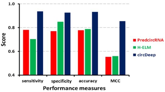
Comparison of circular RNA prediction tools: circDeep significantly outperforms previous proposed methods (see Section 3 for details)
2 Materials and methods
In this section, we describe our deep learning framework that integrates different sources of data to predict circRNAs. We describe a method for extracting distinctive representations of different sources, which are subsequently integrated using feature fusion learning to predict circRNAs.
2.1 Feature descriptors
2.1.1 RCM descriptor
Many studies support the idea that reverse complement matching in flanking introns and circularization are highly associated. Ivanov et al. (2015) demonstrated that reverse complementary sequences between introns bracketing circRNAs were notably elevated in comparison to linear controls. It has also been demonstrated that the presence of long inverted repeats (IR) flanking the mouse Sty genes results in the creation of the Sty circular transcript in cultured cells (Dubin et al., 1995). Zhang and colleagues provide several lines of evidence to support the deduction that circRNA formation is reliant on flanking complementary sequences, either with repetitive or non-repetitive components (Zhang et al., 2014). Consequently, it has been suggested that RCMs (Fig. 2a) encourage hairpin creation of the transcript which describes how an upstream acceptor site (3′ splice site) of an upstream intron is fastened to a downstream donor site (5′ splice site) of a flanking downstream intron. A feature like this can be a strong key feature to help our model predict the potential of a sequence to be transformed to circRNA.
Fig. 2.
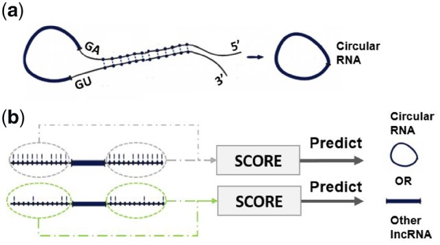
(a) Reverse Complement Matches between flanking sequences promote circularization of RNA. (b) Computing the strength of hairpin in flanking sequences allows circular RNA prediction
Therefore, we begin by deriving score H for computing the presence of reverse complementary sequences in flanking sequences. It represents the absolute number of all reverse complement sequences in the flanking sequences. Therefore, for each query sequence S, we take two flanking sequences, each of length base pairs (bps). We then split the two sequences into k-mers using the sliding window approach. We extract all subsequences of length with stride , resulting in L subsequences . There are possible words of length in the sequences. For each word in the vocabulary; , we count the number of occurrences in the left flanking sequence and the number of occurrences of the reverse complement to in the right flanking sequence . is the reverse complement of the word , for example = ACGGU.
Then the score of the sequence S is given by Eq. 1 which is the sum of scores of all words where is the absolute number of occurrences of the word :
| (1) |
where
Our score can be informative about the absolute number of reverse complement sequences. This can be very useful, according to current models for the production of circRNAs, which posit that RNA secondary structures formed by inverted sequences in flanking introns are necessary elements for circularization.
Dubin and colleagues have suggested that at least 400 complementary nucleotides are necessary for Sry circularization in vivo (Dubin et al., 1995). Other research (Hansen et al., 2013) has shown that artificially surrounding an exon with introns containing 800 nucleotides (nt) of perfectly complementary repeats is sufficient to allow circularization which suggests that long reverse complement sequences promotes circularization. Lacking detailed mechanistic models of circularization generally makes the prediction of circRNAs difficult but, based on some previous studies, we hypothesize that strengthening the hairpin between the reverse complement sequences may increase the likelihood of circularization. Therefore, the availability of a measure describing the longest reverse complementary sequence in flanking sequences to a query sequence for our classifier should improve discrimination between circRNAs and other lncRNAs.
In the following pseudocode, we describe our procedure for computing score V that describes the strengthening of the hairpin between flanking sequences. In the result section, we show the effectiveness of such a feature for discriminating circRNAs from other lncRNAs.
In order to evaluate the strengthening of the hairpin between flanking sequences (Fig. 2b), our method provides a new dynamic programming approach that computes score V for the longest reverse complement sequences while allowing some mismatches and penalizing non-complementary nucleotides. To calculate the longest reverse complement matching between two sequences of length and respectively, we split each sequence into overlapping k-mers of length with stride equal to 1, so each sequence is represented by , and respectively. RC(Wi) is the reverse complement of the word Wi, for example RC(ACGUG) = CACGU.
Let be the score for the longest reverse complementary matching between sequences and with allowing some mismatches.
Calculation of score
FOR
FOR
FOR
FOR
IF
ELSE
In our formulation of the score V, we are allowing some mismatches for longest reverse complementary matching between sequences. If it contains many mismatches, the score V will be low, which reflects flanking sequences less likely to form a hairpin and more likely to form circular RNA. The time complexity of our algorithm to compute is . We use k-mers for computing score V. As a constraint, at least 1 k-mer is matched between two flanking sequences. However, this algorithm can be extended to eliminate this constraint by simply taking k = 1. The choice of the hyper-parameters to calculate the score V such as match score, mismatch score, are based on preliminary experiments.
2.1.2 Conservation descriptor
The PhastCons (Mikolov et al., 2013) method is used to give a score ranging from 0 to 1 to each nucleotide based on its conservation level. We gather pre-computed conservation scores from the UCSC database (https://genome.ucsc.edu). For every exon sequence in every transcript, we average the scores in the exon sequence and then compute the maximum, the average and the median of those averaged scores. If a transcript does not have an exon, the entire transcript is held as a single exon for our computation.
CircRNAs have a multitude of conserved docking sites for miRNA such as ciRS-7 which holds over 70 selectively conserved miRNA target sites (Goldberg and Levy, 2014). This is a result of most circRNAs having almost identical motif sequences. Consequently, we sum the number of frequencies of successive bases whose scores are larger than the specified threshold and then divide the frequency by the whole length of the sequence. We alter the number of successive bases in the scope of 4 through 7, incrementing by 1 and setting a threshold in the range of 0.5 through 0.7, incrementing by 0.1. This gives us a total of 15 features to create our conservation descriptor.
2.1.3 ACNN-BLSTM sequence descriptor
In order to extract ACNN-BLSTM sequence descriptor, we build a deep learning architecture as shown in Figure 3 consisting of three main components: Embedding layer, Asymmetric convolutional neural network (ACNN) and Bidirectional long short-term memory (BLSTM) network.
Fig. 3.
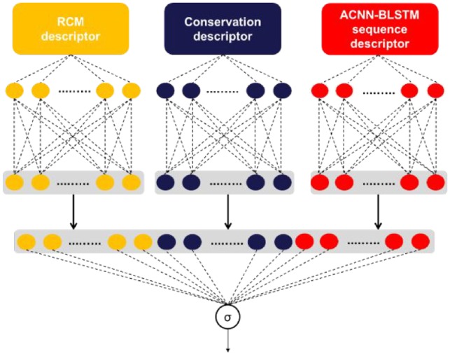
The flowchart of proposed circDeep for classification of circular RNA from other lncRNA. It extracts three descriptors and then use feature fusion learning to integrate different representations for classification
First, each sequence is converted to a sequence of k-mer indexes and then we map the k-mers to vectors found at the corresponding index in the embedding matrix. The embedding matrix is pre-trained first with the word2vec model (Mikolov et al., 2013) called skip-gram that computes the co-occurrence statistics of k-mer and learns to project them into a D-dimensional space Rd. It will be further fine-tuned during the training process.
As the convolution layer in our model requires fixed-length input, we pad each sequence that has a length less than maxlen with special symbols at the end that indicate the unknown k-mers and for those that have a length longer than maxlen, we simply cut extra k-mers at the end of these sentences to reach maxlen. So now, each sequence is represented as:
| (2) |
where be the d-dimensional word vector corresponding to the jth k-mer in the sequence.
A deeper network will generally have more representational power than a shallower network, but the training time and the greater number of parameters makes them difficult to train. The number of parameters can be greatly reduced with a minor loss in performance by the use of asymmetric convolutions (Szegedy et al., 2015), allowing for deeper models to be trained using the same resources.
We divide the more common rectangular convolutional filter into two separate steps. First we apply convolutions, followed by convolutions (Szegedy et al., 2015).
The convolution filter is applied to each k-mer in the sentence and generates corresponding feature
| (3) |
where is element-wise multiplication, is the bias and is a non-linear function. We chose the ReLU activation function, because it is known to perform well in CNNs We get the feature map
| (4) |
The convolution with filter in is applied to a window of features in the feature map to produce the new feature and the feature map
| (5) |
| (6) |
Dropout is then employed (Srivastava et al., 2014) to reduce overfitting. The output of the ACNN is read by a BLSTM, enabling long term dependencies to be captured in both directions.
Recurrent networks are especially well suited for finding dependencies and complex relationships in sequential data. However, they can only recognize very short-term dependencies. This problem is overcome using forget gates, which allow some information to be preserved for long stretches of time while selectively forgetting data that is not needed. In this task in particular, dependencies in both directions are important, so a BLSTM network is used to capture this.
2.2 Feature fusion learning for circular RNA prediction
Since we have different heterogeneous descriptors from different sources of data, feature fusion learning is incorporated in the model to learn shared features across different sources of data. The proposed model can learn and combine high-level heterogeneous representations simultaneously.
The first step in our method involves training the model described in Section 2.1.3 and computing the optimal parameters where is the number of hidden layers for ACNN-BLSTM architecture. Next, for each sequence, we compute the ACNN-BLSTM sequence descriptor using the feed-forward pass procedures by taking the final representation before the output layer. We extract, at the same time, conservation and RCM descriptors using methods described in 2.1.1 and 2.1.2.
The second step of our method involves teaching the model with the three obtained descriptors. To achieve this, we can utilize either ‘late fusion’ (decision fusion) or ‘early fusion’ (brute force feature concatenation). Early fusion takes features from the three modalities, chains them together, and then uses the new vector formed to train a deep neural network. The only issue with early fusion is that it fails to consider the different statistical properties of the information it concatenates together. Late fusion creates a final prediction, which is simply an amalgamation of each unimodal prediction from the three modalities. Each unimodal prediction has an output interpreted as a confidence score; these scores are combined to give us the final confidence score. The final prediction allows us to maximize the capabilities of each unimodal classifier; however this method loses some correlation in multi-dimensional space. To avoid this, we use a slight variation of late fusion called ‘feature fusion fine-tuned’ which is shown in Figure 4. In our variation, we put each information source through multiple layers to construct a high-level representation of each source. The final representation is just an amalgamation of each individual high-level representation.
Fig. 4.
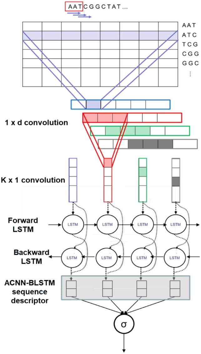
Graphical illustration of our end-to-end deep learning architecture used to extract ACNN-BLSTM sequence descriptor
While feature learning, individual DNN’s are trained beforehand separately and then fused together for the last common training which utilizes backpropagation. Learned parameters from each model are adjusted automatically during each training epoch. After multiple training epochs, the model can recognize depictions from the RCM, the ACNN-BLSTM sequence and the conservative descriptors for ensuing categorization. Additionally, the model is better able to learn features for each modality using backpropagation when various modalities are present. This method avoids various problems present in other methods of fusing such as struggling to recognize highly nonlinear relationships, superfluity and reliance between several descriptors, and over-fitting.
3 Results and discussion
3.1 Experiment setup
In order to gauge the capabilities of our deep learning model, we used human circRNAs from the database circRNADb (Hall, 2000) which contains 32 914 human circRNAs carefully selected from diversified sources. After we removed circRNAs shorter than 200 nucleotides, we were left with 31 939 circRNAs to act as our positive dataset. We used GENCODE (Zeng et al., 2016) to create our negative dataset which was made of other lncRNAs such as processed transcript, antisense, lncRNA, sense intronic and sense overlapping. The annotated lncRNAs in GENCODE have three validation levels for RNA annotation: validation, manual annotation and automated annotated. Only transcripts that were validated or manually annotated were chosen to obtain 19 683 samples that compose our negative data.
We then divided each dataset into training data, validation data and testing data where 75% were used for training, 10% for validation and 15% for testing. The training data was used to fit the optimal parameters for our model. We then used the validation data to test the performance of the model with these parameters. The test data was then used to test the model with the best performance on the validation data. The testing was used to provide an unbiased evaluation of a final model fit on the training dataset.
For the unsupervised training of k-mer embedding, we generated the corpus of k-mer sequences by setting k to 3, and the stride s to 1. Consequently, the k-mer vocabulary size was V = 43=64. Word2vec (Skip-gram with negative sampling) was implemented using efficient multicore implementation by Gensim (Tatomer and Wilusz, 2017), an open source Python library for processing large amounts of text with a focus on topic modeling. We set the window size (context) to 18, the length of the dense vector to represent each trinucleotide to 40, the initial learning rate to 0.025 and the number of iterations to 100.
circDeep is implemented in python using keras 1.0.4 which is found at https://github.com/fchollet/keras, with the backend of Theano (0.9.0) (Legnini et al., 2017). In order to benefit from the parallel computation of the tensors, we trained our model on a NVIDIA Tesla C2050.
To allow the deep architecture to extract an ACNN-BLSTM sequence descriptor, we set max length (maxlen) to 8000 bps, the number of asymmetric convolutional filters to 100, the filter length to 7, the memory dimension to 100, initial learning rate to 0.02, batch size to 128 and the maximum number of epochs to 45 (see Supplementary Table S1 for more details about architecture). This model is optimized using the RMSprop algorithm to learn all model parameters, including the convolution filters.
For the feature fusion learning, the number of hidden units for two fully connected layers (FCL) for each descriptor are listed in Supplementary Table S2. Batch normalization is added to all hidden layers. We set the initial learning rate set to 0.01, batch size to 64, the dropout rate to P = 0.3 and the maximum number of epochs to 70.
The evaluation measures used in the analysis included accuracy, sensitivity, specificity, F1 score and Matthews Correlation Coefficient (MCC).
3.2 Efficacy of RCM descriptor
To explore whether the new proposed features H(k, L0) and V(k, L1, L2) are able to predict circRNAs and improve the performance of our model, we used Pearson’s correlation score (Hall, 2000) to measure the relevance of these features and the dependence between the features and the class label (circRNA or other lncRNA). In other words, Pearson’s correlation score can be used to measure the capability that H(k, L0) and V(k, L0) features can discriminate between circRNAs and other lncRNAs. It is one of the most powerful feature selection techniques, and it is easy to compute and interpret. The resulting value lies in [-1; 1], with -1 meaning perfect negative correlation and +1 meaning perfect positive correlation. Higher scores equate to more relevant features.
We calculate H(k, L0) for k in the interval [3, 11] with stride of 1 and L0 in the interval [250, 2000] with a stride of 250. We calculate V(k, L1, L2) by taking the same length for flanking sequences L1 = L2 = L0 and varying it in the interval [250, 1750] with a stride of 250, and k is varied in the interval [1, 7] with a stride of 1. We set the matching score to 12 and the mismatch penalty to -2. The results for Pearson’s correlation for our proposed features H and V are shown in Figure 5. To make our results more rigorous, we also calculate the information gain for the same features (Supplementary Tables S3 and S4).
Fig. 5.
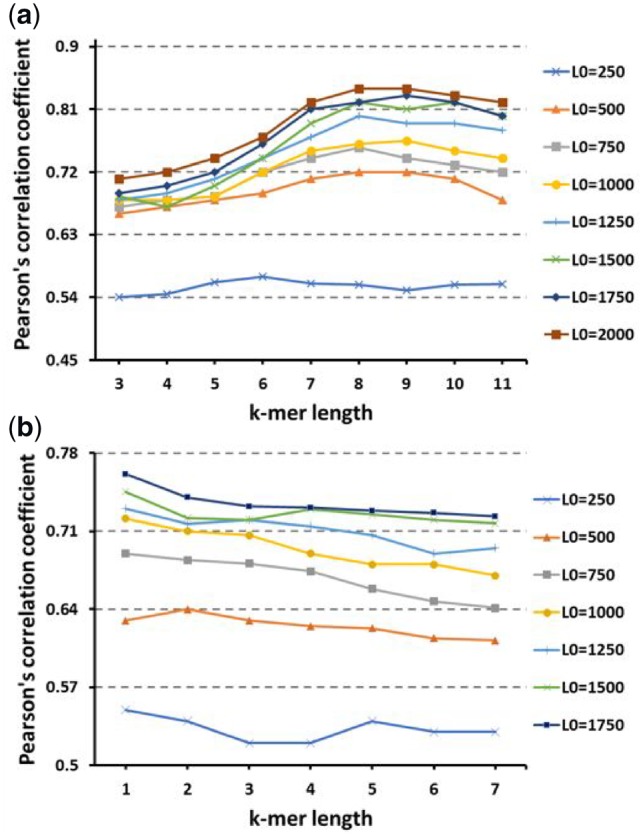
(a) Pearson's correlation coefficient as a function of H(k, L0) score for different k-mer length k and different flaking sequence length L0. (b) Pearson's correlation coefficient as a function of V(k, L0) score for different k-mer length k and different flaking sequence length L0
We can see that the results are very similar and give the same interpretation using any of the statistical methods. As can be seen in Figure 5, the Pearson’s correlations for H(k, L0) and V(k, L0) are considerably high, starting from 500 bps in the flanking sequences, indicating that the RCM that promotes the hairpin for circRNAs is mostly located after 250bps.
The results provide preliminary evidence to support our hypothesis that the features H(k, L0) and V(k, L0) for flanking sequences longer than 500bps facilitate the identification of circRNAs since most Pearson’s correlation scores are higher than 0.70 and can reach approximately 0.83.
It can be seen also from Figure 5 that Pearson’s correlation scores increase when the length of flanking sequences is increased for all values of k-mer length. However, these scores are not extracted for larger k-mer sizes and longer flanking sequences because the run time for both features, H(k, L0) and V(k, L0), is increased with the increased length and size (see Supplementary Tables S3 and S4).
When we compare features H and V for any fixed length of flanking sequences from Figure 5, H(k, L0) features reached better Pearson’s correlations scores than V(k, L0) features. This shows that the absolute number of RCM is more informative than the score of the longest hairpin in the flanking sequences when determining the likelihood of circRNA formation. Therefore, our results strongly indicate that circularization can be altered by the competition of RNA pairing across flanking introns and does not rely on the single longest reverse complement sequence.
Since we aim to obtain a robust classifier, we ranked the features using the Pearson’s correlation score and then selected the first 70 ranked features to obtain the final RCM descriptor composed of 42 H(k, L0) features and 28 V(k, L0) features.
3.3 Efficacy of ACNN-BLSTM sequence descriptor
3.3.1 Comparing with baseline architectures for sequence classification
To evaluate the efficacy of our proposed ACNN-BLSTM sequence descriptor, we compared the performance of our proposed architecture (Fig. 3) with several baseline methods for sequence classification. We compared with a one-hot CNN architecture adopted by (Zeng et al., 2016), a one-hot CNN-LSTM adopted in (Tatomer and Wilusz, 2017), a Glove-CNN-BLSTM adopted by (Min et al., 2017), a one-hot CNN-BLSTM, a one-layer LSTM, a one-layer Bi-LSTM, an ACNN and a CNN that we implemented (see Supplementary Table S5 for more details about each architecture).
Table 1 shows the accuracy on training and validation sets and the accuracy and MCC on the test set for all methods described above in addition to the number of epochs and average running time per epoch. By comparing different models, we noticed that convolutional neural networks (one hot-CNN, ACNN, CNN) outperform LSTM related models (LSTM, BLSTM); this validates the importance of convolutional operations in predicting circRNAs. The ACNN architecture is considered the fastest and the best among convolutional neural networks, it reached 0.833 accuracy and 0.6625 MCC on test data which demonstrates its power for capturing local sequence patterns and detecting spatial motifs that characterize the circRNAs. For LSTM related models, BLSTM architecture achieved best performance with 0.8020 accuracy and 0.5997 MCC. This indicates that it is more useful to have access to both, the past and the future context for predicting circRNAs.
Table 1.
Performance comparison between our ACNN-BLSTM proposed architecture and other baseline methods for sequence classification
| Method | Train | Val | Test | Test | #epochs | Time |
|---|---|---|---|---|---|---|
| ACC | ACC | ACC | MCC | |||
| One-hot-CNN | 0.8176 | 0.8185 | 0.8117 | 0.6164 | 24 | 368s |
| ACNN | 0.8402 | 0.8385 | 0.8330 | 0.6625 | 32 | 308s |
| CNN | 0.8225 | 0.8208 | 0.8194 | 0.6299 | 38 | 338s |
| LSTM | 0.7836 | 0.7820 | 0.7826 | 0.5568 | 24 | 712s |
| BLSTM | 0.8029 | 0.8034 | 0.8020 | 0.5997 | 31 | 748s |
| Glove-CNN-BLSTM | 0.8804 | 0.8756 | 0.8737 | 0.7324 | 48 | 354s |
| One-hot-CNN-BLSTM | 0.8609 | 0.8570 | 0.8541 | 0.6890 | 42 | 394s |
| ACNN-BLSTM | 0.8947 | 0.8935 | 0.8933 | 0.7730 | 36 | 347s |
The most interesting aspect of our results is how the performance is improved by combining a convolutional neural network with a recurrent neural network. This is not surprising when considering that recurrent neural networks excel at sequential modelling while convolutional networks completely fail at learning sequential correlations. Recurrent neural networks fail to derive features in parallel but convolutional networks can learn local responses from dimensional data. Consequently, the amalgamation of the two networks gives us both the benefits from the two and allows us to predict circRNA more accurately. Our method completely eclipsed the baseline models when predicting circRNA; it achieved 0.8933 accuracy and 0.7730 MCC on test data. We compared also the performance of all methods described above using 5-fold cross validation on training data, and the results are shown in Supplementary Table S6. We achieved almost identical results using cross validation and also when we ran validation and test data, which suggests that we have a low risk of over-fitting by using validation data and an early stop strategy.
3.3.2 Model analysis
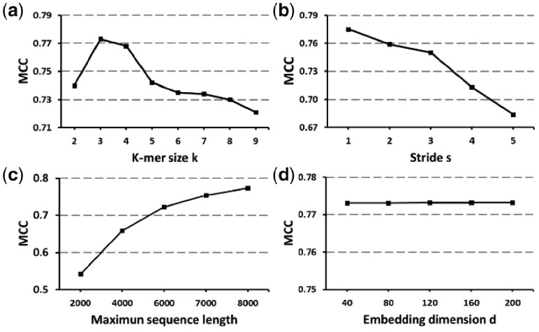
In order to analyze the aspect of our architecture used to extract the ACNN-BLSTM descriptor, we evaluated its robustness and interpreted the influence of four hyper-parameters: the k-mer length k, the splitting stride s, the maxlen parameter and the embedding dimension d. We evaluated our model using the MCC measure on the test set, and the results are shown in Figure 6.
Fig. 6.
Matthews Correlation Coefficient (MCC) scores for test data with varying four hyper-parameters
Starting with the k-mer length, k, we expected that increasing k would increase the total number of different k-mers, increase the information in the co-occurrence statistics and improve our model. However, we find that k = 3 gives the best performance. In fact, as the k-mer size increases, the performance decreases. This can best be seen in the significant drop in performance at k = 5. This leads us to the importance of mining the sequences with trinucleotides for circRNAs prediction. Even though circRNAs are classified as non-coding RNAs, recently, several studies demonstrate that circRNAs can be translated (Legnini et al., 2017; Pamudurti et al., 2017; Tatomer and Wilusz, 2017). In agreement with these findings, the peak at the k-mer size of 3, which is the size of one amino acid, in Figure 6a suggests that the translation of circRNAs is not trivial.
The second hyper-parameter is splitting stride, s. As expected, a larger stride will decrease the corpus size, which in turn, decreases the contained information in the sequence, and decreases the performance. Therefore, we set stride at s = 1 in our model.
The third hyper-parameter is maximum sequence length, maxlen. There is a positive correlation between MCC and maxlen. The reason behind the correlation is obvious, as some input sequences are truncated at shorter lengths, which results in a loss of information contained in the sequence. We were limited to a maxlen of 8000 bps, due to limitations in computer memory.
The final hyper-parameter is the embedding dimension d. We can see that it has no impact on the performance of the model, however, when d is increased, the time to train the weights of the embedding matrix is increased; this led us to choose d = 40 in our model.
Next, we investigated the impact of different filter configurations in the asymmetric convolutional layer on the model performance. In Figure 7, we show that the MCC measure on the testing data using different filter configurations. For each filter configuration, the best result under extensive grid-search on hyperparameters is shown in Figure 7. In the asymmetric convolutional layer of our model, filters are utilized to represent local trinucleotide features. We initially thought that several convolutional layers in parallel with filters of various sizes would perform better than any single asymmetric convolutional layer with filters of the same length due to different sized filters being able to find features of different n-grams (n consecutive 3-mers). However, our experiments demonstrated that a single convolutional layer with a filter length of seven always surpasses the other options. When multiple layers were run together, filter combinations with a filter of length seven always performed better. This further aided the verification of 7-g features playing a vital role in representing local features while predicting circRNA.
Fig. 7.
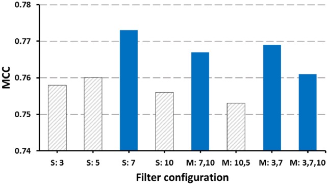
Matthews Correlation Coefficient scores for test data with different filter size strategies. For the horizontal axis, S means single convolutional layer with the same filter length and M means multiple convolutional layers in parallel with different filter lengths. In both single- and multiple-filter lengths, a filter of length 7 always showed higher MMC score (blue bars)
Seven-grams means we extract local features from every seven overlapping trinucleotides, which means three non-overlapping trinucleotides. This is in agreement with the results found in a study (Asgari and Mofrad, 2015) where using the word2vec skip-gram model was able to generate trigram of amino acids representations (one amino acid is equivalent to trinucleotide in DNA sequence) reproducing known physical relationships that were useful for protein classification. Our results show once again how circRNA sequences share characteristics with coding sequences when mining the sequences with text mining techniques where the sequence is treated as collection of k-mers.
3.4 Feature fusion performance for classification of circular RNA from other lncRNA
Table 2 shows the performance of unimodal classifiers, bimodal classifiers, multimodal classifiers and PredcircRNA. For unimodal classifiers, we stack two fully connected layers for each descriptor. For bimodal classifiers, we fuse two descriptors with each using our feature fusion approach. For multimodal classifiers, we fuse all three descriptors using feature fusion fine-tuned method described above, feature fusion by just the concatenation of the representations from individual trained DNN per descriptor without the tuning operation, early fusion and late fusion (see Supplementary Table S7 for performance comparison using 5-fold cross validation on training data). We also compared the time needed to extract all features on the test data, which contains 7630 samples. The comparisons were performed on an IBM desktop with 8 Intel Xeon CPU cores at 2.33 GHz and 24 GB memory.
Table 2.
Performance comparison between Unimodal classifiers, bi-modal classifiers, multimodal approaches and PredcircRNA
| Accuracy | MCC | F1 score | Time (min) | |
|---|---|---|---|---|
| SEQ | 0.8977 | 0.7792 | 0.8596 | 0.2 |
| CONS | 0.7611 | 0.4969 | 0.6897 | 15 |
| RCM | 0.7158 | 0.4072 | 0.64 | 27 |
| SEQ + RCM | 0.9263 | 0.8520 | 0.9268 | 47.2 |
| SEQ + CONS | 0.9333 | 0.8654 | 0.9333 | 15.2 |
| RCM + CONS | 0.8478 | 0.6838 | 0.8102 | 62 |
| Feature fusion fine-tuned | 0.9417 | 0.8833 | 0.9402 | 62.2 |
| Feature fusion | 0.9325 | 0.8653 | 0.9321 | 62.2 |
| Early fusion | 0.9271 | 0.8542 | 0.9278 | 62.2 |
| Late fusion | 0.9314 | 0.8628 | 0.9307 | 62.2 |
| PredcircRNA | 0.8056 | 0.6113 | 0.8108 | 515 |
SEQ, ACNN-BLSTM sequence descriptor; CONS, conservation descriptor; RCM, RCM descriptor; Time, time needed to extract features used for classification for test data. Bold ones are the best performer in each column.
As indicated in Table 2, ACNN-BLSTM sequence descriptor outperforms two other descriptors with an improvement of more than 15% in F1 score, which reflects its huge importance for our task. Even though our proposed RCM descriptor had the lowest performance capability with a high running time to be extracted, it was considered good with a 0.64 F1 score. We can also see its effect in improving performance when combined with other descriptors.
It is interesting that only 0.2 min is required to extract the ACNN-BLSTM descriptor with an 0.8596 F1 score, while PredcircRNA required approximately 8 h and 35 min to extract all features. This included graph features, component composition features, including frequencies of trinucleotides, conservation score features, features of ALU and tandem repeats, the ORF and SNPs from transcripts (GraphProt is taking most of running time) with only an 0.8108 F1. This reflects the importance of sequence patterns and long-range dependencies between trinucleotides in predicting circRNAs.
As expected, Table 2 shows that the multimodal fusion produces much higher performance than any individual modality. This indicates the strong complementarity shared between the three descriptors. Furthermore, feature fusion fine-tuned, which is adopted by circDeep, leads to a 0.9402 F1 score. This is greater than all unimodal learners and also other multimodal fusion baseline methods.
To once again make a comparison with PredcircRNA and H-ELM, we tested our tool with the data proposed by (Pan and Xiong, 2015), and the results are shown in Figure 1. This further supported our results and interpretations by having an improvement of more than 12% in accuracy using our proposed method.
4 Conclusions
In this paper, we propose a new multimodal deep learning tool circDeep to distinguish circRNA from other lncRNA. Compared to existing approaches, our approach has the following advantages: (i) It takes advantage of our proposed RCM descriptor which can provide the likelihood of circularization given the flanking sequences and the query sequences. (ii) It successfully integrates the ACNN, BLSTM and DNNs for dealing with the different input data types to enhance discrimination ability. (iii) The hybrid framework of flexible multimodal learning and fusion at an abstraction level makes our approach handle different features in an easy manner. The top-shared hidden layer at the fusion level will improve discovery of shared properties across different modalities. (iv) circDeep achieved an improvement of more than 12% in accuracy in both datasets with a very small running time compared to existing tools.
Supplementary Material
Acknowledgements
We would like to thank Eric Rouchka and Julia Chariker for insightful discussions and comments.
Funding
This work was supported by the KBRIN Investigator Development Award (IDeA) from the NIH National Institute of General Medical Sciences (P20GM103436) and NIH NIGMS AREA grant (R15GM126446).
Conflict of Interest: none declared.
References
- Asgari E., Mofrad M.R. (2015) Continuous distributed representation of biological sequences for deep proteomics and genomics. PLoS One, 10, e0141287.. [DOI] [PMC free article] [PubMed] [Google Scholar]
- Bachmayr-Heyda A. et al. (2015) Correlation of circular RNA abundance with proliferation–exemplified with colorectal and ovarian cancer, idiopathic lung fibrosis, and normal human tissues. Sci Rep., 5, 8057. [DOI] [PMC free article] [PubMed] [Google Scholar]
- Burd C.E. et al. (2010) Expression of linear and novel circular forms of an INK4/ARF-associated non-coding RNA correlates with atherosclerosis risk. PLoS Genet., 6, e1001233. [DOI] [PMC free article] [PubMed] [Google Scholar]
- Chen G. et al. (2012) LncRNADisease: a database for long-non-coding RNA-associated diseases. Nucleic Acids Res., 41 (Database issue), D983–D986. [DOI] [PMC free article] [PubMed] [Google Scholar]
- Chen L. et al. (2015) Circular RNAs in eukaryotic cells. Curr. Genomics, 16, 312–318. [DOI] [PMC free article] [PubMed] [Google Scholar]
- Chen L. et al. (2018) Discriminating cirRNAs from other lncRNAs using a hierarchical extreme learning machine (H-ELM) algorithm with feature selection. Mol. Genet. Genomics, 293, 137. [DOI] [PubMed] [Google Scholar]
- Cooper T.A. et al. (2009) RNA and disease. Cell, 136, 777–793. [DOI] [PMC free article] [PubMed] [Google Scholar]
- Derrien T. et al. (2012) The GENCODE v7 catalog of human long noncoding RNAs: analysis of their gene structure, evolution, and expression. Genome Res., 22, 1775–1789. [DOI] [PMC free article] [PubMed] [Google Scholar]
- Dubin R.A. et al. (1995) Inverted repeats are necessary for circularization of the mouse testis Sry transcript. Gene, 167, 245–248. [DOI] [PubMed] [Google Scholar]
- Eriksson M. et al. (2003) Recurrent de novo point mutations in lamin A cause Hutchinson-Gilford progeria syndrome. Nature, 423, 293–298. [DOI] [PMC free article] [PubMed] [Google Scholar]
- Goldberg Y., Levy O. (2014) word2vec Explained: deriving Mikolov et al.'s negative-sampling word-embedding method. arXiv preprint arXiv: 1402.3722.
- Hall M.A. (2000) Correlation-based feature selection of discrete and numeric class machine learning. In: Proceedings of the Seventeenth International Conference on Machine Learning, pp. 359–366.
- Hansen T.B. et al. (2013) Natural RNA circles function as efficient microRNA sponges. Nature, 495, 384–388. [DOI] [PubMed] [Google Scholar]
- Ivanov A. et al. (2015) Analysis of intron sequences reveals hallmarks of circular RNA biogenesis in animals. Cell Rep., 10, 170–177. [DOI] [PubMed] [Google Scholar]
- Lasda E., Parker R. (2014) Circular RNAs: diversity of form and function. RNA, 20, 1829–1842. [DOI] [PMC free article] [PubMed] [Google Scholar]
- Legnini I. et al. (2017) Circ-ZNF609 is a circular RNA that can be translated and functions in myogenesis. Mol. Cell, 66, 22–37 e29. [DOI] [PMC free article] [PubMed] [Google Scholar]
- Lukiw W.J. (2013) Circular RNA (circRNA) in Alzheimer's disease (AD). Front. Genet., 4, 307.. [DOI] [PMC free article] [PubMed] [Google Scholar]
- Mattick J.S., Makunin I.V. (2006) Non-coding RNA. Hum. Mol. Genet., 15, R17–R29. [DOI] [PubMed] [Google Scholar]
- Memczak S. et al. (2013) Circular RNAs are a large class of animal RNAs with regulatory potency. Nature, 495, 333–338. [DOI] [PubMed] [Google Scholar]
- Mercer T.R. et al. (2009) Long non-coding RNAs: insights into functions. Nat. Rev. Genet., 10, 155. [DOI] [PubMed] [Google Scholar]
- Mikolov T. et al. (2013) Efficient estimation of word representations in vector space. arXiv preprint arXiv: 1301.3781.
- Min X. et al. (2017) Chromatin accessibility prediction via convolutional long short-term memory networks with k-mer embedding. Bioinformatics, 33, i92–i101. [DOI] [PMC free article] [PubMed] [Google Scholar]
- Morel C.F. et al. (2006) A LMNA splicing mutation in two sisters with severe Dunnigan-type familial partial lipodystrophy type 2. J. Clin. Endocrinol. Metab., 91, 2689–2695. [DOI] [PubMed] [Google Scholar]
- Pamudurti N.R. et al. (2017) Translation of CircRNAs. Mol. Cell, 66, 9–21 e27. [DOI] [PMC free article] [PubMed] [Google Scholar]
- Pan X., Xiong K. (2015) PredcircRNA: computational classification of circular RNA from other long non-coding RNA using hybrid features. Mol. Biosyst., 11, 2219–2226. [DOI] [PubMed] [Google Scholar]
- Srivastava N. et al. (2014) Dropout: a simple way to prevent neural networks from overfitting. J. Mach. Learn. Res., 15, 1929–1958. [Google Scholar]
- Szegedy C. et al. (2015) Going deeper with convolutions. In: 2015 IEEE Conference on Computer Vision and Pattern Recognition (CVPR) pp. 1–9.
- Tatomer D.C., Wilusz J.E. (2017) An unchartered journey for ribosomes: circumnavigating circular RNAs to produce proteins. Mol. Cell, 66, 1–2. [DOI] [PubMed] [Google Scholar]
- Zeng H. et al. (2016) Convolutional neural network architectures for predicting DNA–protein binding. Bioinformatics, 32, i121–i127. [DOI] [PMC free article] [PubMed] [Google Scholar]
- Zhang X.-O. et al. (2014) Complementary sequence-mediated exon circularization. Cell, 159, 134–147. [DOI] [PubMed] [Google Scholar]
Associated Data
This section collects any data citations, data availability statements, or supplementary materials included in this article.


