Neuroimaging of Individual Differences: A Latent Variable Modeling Perspective

Abstract

Neuroimaging data is being increasingly utilized to address questions of individual difference. When examined with task-related fMRI (t-fMRI), individual differences are typically investigated via correlations between the BOLD activation signal at every voxel and a particular behavioral measure. This can be problematic because: 1) correlational designs require evaluation of t-fMRI psychometric properties, yet these are not well understood; and 2) bivariate correlations are severely limited in modeling the complexities of brain-behavior relationships. Analytic tools from psychometric theory such as latent variable modeling (e.g., structural equation modeling) can help simultaneously address both concerns. This review explores the advantages gained from integrating psychometric theory and methods with cognitive neuroscience for the assessment and interpretation of individual differences. The first section provides background on classic and modern psychometric theories and analytics. The second section details current approaches to t-fMRI individual difference analyses and their psychometric limitations. The last section uses data from the Human Connectome Project to provide illustrative examples of how t-fMRI individual differences research can benefit by utilizing latent variable models.

1. Introduction

For better or worse, there have historically been two very different research strategies taken in the study of human behavior (Borsboom et al., 2009; Cronbach, 1957): experimental and correlational (with the latter often referred to as the individual differences approach). Indeed, Cronbach (1957) expressed this distinction most cogently, “correlational psychology studies only variance among organisms; experimental psychology studies only variance among treatments” (pp. 681). Although these two strategies are not necessarily antagonistic, and in fact can be considered complementary or synergistic, in practice they have actually tended to remain quite isolated from each other.

Cognitive neuroscience borrows heavily from the experimental psychology tradition, which aims to understand the general laws of behavior by leveraging controlled experimental paradigms. The experimental approach involves systematically manipulating at least one independent variable (e.g., group or condition) to examine its effect on a given dependent variable of interest, typically by assessing differences in central tendency (e.g., mean). Likewise, in one of the primary methods used in cognitive neuroscience research – task functional magnetic resonance imaging (t-fMRI) – the most common analytic framework is a tightly controlled experiment in which two or more groups (or conditions) are compared across some measure of central tendency of the blood oxygen level-dependent (BOLD) activation signal (e.g., differences in between-group or condition means). Critically, analysis of central tendencies means that any subject-to-subject differences are treated as noise and collapsed into the central tendency, potentially obfuscating important information about variation across individuals. For instance, although a specific pattern of brain activity (or lack thereof) might be observed in the group as a whole, it may not reflect any given individual within that group (Miller et al., 2002). The Simpson’s paradox is a related, though not identical, demonstration of this issue, wherein the direction of association between variables at the population level is exactly opposite to the direction of association between these variables within the population’s sub-groups (Kievit et al., 2013; Simpson, 1951).

The other research tradition, and one less utilized in cognitive neuroscience, is individual differences psychology (as mentioned above, it is sometimes referred to as “correlational” or “differential” psychology). Here the goal is to identify the specific dimensions of behavior on which humans differ, and examine how these dimensions relate to other aspects of behavior. Individual differences studies are often (though not always) correlational in nature, trying to measure the association between variables. There is no evaluation of central tendency, as instead individual differences studies capitalize on the between-subject variability rather than differences between groups or conditions¹.

The primary focus on experimental manipulations within cognitive neuroscience, rather than on individual differences, has important implications for understanding the relevance of using group level results to inform the development of treatment approaches. Interventions developed to address dysfunctional neural systems or cognitive impairments need to be effective at the individual level. Thus, it is necessary to understand more directly how individuals vary in the way that their brains respond during various cognitive task states. While there have been many t-fMRI studies that use correlational methods to evaluate individual differences, the psychology sub-discipline of psychometrics has developed statistical modeling techniques that are aimed at explicitly addressing individual differences questions. Thus, this psychometric perspective has high relevance, but currently relatively low familiarity and impact, for cognitive neuroscientists interested in investigating individual differences questions. The purpose of this review is to discuss the ways in which neuroimaging research, especially work focused on task-related BOLD activation, can be enhanced by increased cross-fertilization with the methods and theories of psychometrics.

There are three main portions of this review. The first gives an overview of relevant topics from psychometric theory, and further discusses the statistical frameworks used by psychometricians for addressing individual differences questions. The second section offers a historical perspective regarding how individual differences in t-fMRI have been analyzed, and conversely, discusses the limitations of these current approaches from the psychometric perspective. The last section provides illustrative examples conducted on publicly available data (from the Human Connectome Project) to demonstrate how frameworks from psychometric theory can be directly applied to the analysis of t-fMRI brain-behavior relationships as tools for enhancing research in this domain.

At the outset, it is worth clarifying the topics that will not be included in this review in order to minimize excessive length. First, for the purposes of this review, the term “individual differences” will be defined as between-subject differences. One could alternatively consider this review to be on inter-individual differences, as opposed to intra-individual differences, with the latter focused on questions relating to how a single individual differs from him/herself in various contexts. Second, the focus of this review is to provide both a theoretical foundation and practical implementation of psychometric methods for t-fMRI BOLD activation studies; there will be little attention given to task-related or resting state connectivity, though some of this work may be cited as applicable and many of the issues discussed here apply to that literature as well. Third, this paper is devoted to analytic methods conducted after typical pre-processing procedures. See Dubois and Adolphs (2016) for further reading regarding technological advancements in MRI hardware and pre-processing specific to individual differences. Finally, t-fMRI is only one tool in a cognitive neuroscientist’s arsenal for investigating neural activation patterns; other methodological techniques include electroencephalography (EEG), magnetoencephalography (EEG), positron emission tomography (PET), transcranial magnetic stimulation (TMS), and so forth. This review is primarily concerned with t-fMRI, given its popularity in cognitive neuroscience research. However, it is noteworthy that principles originating from psychometric theory are relevant for all measurement tools in psychology and neuroscience, and should therefore be highly applicable to other non t-fMRI or multimodal methods. Accordingly, the core tenants presented here may be pertinent at a broader level, despite the scope of the review, and subsequent examples, remaining fairly narrow.

2. Individual Differences and Psychometric Theory

2.1. What is Psychometrics?

Scientific investigation into the cognitive functioning of living humans can be especially difficult to operationalize, since the constructs of interest are not directly measurable. When measuring the temperature in a vat of liquid, for instance, one can safely presume that there is some element of transparency between the thermometer reading and the actual temperature. Likewise, in single unit recordings of neurons, a microelectrode (placed intracellularly or extracellularly) records the voltage change over time as a neuron generates an action potential, and as such there is almost never a question as to what exactly the electrode is recording; it is a direct measurement of current generated by an action potential. Yet the relationship between a measurement tool in cognitive neuroscience and the behavior of interest is more opaque. For example, in the widely used N-back task of working memory (Braver et al., 1997; Gevins and Cutillo, 1993), participants must press a target button or key when the item presented on the current trial is the same as the item presented a certain number of trials beforehand (e.g., X-G-X for a 2-back condition). Working memory function is then measured in terms of accuracy and/or reaction time. Importantly however, accuracy and reaction time during the N-back are not a direct measurement of working memory. Rather, they are indirect measurements, or proxies, of a working memory construct. Similarly, BOLD imaging is an indirect measurement of neuronal firing. Neuronal firing elicits a hemodynamic response such that oxygenated blood levels quickly increase for populations of recently-active neurons. Doing so changes the relative ratio of oxygenated to deoxygenated blood, which can then be detected by the MRI scanner since oxygenated and deoxygenated blood have differing magnetic susceptibilities. In t-fMRI then, an increase in the BOLD signal in a particular region during a particular task is inferred to reflect activation in the neural populations located in that region in response to the task demands. Like the N-back and working memory example above however, the BOLD signal exploited in t-fMRI serves as a proxy, not a direct measurement, of neuronal activation. Indeed, it is now well-appreciated that there are many complexities in the relationship between neuronal firing and BOLD activation (Logothetis, 2008).

Since it is nearly impossible to directly measure a cognitive behavior, how would a researcher know if they are actually tapping the cognitive construct of interest? How can one be sure that that the N-back is assessing working memory rather than another related construct, such as general fluid intelligence or the fluency of perceptual processing? Ultimately, how does a researcher know if a measurement tool (e.g., survey, task paradigm etc.) is “good”? These types of questions form the backbone of psychometrics. As a field, psychometrics is concerned with how to quantify and measure behavior. It is the science of constructing and evaluating measurement tools in order to operationalize the study of psychological phenomena. Critically, psychometric considerations are paramount to the study of individual differences. In order to fully appreciate this, it is worth diving into the principles and applications of psychometric theory from a historical perspective (Classical Test Theory) and a modern perspective (latent variable modeling). The focus here will be on how reframing classic psychometric ideas with modern frameworks can yield more sophisticated approaches to studying cognitive individual difference. Later sections (i.e., Section 3) will then return to the relationship between psychometrics and individual differences as applied to t-fMRI.

2.2. Core Psychometric Tenets and Classical Test Theory

One can find Classical Test Theory (CTT), at least in part, in nearly every introductory psychology book, and a majority of the applied psychometrics research conducted in the cognitive sciences takes the CTT perspective. At the heart of CTT (sometimes referred to as “true score theory”) is the notion that one can never directly measure an individual’s “true” score on a given test because of the unavoidable problem of measurement error. The term “score” reflects the numerical value obtained by the measurement tool; common scores in cognitive neuroscience include accuracy, reaction time, a Likert scale value, a questionnaire response, or even the value of the BOLD signal. Researchers directly measure an observed score (X), which is a function of the individual’s true score (T) and random measurement error (E; X=T+E). In this light, a person’s true score is the expected value of the score if the test were administered over an infinite number of times.

In CTT, a measurement tool must demonstrate three hierarchically organized psychometric qualities in order to be considered “good”: variability (or discriminating power), reliability, and validity. Variability is the most basic, necessary psychometric quality and refers to how well a tool can produce different scores for different people (P. Kline, 2015). A measurement tool with zero variability is effectively useless in the study of individual differences (as well as group differences). For instance, consider a 10-item survey designed to assess happiness. If all participants answer identically, then the researcher learns nothing about how happiness varies across different individuals. Instead, the researcher is essentially multiplying each individual by the same constant. Therefore, a tool must first produce a sufficient range of scores, while also avoiding ceiling and floor effects (which introduce a more subtle restriction on variability; Lord and Novick, 1968).

The second psychometric quality in the hierarchy is reliability. Reliability asks if the variable scores produced by the measurement tool are consistent. In the context of CTT, reliability is the ratio of true score variance to the total observed variance. Should a test be particularly subject to measurement error (which is considered random in CTT), there would be little true score variance relative to the total observed variance and reliability would be low. There are four approaches to estimating reliability from the CTT perspective: internal consistency reliability, test-retest reliability, parallel forms reliability, and inter-rater reliability. The two most relevant types referenced in this review are internal consistency reliability and test-retest reliability. Internal consistency reflects the degree to which the item responses (or trial responses) within a test are consistent, and is typically measured by Cronbach’s alpha. The degree to which test scores are stable across time is known as test-retest reliability, and is typically measured via Pearson correlation (for two time points only) or intraclass correlation coefficient (ICC; Shrout and Fleiss, 1979; see Caceres et al., 2009 for how ICC is used in fMRI). Importantly, one cannot have a lot of true score variance if there is little variability to begin with.

The third psychometric quality at the top of the hierarchy is validity. There are numerous subtypes of validity: construct validity, discriminant (or divergent) validity, predictive validity, statistical conclusion validity, internal validity, and external validity, just to name a few. A nuanced discussion of the differences between the various types of validity is beyond the scope of the current review. Pertinent here are two points: 1) the broad definition of validity, and the one used throughout this article, is that validity asks if the test measures what it intends to measure, and 2) a measurement tool cannot be valid if it cannot produce reliable scores. Thus, validity is dependent upon reliability, which in turn is dependent upon variability. The CTT approach to measuring validity is via test-criterion correlations, which are correlations between test scores and scores on some criterion measure (e.g., a behavioral measure already assumed to reflect individual differences).

2.3. Transition from Classical to Modern Perspectives

While CTT can be very useful for conceptualizing the importance of these three psychometric qualities, especially reliability, CTT is also extremely limiting. CTT assumes that all measurement error is random and does not provide a clear avenue for addressing sources of systematic error. This is especially problematic in cases where known sources of error exist; for instance, a multicenter study would want to specify study site as a known source of potential variance. In response to this major pitfall of CTT, psychometricians have developed numerous frameworks that revolve around understanding latent variables.

2.4. Latent Variable Modeling

While the primary goal of CTT is to obtain a person’s true score on a test, the primary goal of latent variable modeling is to define and examine the relationship between an unmeasurable, latent construct and observable, measurable test scores (Borsboom et al., 2003). Consider some of the challenges in measuring working memory on a task such as the N-back. Here, working memory is the latent variable of interest, or the unobserved construct (usually represented by circles or ellipses; Figure 1), and accuracy and reaction time during N-back performance are considered manifest variables, or observed variables (usually represented by rectangles or squares; Figure 1). Latent variable analytic methods try to find a set of latent variables that satisfy the local independence principle, which states that a latent variable can fully explain why observed variables are related to each other. That is, the reason two measured variables can correlate with each other is because they are caused by the same latent variable and thus share some amount of variance. If that shared variance is partialled out (and attributed to the latent variable), then the two variables will be independent of one another. The manifest variables are thus dependent upon the latent variable. Directional regression lines from the latent variable to the manifest variable represent these relationships (Figure 1).

Figure 1.

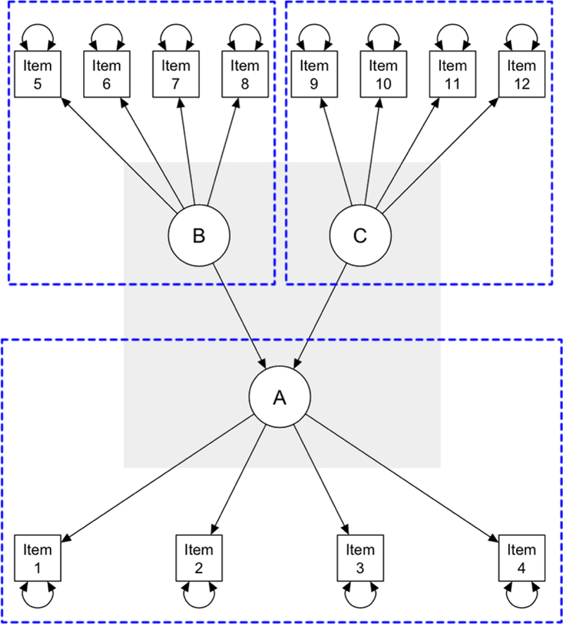
SEM schematic. Three measurement models (outlined with dashed blue boxes) are shown: manifest variables (squares) Items 1 – 4 loading on to latent variable (circle) A; Items 5 – 8 loading onto latent variable B; and Items 9 – 12 loading onto latent variable C. Curved, double-sided arrows reflect residual variances (not shown for latent variables for simplicity). The structural latent variable model model (gray background) reflects relationships between latent variables A, B, and C (straight regression lines).

There are a number of variations of latent variable analyses (e.g., structural equation modeling, latent class analysis, item response theory, latent profile analysis etc.); these differ primarily in terms of the type of data being analyzed, such as categorical versus continuous. The focus of this article is on structural equation modeling (SEM) as it is typically more appropriate in cognitive neuroscience contexts, seeing as many manifest and latent variables within the field are continuous (e.g., reaction time, the BOLD signal etc.). It is worth noting however that there is an effort to highlight a common framework for latent variable analytics (or a “unified approach”), rather than conceptualizing the methods as independent from each other (Bartholomew et al., 2011). Although further discussion here will remain on SEM concepts, these notations are still relevant to the broader application of latent variable modeling.

SEM (sometimes known as covariance structure modeling) is a rapidly growing analytic approach (Tomarken and Waller, 2005) that stems from factor analysis in the intelligence literature (Spearman, 1904) and path analysis in the genetics literature (Wright, 1921). Moreover, SEM itself encompasses a number of techniques including: confirmatory factor analysis, mediation analysis, path analysis, and latent growth modeling (see Figure 1 of Karimi and Meyer, 2014 for how different techniques under the SEM umbrella relate to each other, as well as for a more complete history of SEM). SEM asks whether the hypothesized relationships between latent variables and manifest variables, as well as latent variables and other latent variables, “match” or are consistent with observed data (Bollen, 1989; R.B. Kline, 2016). This is done by comparing the variance-covariance matrix of the hypothesized, implied model to the variance-covariance matrix of the observed data, often using a maximum likelihood function for estimating model parameters. Ultimately, one can conceptualize SEM as a series of simultaneous regression equations relating observed and latent variables to each other. SEM is typically employed in a theory-driven manner: the researcher describes the theory in an a priori manner by specifying how observed variables ought to organize into latent constructs (the measurement model, which alone is akin to a standard confirmatory factor analysis), and how these latent factors ought to correlate with each other (the structural latent variable model). Relationships between latent variables can be directional (regression equations) or non-directional (correlations or covariances; usually notated via curved lines with arrowheads on both sides). Finally, one can easily conduct group comparisons within the SEM framework since SEM is ultimately an extension of regression (and therefore ANOVA). Of note, while SEM is often utilized as a confirmatory approach, it is possible to use SEM in an exploratory manner. Since the more common application of SEM is confirmatory in nature, we will refer to SEM as a confirmatory procedure for the duration of this article (readers interested in exploratory SEM are directed to Lo et al., 2016 and Gates Molenaar, 2012 for further information).

There are many advantages to using SEM that make it a powerful tool when applied to individual differences questions in neuroimaging (see also Lahey et al., 2012). First, and perhaps most important, SEM allows researchers to directly test hypotheses about the sources of between-subject variability. Rather than accepting that there might be systematic unexplained variance in a measurement, SEM provides a framework to mathematically model these different sources of variance, thus giving researchers the flexibility of testing intricate models. For example, neuroimagers can specify different scanners or study sites as sources of variance, or even constrain specific model parameters if previous research supports doing so (e.g., a priori setting the relationship between any two variables to be zero if no association is expected, or set two parameters to be equivalent). Second, although SEM is flexible enough to be utilized in many different scientific contexts, it can be directly optimized for the study of individual differences by treating between-subject variability as the primary source of data for defining latent constructs. Third, because SEM is typically conducted in a confirmatory manner, it is well-suited for testing theoretical hypotheses. This is in contrast to exploratory methods like principal component analysis and partial least squares, which have been used in prior neuroimaging individual difference contexts (Krishnan et al., 2011), but are not designed for formal hypothesis testing. Fourth, latent variables defined in SEM are considered “error-free” in the measurement model component, in that they reflect the variance shared by multiple manifest (sometimes known as “indicator”) variables. If there is variance shared across some number of manifest variables, then by definition that variance cannot be random error (random error cannot correlate with anything). Fifth, SEM procedures often emphasize the goodness-of-fit of the overall model. A hypothesized model is deemed “good” if it adequately fits the data (e.g., does the model-implied variance-covariance matrix match the observed variance-covariance matrix?) and makes sense in a broader theoretical context. These fit indices can act as stand-alone criteria by which researchers can assess their findings, or they can be used to complement significance testing of particular path coefficients (which may or may not be of interest to the researcher). There are numerous model fit statistics, and though the specifics of each fit index are not relevant to the current discussion, one will commonly find the following indices in the literature: Chi-Squared, Comparative Fit Index, Tucker Lewis Index, Root Mean Square Error of Approximation, Standard Root Mean Square Residual, Akaike Information Criterion, and Bayesian Information Criteria. Further, SEM is a disconfirmatory procedure, in that a poor-fitting model can reject the hypothesized relationships between latent and manifest variables, but a well-fitting model does not mean that the hypothesized model is inherently correct, though the SEM framework does allow for comparison across competing nested models (see Section 4.2 for examples of nested model comparisons). For more information on SEM theory and application, see Bollen (1989) and R.B. Kline (2016).

Perhaps most vital for the current discussion is that SEM, and latent variable modeling more generally, offers psychometric improvements over other statistical techniques. SEM procedures are widely used to assess various types of validity. For instance, in the domain of working memory, SEM approaches can be (and have been) used to define latent variables derived from various popular task paradigms (e.g., N-back, Operation Span, etc.) and then relate these to other constructs and outcome variables, such as fluid intelligence, processing speed, inhibition, etc. (Conway et al., 2002; Engle et al., 1999; Kane et al., 2004). As another example, see MacDonald et al. (2005) for how similar SEM techniques have been used to assess convergent and divergent validity of a well-known experimental paradigm of cognitive control (the AX-CPT). Assessing reliability is less straightforward in SEM than from the CTT perspective, but the idea is that since the latent variable is error-free, a latent variable must then be capturing the “true”, replicable variance and is thus reliable. Reliability of individual manifest items is usually considered via “communalities” (or squared multiple correlations of factor loadings), reflecting the percent of variance in the manifest item that can be explained by the latent factor. These are useful in determining model specification errors in scenarios where the hypothesized models do not adequately reflect the observed data.

One of the biggest downsides of SEM is also its greatest upside. While researchers can test incredibly complex and nuanced models in a seemingly parsimonious manner, it comes at the expense of increased researcher degrees of freedom, as there are many additional parameters above and beyond traditional models. Thus, it is possible to get a well-fitting SEM model by just manipulating various parameters. To be fair, this type of overfitting also occurs in non-SEM analyses via selection of dependent variables and independent variables from a larger pool, employing covariates etc. (Simmons et al., 2011). However, SEM is more explicitly flexible, making it especially susceptible to overfitting concerns. Most SEM software provides a measurement of magnitude of change in the chi-square goodness-of-fit statistic should a new model parameter be specified. That is, the chi-square statistic could decrease by some number and therefore improve overall model fit if a new relationship is specified (often allowing indicator variances to covary). These are called modification indices. However, in the absence of a concrete, theory-based rationale for including the proposed modification, strict adherence to (or over-reliance on) modification indices can lead to problems with overfitting, generalizability, and interpretability (MacCallum et al., 1992). Fortunately, researchers can look to the goodness-of-fit indices mentioned above as benchmarks of when to stop adding new model parameters, as many fit indices penalize models for increased degrees of freedom. Some have even found that using overall fit indices along with modification indices can help identify important model parameters (Gates et al., 2011).

A second hindrance of individual differences methods, including but not limited to SEM, is that they require very large sample sizes in order to have sufficient statistical power, especially as the number of parameters to estimate increases. In SEM, n = 200 is often considered to be the minimum number of participants needed (Boomsma, 1985); however, see Wolf et al., 2013 for a more detailed discussion of appropriate sample sizes in SEM, and why a one-size-fits-all approach can be problematic for determining sample sizes. Despite these concerns, the advantages of SEM make it an ideal technique for undertaking individual differences questions.

The information presented thus far provides a solid basis of psychometric theory but does not fully make clear why psychometric considerations are so important for individual differences questions. Likewise, because of the relative lack of interaction between researchers versed in psychometrics and those working in cognitive neuroscience and task fMRI in particular, some of these considerations are not currently appreciated. To address this point, the aim of the next section is to delve more fully into explaining the relationship between psychometrics and individual differences as they relate to t-fMRI, as well as diving into why latent variable methods have not been widely adopted in t-fMRI. The final section of the article will then try to reconcile this discrepancy by providing several examples on how SEM can be applied to t-fMRI datasets.

3. Individual Differences in Task fMRI

The current standard analytic method for examining individual differences in t-fMRI activation studies is a simple correlation measure (Pearson or Spearman). Such an approach often starts with a whole-brain voxel-wise analysis that correlates BOLD activity in each voxel with an individual difference variable (either measured out of the scanner or in the scanner; Lebreton and Palminteri, 2016; Vul et al., 2009; Yarkoni and Braver, 2010). Voxels demonstrating significant correlations are clustered to define a region of interest (ROI) or set of ROIs, and the interpretation is that there is a significant brain-behavior relationship between the ROI(s) and the individual difference variable (note that there are a few studies that have tried to implement latent variable approaches – these will be discussed in section 4.1).

It is vital to appreciate that failure to understand a tool’s psychometric characteristics threatens the interpretation of individual differences conclusions. In a recent study, behavioral data from a cognitive control task (the AX-CPT) was used to directly demonstrate how interpretations might change in response to examining psychometric properties (Cooper et al., 2017). The following expands upon this notion by considering the three core psychometric requirements (i.e., variability, reliability, and validity) in the context of t-fMRI, and ends on a discussion of why psychometrics and cognitive neuroscience have not been fully integrated.

3.1. Individual Differences Questions Are Psychometric Questions

Variability:

A measurement tool without variability is ultimately useless in the study of individual differences because it provides no information regarding how individuals differ. While to the authors’ knowledge there has not been any overt concern that the BOLD signal does not generate enough variance per se, there has been much interest in the ways analytic approaches treat different sources of variance because aptly modeling sources of variability allows for statistical inference from the sample to population level (note that there have been a few attempts to visualize regional differences in variability; Omura et al., 2005). For example, switching from fixed effects to random effects models in the late 1990’s was explicitly done in order to model a different source of variability (in this case, modeling between-subject variance rather than treating it as noise; Holmes and Friston, 1998). More recently, some have argued that typical t-fMRI experiments fail to appropriately model variability at the stimulus level (Westfall et al., 2017). Re-thinking how variability is treated has a rich tradition in psychometric theory. Take Generalizability Theory (or “G-Theory”; Cronbach et al., 1963) for instance. G-Theory expanded upon CTT such that, instead of using a single composite random error term, the ANOVA framework was utilized to estimate error contributions from various sources. As Barch and Mathalon (2011) discuss in their review, G-Theory as applied to a t-fMRI individual differences study could potentially estimate variance components from person, task run, test session, or study site (for multisite projects). Detecting sources of excessive error variance can not only improve precision of reliability estimates, but the information can also be used when planning future studies in terms of making optimal study design decisions.

Reliability:

Reliability is crucial for individual differences studies because it essentially places an upper bound on the ability of the measurement tool to detect an effect, as the correlation between any two tests will decrease as a function of the square root of reliability (Nunnally, 1978). Reliability in t-fMRI has been frequently discussed in the literature in recent years, and it is fair to say, at the very least, that reliability estimates are quite variable (Bennett and Miller, 2010; Yarkoni and Braver, 2010). Emphasizing the importance and growing popularity of this topic, there was a special issue of Cognitive, Affective, and Behavioral Neuroscience in 2013 dedicated to reliability and replicability (Barch and Yarkoni, 2013). Reliability in the context of t-fMRI can be extremely difficult to parse for a number of reasons. To be clear, the reliability peculiarities mentioned below are neither an exhaustive list of all the factors influencing reliability in t-fMRI, nor are they even necessarily the most important factors per se. They do however pose unique challenges from a psychometric and measurement theory perspective.

First, reliability in t-fMRI can be difficult to conceptualize due to the enormous amount of data collected on an individual subject from a single run of an experiment. It is not uncommon for a typical t-fMRI protocol to yield roughly 100,000 voxels across the brain per subject. Moreover, the BOLD data obtained from each individual voxel is a timeseries measured over the course of the scan sequence; thus, there is no single value for the BOLD signal in a given voxel. The dimensionality of t-fMRI can therefore be overwhelming. As such, a number of dimensionality reduction steps go into the final dependent measures that are used in individual differences analyses (e.g., timeseries modeling, general linear model estimation of effects of interest, spatial smoothing, voxel clustering etc.).

Additionally, reliability in t-fMRI is influenced by a large number of study design factors such as: cognitive task used, experimental paradigm (block vs. event-related designs), contrast type (e.g., task > rest vs. target>nontarget), if statistical thresholding was used, and time interval for test-retest procedures (Bennett and Miller, 2013). Furthermore, metrics quantifying reliability vary by type (i.e., internal consistency reliability vs. test-retest reliability), and acceptable/high levels of test-retest reliability do not guarantee acceptable/high levels for internal consistency reliability or vice versa. One must then prioritize which aspect of reliability to focus on based on the research question. To be fair, these issues are not unique to t-fMRI or even cognitive neuroscience. Yet they are still important considerations that must be addressed when planning a t-fMRI study.

There is also the difficulty of integrating the extra “spatial dimension” associated with t-fMRI measurement across spatially organized elements (voxels) into reliability frameworks. Consider, for example, a cognitive task administered to individuals outside the scanner. Reliability could be examined via internal consistency – how consistent were the reaction times on the same trial types throughout the duration of the task – and via test-retest methods – how consistent are the reaction times across time points. If the same cognitive paradigm is then administered while participants are in the scanner, one can still examine the internal consistency and/or test-retest reliabilities of the BOLD signal, but it only makes sense to do so in a particular region or set of voxels. Holding all else constant, a t-fMRI paradigm can potentially yield reliable results for one region of the brain and unreliable results for a different region of the brain. Even in the resting state connectivity literature (i.e., without imposing a task context), patterns of reliability have been found to vary by brain region (Laumann et al., 2015). Further, spatial scale may be a critical factor, such that reliability at the voxel level may differ from the reliability at the ROI level, which may be different than reliability at the brain network level. A slightly different take on this revolves around how consistent is the answer to the question: “where in the brain is the BOLD activation located?” This is related to the notion that reliability can differ based on task. Here though, the focus is on whether the task can consistently elicit activation in the same regions. This idea of “spatial reliability” adds an extra dimension to an already highly dimensional problem.

Validity:

It is difficult to gain new insights into human behavior if using an invalid measurement tool. The dominant concerns regarding validity in t-fMRI are inter-twined with concerns about reliability. There are threats to validity in t-fMRI data that go beyond reliability, however, and relate to issues such as: 1) artifacts such as movement (Power et al., 2012; Siegel et al., 2013),, although these are tend to be more of a concern in resting state connectivity procedures rather than task activation studies; and 2) generalizability. External validity in the psychometric literature specifically concerns topics related to generalizability (Mook, 1983). In t-fMRI, participants are required to lie still for extended periods of time in the scanner, which can be quite difficult. Data from participants with excessive movement are often discarded (including some frames, some runs, or even all data from the participant) despite these participants perhaps not being true outliers of the population under study. Likewise, for some participants, the particular context of lying prone and still in a highly noisy and unfamiliar scanning environment may significantly impact task performance (Van Maanen, 2016). Interestingly, there is a new movement calling for adopting predictive frameworks seen in machine learning in order to improve generalizability, since a variable showing significant explanatory power does not necessarily mean the same variable will show predictive power for generalizing to new observations (Dubois and Adolphs, 2016; Lo et al., 2015; Yarkoni and Westfall, 2017).

Related to the concept of validity is interpretability. The high dimensionality of t-fMRI data can make interpretability somewhat challenging. Typically, t-fMRI researchers use one of two methods for finding areas of the brain relevant to the behavior of interest: a ROI or a whole-brain voxel-wise approach. The ROI solution is to select areas of the brain in an a priori manner. While this helps immensely for interpreting findings, it also has drawbacks: 1) it depends on researchers already having a theoretical foundation that constrains which brain areas (or ROIs) to investigate; and 2) it could potentially lead researchers to miss meaningful findings, since the analysis intentionally does not include the whole brain. Whole brain approaches often use some combination of statistical testing of task activation with an element of dimensionality reduction (e.g., principal component analysis or clustering algorithms) to find the set of voxels with BOLD task-related activation associated with behavioral individual differences. The result of this approach is that a potentially large number of brain regions (or clusters of voxels) co-activate to give rise to a particular behavior.

As an illustration of this point, consider the use of principal component analysis (PCA) as a data-driven approach to dimensionality reduction across the set of brain voxels. For example, in a study with a parametric manipulation of some variable (e.g., working memory load), the PCA might be used to cluster voxels with similar load-related activation patterns. In this case, if the first principal component was extracted, the top 1000 voxels with the highest factor loadings might be kept and treated as those representing a particular activation pattern. For the purpose of this hypothetical, say these voxels were located randomly throughout the brain. How then would one interpret the between-subject variance in this latent component? The variance captured by the latent variable in this case is not theoretically informed and is thus not clearly interpretable beyond a simple “variance shared across random items (brain regions)”.

The interpretability problem here is that the co-activating voxels may not make sense in a broader theoretical context. In this example, and as further discussed below (see Section 4.2.1, Example 3), the question of validity must be addressed by thinking of whether the regions that are grouped together make sense with regard to some theoretical framework (i.e., does the grouping reflect known brain networks or pathways). Newer work from resting state connectivity may help ultimately alleviate this specific issue and enhance interpretability. Recent studies have shown that brain regions organize into networks (e.g., frontoparietal, default mode), and that these networks show similar organization across both “resting” states and “task” states (Cole et al., 2014; Gratton et al., 2016a; Power et al., 2014). Although functional networks have been defined using resting state fMRI, the assumption is that these networks are critical sub-units of the cortex, and thus these networks should also be identifiable and useful in task activation studies. Focusing on networks as the level of analysis seems like a particularly promising middle ground for t-fMRI studies, as the preserved data in networks maybe more robust, due to occupying a higher level of brain organization, than typical whole brain voxel-wise analyses, yet are broader and more flexible than ROI analyses.

All told, one cannot fully interpret individual differences findings without taking into account psychometric considerations. Cognitive neuroscientists striving to understand brain-behavior relationships must then grapple with psychometric concerns. Although the standard correlational procedure is not incorrect, its relative simplicity makes it difficult to test brain-behavior questions that might be more complex or nuanced. This raises the question of why have researchers using t-fMRI not utilized the analytic techniques put forward by psychometric theory? Though not the sole reason, the primary hindrance in employing latent variable models is that t-fMRI studies, historically, have had too few participants to afford the type of power needed for latent variable models. To this end, a recent study by Poldrack et al. (2017) examined how sample sizes in t-fMRI studies have changed between 1995 and 2015, looking at over 1,100 published studies. They found that between 1995 and 2010, the median sample size steadily rose from just shy of 10 subjects to just shy of 20 subjects, and further report that by 2015 the median sample size was 28.5 for single group analyses and 19 per group for multiple group analyses. Although this increase is heartening from the perspective of statistical power, these sample size numbers are shockingly low from the standard perspective of SEM studies, e.g., the Boomsma et al. (1985) recommendation of 200 participants. As such, perhaps it is not surprising then that many of the modern psychometric frameworks have not been adopted in the t-fMRI arena.

The importance of power cannot be overstated, and low power across all of psychological and neuroscience research has come under scrutiny in recent years (Button et al., 2013; Open Science Collaboration, 2015; Szucs and Ioannidis, 2016). But the problem is especially pernicious for individual differences t-fMRI research, even when using the correlational approach (e.g., Pearson or Spearman statistical test), since most studies use a threshold of around p < .001 (if not lower) for the whole brain portion of the analysis. As Yarkoni and Braver (2010) describe in relation to individual differences in working memory: “When one considers that a correlational test has only 12% power to detect even a ‘large’ correlation of 0.5 at p < .001 in a sample size of n = 20, it becomes clear that the typical fMRI study of individual differences in [working memory] has little hope of detecting many, if not most, meaningful effects” (p. 96). The small sample sizes and underpowered research thus undermine the reproducibility of t-fMRI studies (Turner et al., 2017). Since statistical power is important for all research, and especially vital for individual differences research, the following provides a brief history of sample sizes in t-fMRI in hopes of clarifying why t-fMRI studies to date have been so woefully underpowered.

3.2. A Brief History of Low Sample Sizes in t-fMRI

Before diving into the cultural and analytical underpinnings of small sample sizes in t-fMRI, it is worth pointing out that t-fMRI studies can be very costly and time-intensive, which could potentially explain why sample sizes were so small. However, cost alone does not justify the consistently low sample sizes in t-fMRI studies over the years. For example, a one-hour research MRI scan at Washington University in St. Louis prior to 2002 cost $200 an hour (equivalent to $278.73 after adjusting for inflation) and has steadily risen to $630 per hour in 2017 (S.E. Petersen, personal communication, September 12, 2017). The costs are therefore much higher now (at least at this institution), despite larger samples also being collected now (Poldrack et al., 2017). Furthermore, event related potentials (ERP) studies are more cost-efficient than fMRI, yet have similar patterns of small sample sizes (roughly 10–20; S. Luck, personal communication, June 20, 2018) and a similar lack of transparency in sample size calculations (Larson and Carbine, 2017). The historical use of small sample sizes in neuroimaging is thus clearly not entirely driven by cost; there must have been other factors.

In 1990, Ogawa and colleagues reported their discovery that the BOLD signal could be used as an endogenous contrast for identifying localized regions of neural activity, providing the foundation for the entire field of t-fMRI. Interestingly, they directly compared BOLD imaging to PET (positron emission tomography) imaging. Although PET is non-invasive, participants are exposed to ionizing radiation, and thus PET studies standardly have intentionally small sample sizes. For historical context, the first activation maps from PET were produced in the mid to late 1980’s — before t-fMRI (Fox et al., 1986; Lauter et al., 1985). Many researchers who began to utilize t-fMRI in the early to mid 1990’s came from the PET research traditions that included data collection on small sample sizes. To be clear, this is not true of every investigator, or even every institution. However, the cultural norms from PET studies certainly seem to have crossed over into the early t-fMRI studies. For example, the well-known fMRI processing software SPM was originally developed in order to analyze PET data — not fMRI data (Friston, 2007).

From the mid to late 1990’s, t-fMRI was primarily a between-groups endeavor. Between-subject variance was treated as error in fixed effects models, and the need for random effects models was not fully appreciated until the late 1990’s (Holmes and Friston, 1998; Braver et al., 1997). Yet random effects models are less powerful than fixed effects models, leading to the realization that studies adopting random effects models would be severely underpowered if using equivalent sample sizes as their fixed effects counterparts. Similarly, the need to correct for false positives was not immediately apparent, and the adoption of false positive corrections highlighted the fact that early t-fMRI studies were severely underpowered (Bennett et al., 2010).

By the early 2000s, the field saw an increase in questions surrounding individual differences (for example, see Figure 1 of Braver et al., 2010), though they remained secondary to experimental manipulations. In 2009, a landmark paper on “voodoo correlations” revealed that correlations being reported were exceedingly high; higher than mathematically possible given the reliability of the measurement tools (Vul et al., 2009). The authors attribute these exceedingly high correlations to the “non-independence” problem, or a form of statistical double dipping. Essentially, t-fMRI studies would set a threshold where significant voxels were grouped into a ROI, and then the same BOLD data used to create the ROIs were used in a subsequent selective correlational analysis (see also Kriegeskorte et al., 2009 for more on the non-independence problem in neuroscience). Although voodoo correlations may superficially seem unrelated to issues surrounding power, Yarkoni (2009) argued in a response to Vul et al. (2009) that the inflated correlations Vul et al. observed are not only caused by the non-independence problem, but that they are also due to the pervasively low statistical power in t-fMRI studies. Specifically, a direct consequence of low power is that finding a significant effect invariably leads to inflated effect sizes. Thus, while the non-independence principle may certainly have threatened earlier t-fMRI correlations, it is the repercussions stemming from low statistical power that likely drove the exceedingly large correlations, skewing individual differences studies and their inferences (Yarkoni, 2009).

By around 2010, the implications of low power were becoming more widely acknowledged (Yarkoni and Braver, 2010). Even still, however, there was interesting debate over appropriate sample sizes for t-fMRI (see Friston, 2012 for an argument in favor of smaller sample sizes, and Lindquist et al., 2013 and Yarkoni, 2012 for formal and informal rebuttals, respectively). Ultimately, the field seems to have accepted the need for larger samples, and is striving towards that end.

At present, it seems as though a cultural shift is finally arriving in the field, with researchers and funding agencies alike becoming determined to conduct adequately powered t-fMRI studies. In response to all of the power criticisms over the years, t-fMRI is heading towards a new “big data” era wherein pooled funding sources and data sharing infrastructure allows consortiums to collect data on very large samples that can be shared with investigators at various institutions. In the United States, the first project of this kind was the Human Connectome Project (HCP; https://www.humanconnectome.org), which collected advanced neuroimaging (structural and functional), cognitive and behavioral measures, and genetic markers on over 1,000 participants (Barch et al., 2013; Van Essen et al., 2013). Similar efforts have been ongoing in Europe, including the Cam-Can study (Shafto et al., 2014), and UK Biobank (Sudlow et al., 2015), and newer, more ambitious projects such as the Adolescent Brain Cognitive Development study (https://abcdstudy.org) are currently underway. For more on neuroimaging big datasets and their associated technical and practical hurdles facing big data, see Poldrack and Gorgolewski (2014) and Smith and Nichols (2018). After nearly 30 years, t-fMRI research is now in a position where analytic methods, such as latent variable modeling, that were once untenable due to low sample sizes, are now within reach.

Consequently, there is much to gain from engaging in collaborative efforts between psychometrics and cognitive neuroscience. Those trained in measurement theory are especially well-equipped to address questions surrounding difficult-to-measure phenomena. Conversely, cognitive neuroscience may be a new frontier for many psychometricians, offering new opportunities for applying psychometric theory, which will likely further drive development and refinement of new and more powerful frameworks. Yet cognitive neuroscience has so far remained relatively disconnected from psychometric theory. In fairness, it is not just cognitive neuroscience, as cognitive psychology is also not as well integrated with psychometrics as other sub-fields of psychology, such as educational psychology and personality psychology. Indeed, one could even argue that psychology itself is not well-integrated with psychometrics (see Borsboom, 2006 for an interesting take on this topic). Collaboration is also impeded by the fact that the field of psychometrics is smaller than the other psychology disciplines, and so has a narrower penetration than cognitive neuroscience. Yet despite the current separation of these fields, collaboration will be necessary in going forward to advance understanding of brain-behavior relationships.

4. Integration and Examples

Thus far, this review has taken a historical slant regarding the factors that have impeded the development of optimized individual differences approaches in t-fMRI. The remainder of this article will shift the spotlight towards how to remedy the situation going forward. The following first briefly explores the ways latent variable models have been previously used in t-fMRI. Next, seven concrete and simple examples are presented in order to illustrate some ways in which SEM can be harnessed for the purposes of discerning brain-behavior relationships. Of course, the exact ways in which SEM can be employed are entirely dependent on the question at hand. As such, we strived to reduce the complexity of the examples, in hopes that readers could see some similarities to questions they find interesting and ideally gain confidence in expanding upon these procedures in their own work.

4.1. Latent Variable Models and t-fMRI — What Has Been Done?

There are some previous studies that have used latent variable models like SEM in t-fMRI. Yet a common theme between studies that have used latent variable approaches is that many of them were not deployed from an individual differences perspective. In one of the earlier human studies, for example, the main goal of SEM was to see if effective connectivity changed as a function of working memory load (McIntosh et al., 1996). In the context in which the paper was published, individual differences were not of concern; in fact, additional corrections were applied to statistically control for individual variability, rather than exploit it (McIntosh et al. 1996). This was not uncommon. Additionally, a majority of the work using SEM in neuroimaging has been applied to connectivity, rather than activation, in trying to answer between-groups and interactions questions (Schlösser et al., 2006). While very interesting, it is also a different context from an individual differences study.

In a more recent study by Beaty et al. (2016), SEM was used to assess how individual differences in personality traits predict functional connectivity in the default mode network. Yet the focus here was on individual differences in personality traits, rather than using latent models to define individual differences in default mode connectivity (i.e., multiple indicators were used to create the latent personality traits, which were then regressed onto a single manifest default mode connectivity variable).

Lahey et al. (2012) provided a nice demonstration of how confirmatory factor analysis (a technique falling under the SEM umbrella) and SEM could explain how a hypothesized brain network (mesocorticostriatal system) might predict behavior (impulsivity). Here, the latent variable representing the mesocorticostriatal system reflected contemporaneous BOLD activation of multiple indicator regions (e.g., dorsal anterior cingulate, right ventrolateral prefrontal cortex, etc.). Importantly, they performed an element of dimension reduction by defining ROIs used in their CFA/SEM based on those regions that showed a main effect of task condition (card-guessing reward task). Their strategy was to first obtain contrast images for each individual subject (positive feedback > negative feedback); these contrast images were “then used in second-level random effects models accounting for scan-to-scan and participant-to-participant variability to determine group mean condition-specific regional responses” (p. 8). This approach to ROI definition is somewhat of a limitation, in that it may actually reduce the potential for finding individual differences effects. In particular, when ROIs are selected based on showing significant condition-related effects, this indicates a relatively consistent effect across subjects, since in condition-based contrasts, between-subject variability serves as the error term, and so will reduce statistical significance if it is too high. Conversely, statistical power will be maximal for detecting individual difference effects under conditions of high between-subjects variability. Thus, even though Lahey et al. (2012) determined that the mesocorticostriatal latent variable captured significant between-subjects variability, they may have had greater statistical power, or even a different pattern of results, if ROIs were defined in a manner that was unbiased to within vs. between-subjects variability.

Lastly, Kim et al. (2007) put forth the “unified” SEM framework, which posited that the first stage should be comprised of an individual SEM for every single subject using BOLD timeseries data, then researchers should merge the path coefficients from the individual SEMs with subject-level covariates (e.g., gender, education etc.), and finally use a general linear model to ask if the covariates impacted the path coefficients. This has been further expanded upon in the newer “extended unified SEM” or “euSEM” (Gates et al., 2011) to allow for modeling of experimental effects on ROI activation, as is needed in event-related designs. Though not inherently specific to individual difference analyses, euSEM has sometimes been applied from an individual difference perspective (Hillary et al., 2011; Nichols et al., 2013).

4.2. SEM in Practice – Examples

Seven examples are reported below in order to provide concrete demonstrations of how SEM can be applied to individual differences questions in t-fMRI. Examples are grouped into two primary groups to assist with readability: Measurement Models and Validity includes examples 1–3 and Brain-Behavior Relationships includes examples 4–7. All data come from the publicly available Human Connectome Project (1200 subjects release; details of task descriptions and preprocessing pipelines can be found at Barch et al., 2013 and Glasser et al., 2013, respectively). Working memory as a construct, and the N-back task as a measurement tool have been used as examples throughout this review thus far; accordingly, the imaging data used in following SEM example were collected during the N-back task, specifically the 2-back > 0-back contrast. To reduce dimensionality, we applied the parcellation algorithm described by Gordon et al. (2016) resulting in 333 cortical parcels that comprise 13 networks where each parcel contains the per person average “cope” (contrast of parameter estimate). Importantly, utilizing this parcellation algorithm avoids some of the non-independence issues mentioned earlier, since it implements a whole-brain perspective (though subcortical regions are excluded, these could easily be added as well) that defines regions according to a priori properties, and thus is totally agnostic to experimental manipulations that could complicate interpretations. That is, parcel boundaries applied by the algorithm were derived from resting state connectivity on a different dataset (Gordon et al., 2016), therefore eliminating the risk of statistical double dipping. The following examples will mostly deal with the frontoparietal network (FPN), which is comprised of 24 unique parcels. For ease and simplicity, we only include participants with complete data and therefore n=1017 for all analyses below. All procedures used a maximum likelihood estimator (see Supplement 1 for more details). Finally, all procedures presented here were conducted in R, primarily using two packages: 1) lavaan (Rosseel, 2012) was used for all statistical analyses and 2) semPlot (Epskamp, 2017) was used to create path diagrams for figures. Code for all of the following examples can be found in Supplement 1. Note that in cases where “big data” is not tenable, one might consider using a Model Implied Instrumental Variable (MIIV) estimation procedure, as it is robust to distributional assumptions and performs well with smaller sample sizes (Bollen, 1995; Bollen, 1996; Bollen, 2018). Those interested in MIIV may want to explore the MIIVsem R package, which integrates with the lavaan package (Fisher et al., 2017).

4.2.1. Measurement and Validity: Examples 1–3

4.2.1.1. Example 1 – SEM versus Averaging

4.2.1.1a. Brief Introduction and Analytic Approach

When faced with multiple variables that putatively index the same construct, a common practice is to simply average across the variables to create a single composite variable (i.e., in this case, an un-weighted average across all parcels). The SEM framework offers an alternative to the averaging approach. One downside to averaging is that any random variance that exists within the indicators is still captured, perhaps even compounded, in the composite score. Whereas with SEM, error (unexplained) variance is modeled separately from shared variance, thus effectively removing unexplained variance from the latent variable. As such, latent variables are often described as being “error-free” or having perfect reliability

To demonstrate this, we created two competing CFA models. For both models, indicators were all 24 FPN parcels, with one latent factor defined to reflect the FPN. Model 1a allows all loadings to be freely estimated. In this model, the latent factor FPN represents the between-subject variance that is shared across the 24 parcels. In Model 1b, all factor loadings are constrained to be one (path diagram not shown). Here, the latent factor FPN is formally almost equivalent to averaging the 24 parcels. Moreover, the benefit of using an alternative model (1b) in which all factor loadings are constrained to be equal to 1, rather than obtaining a true average, is that a chi-square difference procedure can be employed to directly compare nested models (i.e., a model in which one or more free parameters are fixed is considered a more “restricted” model and is thus nested within the full/unrestricted model – Model 1b is nested within Model 1a). We report four estimates of overall fit: Comparative Fit Index (CFI), Tucker Lewis Index (TLI), Root Mean Square Error of Approximation (RMSEA), and Standardized Root Mean Square Residual (SRMR). Finally, a chi-square difference test was conducted to statistically compare Model 1a to Model 1b.

4.2.1.1b. Results

The constrained model (i.e., the model equivalent to a CTT average; Model 1b) fit significantly worse than the freely estimated model (Model 1a; Δχ²(23) = 732.08, p < .001). Importantly, there is a great deal of heterogeneity in the factor loadings for Model 1a (ranging from .32 - .79; Figure 2a), indicating that all parcels within the FPN do not contribute equally to the shared latent variance component. Overall fit was poor for Model 1b (CFI - .71, TLI - .71, RMSEA - .12, SRMR - .17). Model 1a showed a clearly superior fit, yet by the primary criteria would still not be judged a satisfactory model (CFI - .78, TLI - .76, RMSEA - .11, SRMR - .07). Ideally, the CFI and TLI should be .9 or above (higher is better) and the RMSEA and SRMR should ideally be below .08 (lower is better).

Figure 2.

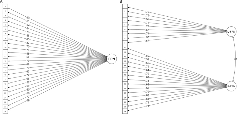
SEM path diagrams for Example 2. Model 2a (right) treats the FPN as a single, unified network (this path diagram also corresponds to Models 1a and 3a). Model 2b (right) splits the FPN network into lateralized sub-units (right FPN and left FPN). The correlation between right FPN and left FPN latent variables is shown via curved double-sided arrow. Standardized factor loadings are shown for both.

4.2.1.1c. Implications

The fact that fit indices reported above did not meet acceptable fit index thresholds may be indicative that Model 1a is too simple to fully capture the full structure of the data. The model fit can be improved by examining the modification indices (as described in section 2.3). Another option is to take an a-theoretical approach and let all residual variances of all indicators covary. However, as discussed in section 2.3, employing modification indices can be problematic in that doing so does not really address the underlying issue of the model not representing the data accurately. Additionally, researchers may choose to slightly modify the measurement model with procedures such as removing indicator variables with very low loadings (often <.50) or constraining some model parameters. Since the goal for the current review is to demonstrate how SEM can be used in the context of neuroimaging and the review is not intent on testing specific hypotheses constituting original research, we explicitly do not include correlated residuals of indicators or remove indicators with low factor loadings, at the cost of worse model fit, in an effort to keep these examples as simplistic as possible. As such, interpretation of fit indices should be relative to the models being compared (i.e., Model 1a’s fit indices were statistically better than Model 1b’s).

Overall, these findings indicate that the full model (Model 1a) where factor loadings were freely estimated was better than the restricted model (Model 1b), which essentially treated the latent FPN variable as an average of all 24 parcels. This suggests that an unweighted average approach is not the optimal way of combining parcel variables for assessing the FPN. If instead one utilizes the freely estimated SEM approach, the latent FPN variable should contain less error variance, which in turn should yield greater predictive power. We will return to this idea in Example 4, where we will incorporate measurement models and the relationships amongst latent variables. Examples 1–3, however, focus exclusively on measurement models (i.e., CFA).

4.2.1.2. Example 2 – Lateralization of the FPN

4.2.1.2a. Brief Introduction and Analytic Approach

Some previous work suggests that instead of being a unified network, the FPN contains some lateralized sub-units with different roles in executive control processing (Gratton et al., 2016b; Wang et al., 2014). The question of whether the FPN should be conceptualized as one network or two (or more) distinct networks is one that can be tested within an SEM framework. We used the Model 1a from above with freely estimated factor loadings as a model of a general FPN network. In this example we refer to this model as Model 2a (Note: Models 1a and 2a are defined in the exact same manner, however fit indices differ very slightly because different types of maximum likelihood estimators were used. See Supplement 1 for more details). We then created a model (Model 2b) with two independent latent factors for the left FPN (parcel 1–9) and the right FPN (parcel 10–24). Since the indicator variables in the two competing models are the same, these models are considered nested and can therefore be directly compared with a chi-square difference test.

4.2.1.2b. Results

The lateralized model (Model 2b) fit significantly better than the single latent factor model (Model 2a) (Δχ²(1) = 191.33, p < .001). Overall fit was better for Model 2b (CFI - .83, TLI - .81, RMSEA - .10, SRMR - .06), whereas Model 2a had a worse fit (CFI - .78, TLI - .76, RMSEA - .11, SRMR - .07). The right and left latent network variables in Model 2b were highly correlated at .81 (Figure 2b). Standardized factor loadings for Models 2a-b can be found in Figures 2.

4.2.1.2c. Implications

Although we explicitly looked at lateralization of the FPN, one could easily extend this general framework of testing nested models to investigate other structures present within t-fMRI data. Rather than create a two-network model based on laterality (e.g., right versus left), one could have instead created other latent network variables to test hypotheses relevant to previous findings or theoretical accounts in the relevant literature (e.g., is there an important dorsal/ventral distinction in lateral prefrontal cortex regions – O’Reilly, 2010; or should the anterior and posterior divisions of the default mode network be considered separately or as one unified network – Uddin et al., 2008). Moreover, future studies may want to examine the stability of individual differences captured in a network latent variable across various task states. For example, perhaps the FPN is best conceptualized as single network in some cognitive tasks, but in others (e.g., N-back, language processing), splitting the FPN into left and right hemisphere networks may better capture the structure of individual differences.

4.2.1.3. Example 3 – Network Specificity

4.2.1.3a. Brief Introduction and Analytic Approach

If there is a true underlying network-based organizational structure to the brain, a key implication is that there should be structure to the organization of regions within brain networks, with stronger within-network correlations (or more shared variance within a network) rather than between-network correlations (or less shared variance across networks). A corollary is then that a model in which indicators all belong to the same putative network should result in better fit than a) a model in which indicators are randomly selected or b) a model in which all indicators from all parcels of all networks are included, but only a single “global brain” latent variable is defined. For the current example, we take the former approach as it helps limit the scope to the FPN, though we hope future studies examine the latter scenario. Not only should the overall model fit be best for a model in which indicators all belong to the same reputed network (as opposed to a model in which parcels are randomly selected and blind to network assignment), but the factor loadings of the within-network parcels onto a latent network variable should also be consistently higher. This would suggest that there is a lot of shared variance across the indicators (parcels) to be captured by the latent variable (network).

To test this hypothesis, we created four CFA models. In Model 3a, all 24 indicators were the same 24 that comprise the FPN network (this is the same as Models 1a and 2a). In contrast, for Models 3b-d, we first randomly selected 24 parcels out of the 333 possible parcels from any network (blind to network assignment), and then used these 24 random parcels to create a similar CFA in the same fashion as 3a. This was done 3 times to create Models 3b, 3c, and 3d (of course, this was just done to provide an illustrative example; in a more rigorous analysis, a range of putative networks would be examined, and more randomly constructed “networks” would be compared). The hypothesis is that the overall fit would be best for Model 3a, and that the factor loadings of Model 3a would be both consistently larger and evenly stable across parcels than the factor loadings for Models 3b-d. Since each model uses a different set of manifest variables, Models 3a-d are not nested. As such, we cannot perform a chi-square difference test and instead simply examine which models have the best fit.

4.2.1.3b. Results

As shown in Table 1, overall fit indices are best for Model 3a where all parcels are from the FPN network, and are notably worse for Models 3b-d. The mean (range) of the standardized factor loadings were: Model 3a) .64 (.32-.79), Model 3b) .43 (.12-.72), Model 3c) .47 (.08-.79), and Model 3d) .45 (.22-.67), thus supporting the hypothesis that factor loadings would be overall higher and more equally distributed in Model 3a compared to Models 3b-d (see Supplement 2 for all factor loadings of Models 3a-d.). In sum, in this example the SEM framework was used to provide convergent evidence validating the presence of network-based brain organizational structure during a task activation setting (as opposed to the resting-state, which is how the networks were derived). The example provides clear evidence that, at least in the case of the FPN during the N-back task, this functional network seems to cohere reasonably well.

Table 1.

Fit Indices of Models 3a-d

Model	CFI	TLI	RMSEA	SRMR
3a-FPN	.78	.76	.11	.07
3b-Random	.54	.49	.12	.11
3c-Random	.47	.42	.15	.11
3d-Random	.51	.46	.12	.11

4.2.1.3c. Implications

This example illustrates that evaluating latent variable model fit is a general-purpose approach that can be useful for making important decisions about methodological issues. In a psychometrically optimal dataset, regions that are thought to work together should also show high factor loadings onto a latent variable of interest. Therefore, this could be the criterion from which to evaluate different experimental factors, allowing future studies to address psychometric concerns not often considered in t-fMRI projects. For instance, common practices in cognitive neuroimaging include: creating new task paradigms for in-scanner use, modifying existing task paradigms, and applying established task paradigms to samples from different populations (e.g., administering a task developed for schizophrenia patients to bipolar disorder patients). For these scenarios, one could use a SEM procedure akin to Example 3 to determine if hypothesized manifest variables appropriately load onto latent variables in the measurement model. This approach also affords researchers the opportunity to validate brain networks in various task activation contexts and in various populations, as well as assess the psychometric characteristics of out-of-scanner behavioral measures. Further, the latent variable model approach could be extended to validate different types of dimensionality reduction techniques. For example, future studies may want to compare the network specificity based on different types of parcellation algorithms like the Power nodes (Power et al., 2011) or the newer multi-modal parcellation (Glasser et al., 2016). Furthermore, latent variable model methods can help distinguish between latent hubs that capture meaningful individual differences versus latent hubs that do not. For instance, if between-subject variance was inconsistent across a set of manifest variables (like Models 3b-d), then a latent network variable created from those indicators would not encapsulate much shared variance. The latent network would therefore not be considered as a meaningful dimension of individual difference.

4.2.2. Brain-Behavior Relationships: Examples 4–7

4.2.2.1. Example 4 – SEM and Predictive Power

4.2.2.1a. Brief Introduction and Analytic Approach

The models created in Examples 1–3 were CFAs, and therefore only included the measurement model aspect of SEM procedures. In Example 1, we demonstrated that latent variable modeling can more effectively capture between-subject variance than creating an average (or composite) variable. Here, we return to a similar premise, now incorporating relationship amongst the latent variables to demonstrate that the inclusion of outcome measures can be used as a criterion for determining the best model. That is, the key difference between the current example and Example 1 is that formal model comparisons and evaluations include the criterion variable of interest. We hypothesize that utilizing an SEM framework, as opposed to using an average (composite) variable within a simple linear regression, should yield an increase in predictive power.

Moreover, having a single outcome variable can often be misleading. Ideally, one would want multiple indicators of the same construct just as each parcel in these analyses serves as an indicator of the FPN latent network. This example also serves to illustrate that creating multiple latent variables in SEM is fairly straightforward.

To test the predictive power hypothesis, we created four nested models (4a-d), and one non-nested model (4e). For each of the five models, the same 24 FPN parcels and one FPN latent variable were included, as well as four behavioral variables to create a cognitive control behavioral composite. The behavioral variables were selected based on prior work with the same HCP dataset (Lerman-Sinkoff et al., 2017) and include: 1) in-scanner 2-back accuracy on the N-back task, 2) in-scanner accuracy on the relational condition of the Relational Processing task (see Barch et al., 2013 for a description of both the N-back and the Relational Processing tasks as used in the HCP), 3) the Flanker task (age-adjusted) score from the NIH Toolbox (Gershon et al., 2013; Hodes et al., 2013), and 4) the total number of correct responses on the Penn Progressive Matrices (Bilker et al., 2012). For Models 4a-d, an FPN latent variable was created from the 24 parcels, a behavior (BEH) latent variable was created from the four behavioral measures, and finally a regression equation was specified to examine if the latent FPN network predicted the latent cognitive control (BEH) factor. In Model 4a, all factor loadings are freely estimated. In Model 4b, the factor loadings of the parcels loading onto the FPN factor are freely estimated, but factor loadings of the behavior latent variable are fixed to one. Model 4c is the opposite of 4b, where factor loadings of the behavior latent variable are freely estimated, but fixed to one for the FPN network. Model 4d fixes all factor loadings to equal one. Finally, Model 4e takes an approach more commonly seen in the literature, including creating an FPN composite based on summed z-scores of the 24 parcels and a behavior composite based on summed z-scores for the 4 behavioral measures. Then a standard linear regression was performed. We formally compare Models 4a-d via chi-square difference test, as well as informally examine the regression results from Model 4e against Models 4a-d.

4.2.2.1b. Results

Model 4a showed the best overall fit statistics (Table 2), and was significantly better than Models 4b-d in the model comparison approach (Model 4a vs. Model 4b: Δχ²(3) = 370.39, p < .001; Table 3). Figure 3 shows the path diagram for Model 4a (path diagrams for remaining models not shown for simplicity) with standardized factor loadings. Furthermore, Table 4 shows the regression results from all five models, with the comparison between Model 4a and 4e emphasized. While the regressions in both models significantly predict behavior (Model 4a: b* = .44, z(1017) = 8.91, p < .001; Model 4e: b* = .25, z(1017) = 8.93, p < .001), the R² more than doubles between Model 4e (z-score composite; R²=.07) and Model 4a (all factor loadings freely estimated; R²=.20). Predictive power increased when utilizing an SEM framework, rather than creating simple composites where error variance was surely present (and perhaps even compounded).

Table 2.

Fit Indices of Models 4a-d

Model	CFI	TLI	RMSEA	SRMR
4a-AllFree	.78	.76	.09	.06
4b-NetworkFree	.76	.75	.10	.08
4c-BehavFree	.71	.71	.10	.16
4d-NoFree	.70	.69	.11	.17

“AllFree” – all factor loadings freely estimated; “NetworkFree” – factor loadings for FPN freely estimated, but factor loadings for BEH constrained; “BehavFree” – factor loadings for BEH freely estimated, but factor loadings for FPN constrained; “NoFree” – all factor loadings constrained.

Table 3.

Model Comparison of Models 4a-d

Model	df	dfdiff	χ2	χ2diff	AIC	BIC
4a-Free	349		3513.83		241418	241699
4b-NetworkFree	352	3	3789.43	370.39***	241688	241954
4c-BehavFree	372	20	4539.10	515.53***	242397	242565
4d-NoFree	375	3	4810.02	313.89***	242662	242815

“AllFree” – all factor loadings freely estimated; “NetworkFree” – factor loadings for FPN freely estimated, but factor loadings for BEH constrained; “BehavFree” – factor loadings for BEH freely estimated, but factor loadings for FPN constrained; “NoFree” – all factor loadings constrained.

^*p < .05

^**p<.01

^***p<.001.

Figure 3.

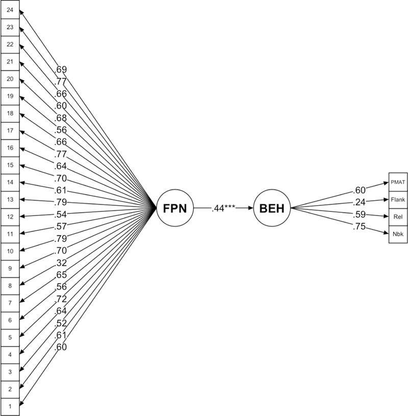
SEM path diagram for Model 4a from Example 4. Model 4a allows all parameters to be freely estimated (not constrained). Standardized factor loadings for the 24 parcels on the FPN latent variable, and the 4 cognitive measures on the behavioral (BEH) latent variable are shown. Standardized regression weight for FPN predicting BEH is shown. *p < .05, **p<.01, ***p<.001.

Table 4.

Regressions from Models 4a-e

Model	b*	SE	Z	R2
4a-AllFree	.44***	.02	8.91	.20
4b-NetworkFree	.38***	.01	8.09	.15
4c-BehavFree	.43***	.02	10.86	.19
4d-NoFree	.38***	.01	9.98	.14
4e-ZScoreComposite	.25***	.03	8.93	.07

“AllFree” – all factor loadings freely estimated; “NetworkFree” – factor loadings for FPN freely estimated, but factor loadings for BEH constrained; “BehavFree” – factor loadings for BEH freely estimated, but factor loadings for FPN constrained; “NoFree” – all factor loadings constrained.

^*p < .05

^**p<.01

^***p<.001.

One might be concerned that the increased R² values reported here are an artifact of overfitting, in the sense that perhaps R² increases because of sample specific variance. However, this is not actually the case, as the measurement model is separate from the structural latent variable model (e.g., relationships among latent variables), and it could be that R² is lower when the latent variables are freely estimated. That said, the freely estimated model will likely have a higher R² because the latent variables are more accurately measured (i.e., with less error). SEM models are also well-suited to choose models that will show generalizability to future samples. First, the larger sample size should minimize the influence the impact of sample specific variance, resulting in parameter estimates that are more stable and closer to population parameters. Second, choosing models based on fit indices like the Akaike Information Criterion (AIC) and Bayesian Information Criterion (BIC) are formally equivalent to cross-validation techniques such as k-fold cross-validation (AIC; Stone, 1977) and leave-one-out cross-validation (BIC; Shao, 1997). That is, selecting a model with the lowest AIC/BIC will minimize overfitting and result in generalizability to other samples. AIC/BIC values for the current analysis are shown in Table 3 and are lowest for Model 4a (the freely estimated model), which thus mitigates some of these overfitting concerns.

4.2.2.1c. Implications

There are a number of ways in which the enhanced predictive power of SEM can benefit cognitive neuroscientists. For instance, one of the most immediately fruitful applications of SEM is likely to be contextualizing individual differences at different “levels” of the brain. For example, a new study by Bolt et al. (2018) used SEM to ask how brain-behavior associations could change depending upon whether the level of analysis was at the individual ROI or the network level. They used a similar procedure as that shown here, such that parcellation algorithms were applied to get a set of parcels representative of a putative network (i.e., 24 parcels for the FPN network), and then selected one of those parcels as an a candidate ROI. They then probed the relationship between the latent network predicting behavior, and the ROI specifically predicting behavior. They repeated this process for different task contexts and behaviors: 1) FPN during the N-back predicting N-back accuracy, 2) FPN during the Relational task predicting relational accuracy, and 3) the cingulo-opercular network during the arithmetic task predicting arithmetic accuracy. For the first two of the three SEM analyses, they showed that the association between a ROI-level variable and behavioral variable disappeared after controlling for the network-level variable. However, the reverse was true for the last SEM such that the individual ROI-level variable predicted arithmetic accuracy over and above the latent network variable. They therefore conclude that brain-behavior associations can vary depending on the level of analysis (region of interest vs. network), and that both should be taken into consideration. The study by Bolt and colleagues (2018) is an interesting use case for SEM in the context of individual differences, and one that is likely to continue.

4.2.2.2. Example 5 – Convergent and Divergent Validity

4.2.2.2a. Brief Introduction and Analytic Approach

Since effectively interrogating individual differences questions hinges on psychometric considerations, many individual difference researchers are thus concerned with addressing questions surrounding validity. Researchers may want to ensure that an individual difference variable of interest correlates with other measures that it ought to correlate with, known as convergent validity. Similarly, divergent (or discriminant) validity ensures that an individual difference variable of interest does not correlate with measures it ought to not correlate with. For instance, HCP participants underwent 7 t-fMRI protocols, two of which were the N-back working memory task and a motor tapping task in which subjects were simply asked to tap their fingers, toes, or move their tongues in an effort to map motor regions (see Barch et al., 2013 for details on all 7 task protocols). The FPN would be expected to be particularly engaged during the N-back task (Cole et al., 2012); however, preferential engagement of the FPN would not be expected during the motor tapping task. Conversely, one would expect a network comprised of parcels from somatomotor regions to be especially activated by the motor task, but not especially activated (over and above other networks) during the N-back. Furthermore, between-subject variance captured by a latent FPN variable during the N-back should likely correlate with an out-of-scanner individual difference measure in the cognitive domain whereas the same FPN latent variable should not predict an out-of-scanner individual difference measure within the motor domain and vice versa. The purpose of Example 5 is to illustrate that convergent/divergent validity can be easily tested within the SEM framework.

Two SEMs were created, both taking the same structure: one latent FPN factor was defined by the same 24 FPN parcels measured during the N-back 2 back > 0 back contrast, and a new right hand (HAND) latent factor was defined by 20 parcels within the right hemisphere somatomotor cortex measured during the HCP motor task right hand > left hand contrast (i.e., the same parcellation algorithm was applied to the motor task for right hand, motor task for left hand, and then left was subtracted from right to generate the contrast). Then, regressions were set up such that the PMAT (an out-of-scanner individual difference measure of fluid intelligence that ought to relate to the N-back) was regressed on the latent FPN and latent HAND factors. Similarly, the Strength (age-adjusted) out-of-scanner individual difference measure of grip strength was regressed onto the latent FPN and HAND factors. We further ensured that the FPN and HAND latent factors would not correlate with each other, and that the PMAT and Strength individual difference measures would not correlate with each other. This was done to more precisely target convergent/divergent validity questions. Subjects with complete data were used, yielding a sample size of n = 1012. Model 5a was defined exactly as described above. In Model 5b, the only difference is that regression equations were defined, but constrained to be equal. Models 5a and 5b were then formally compared to test that the expected associations were significantly different from one another (i.e., that the FPN to PMAT association is significantly stronger than the FPN to HAND association, and vice versa). We hypothesized that the FPN (measured during the N-back) should predict the PMAT, but not Strength whereas the HAND network (measured during the motor task) should predict Strength, but not PMAT.

4.2.2.2b. Results

Indeed, Model 5a (freely estimated regression parameters) was significantly better than Model 5b (constrained regression parameters; Δχ²(4) = 758.89, p < .001), indicating divergent validity. Moreover, the regressions from Model 5a demonstrate that both the FPN and HAND latent networks exhibit good convergent validity (Figure 4). The PMAT was significantly predicted by FPN during the working memory task (b* = .25, z(1009) = 6.83, p < .001), but not by the HAND variable (b* = .01, z(1009) = .33, p = .739). Conversely, the Strength individual difference measure as significantly predicted by the HAND latent factor (b* = .10, z(1009) = 3.12, p = .002), but not by the FPN latent variable (b* = .02, z(1009) = .46, p = .650).

Figure 4.

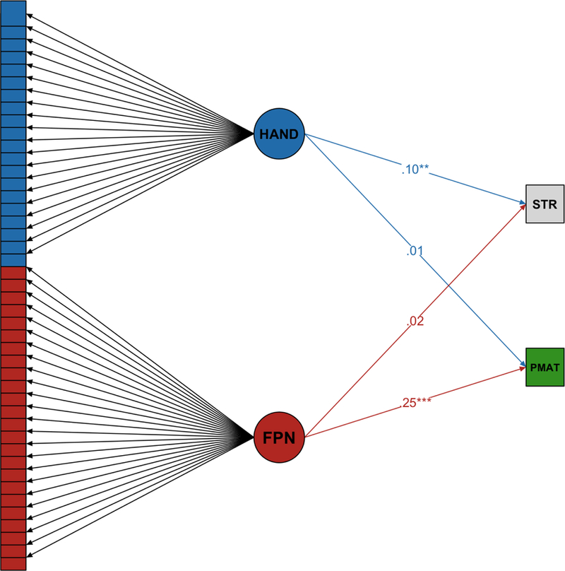
SEM path diagram for Example 5. Convergent validity: the HAND network (blue), as measured during the motor task, should predict grip strength (STR; gray). The FPN (red), as measured during the N-back, should predict fluid intelligence measured by Penn Progressive Matrices (PMAT; green). Divergent validity: HAND should not predict PMAT, and FPN should not predict STR. Standardized regression weights are shown. *p < .05, **p<.01, ***p<.001. Factor loadings can be found in Supplement 3.

4.2.2.2c. Implications

As more neuroimaging studies shift focus onto individual differences questions, being able to flexibly evaluate psychometric concerns, such as validity, will become increasingly important. The SEM framework can easily accommodate these types of questions. Though this example is only a very crude assessment of convergent/divergent validity, it is not difficult to imagine future studies including the FPN measured during the motor task and the HAND network measured during the N-back for a more thorough assessment of convergent and divergent validity (see Example 7 for a somewhat similar idea). Relatedly, researchers may want to harness SEM procedures to ensure than any in-scanner task adaptation does not compromise the integrity of the task (e.g., if a task is originally designed for schizophrenia patients, but adapted for use in bipolar disorder patients, one could use similar procedures to ensure that the task is still tapping the same underlying construct in the bipolar patients as it did in the schizophrenia patients).

4.2.2.3. Example 6 – Relative Influence of Task Contexts and Brain Networks

4.2.2.3a. Brief Introduction and Analytic Approach

A majority of the work in functional networks has been done in the resting state connectivity literature. If these networks are appropriate ways of carving the brain into meaningful sub-units, then the networks should still be functionally present in task activation contexts. However, it remains unclear if there is something jointly important about both the task and the network in predicting individual differences. In other words, a standard assumption – which is not often directly tested – is that specific brain networks are preferentially relevant for predicting individual differences that are most strongly tied to the functioning of that given network (e.g., the FPN network is preferentially important for predicting individual differences in working memory and executive control function). However, it could be the case that individual difference effects are not strongly tied to a particular network and could be accounted for by some more global measure of brain activity. Likewise, it could be the case that there is network-specific prediction of individual differences, but not selectively tied to a particular task context. The purpose of the following example, and the one after it, is to show how testing complex questions about brain-behavior relationships, like partitioning task and network contributions, can be addressed within an SEM framework.

Here, the same 24 indicators were defined to load onto a single FPN latent network variable during the N-back working memory task. Similarly, 39 indicators of the visual network, also measured during the N-back task, were added into the model, and were defined to load onto a single Visual (VIS) latent network variable. The VIS network was added here for comparison purposes, to test the assumption that activation of this network is less likely to reflect individual differences in working memory/executive control per se. To examine this question, we added a general latent factor called Task in which both the FPN and VIS indicators loaded, since activation was measured in both during the same N-back task. Importantly, the model was set up such that all correlations between these three latent variables (Task, FPN, and VIS) were constrained to equal zero. The resulting model is standardly termed a “bifactor” SEM. The Task latent factor reflects the variance shared across all indicators. The FPN latent factor reflects the remaining shared variance shared across all 24 FPN indicators, but critically, after controlling for the Task factor. Similarly, the VIS latent factor reflects the variance shared across all 39 visual indicators, after the variance shared across all indicators has been removed (because it is now captured by the Task latent factor). The same cognitive control behavioral latent factor (BEH) from Example 4 was used here as a primary outcome. Finally, we regressed the BEH latent variable on the FPN, VIS, and Task latent variables. Since all data were obtained during the N-back task, the sample size is the same as Examples 1–4 (n = 1019).

4.2.2.3b. Results

Primary results can be found in Figure 5. Individual differences in the FPN latent variable significantly predicted the cognitive control behavior (b* = .45, z(1015) = 8.56, p < .001). The VIS latent factor did not predict BEH (b* = .06, z(1015) = .32, p = .751). This is not surprising because after the variance shared across all parcels was extracted into the Task latent factor, there was very little unique variance left in the VIS network – factor loadings onto the VIS latent variable were very low (near zero and even some negatives; factor loadings for this analysis can be found in Supplement 4). That is, the shared variance amongst VIS parcels was also shared amongst FPN parcels, and was best accounted for by a more global Task latent variable. Interestingly, the Task latent factor did significantly predict BEH (b* = .13, z(1015) = 3.46, p = .001). This indicates that both the FPN brain network and, possibly the N-back task context itself, are both important elements of individual difference. Overall fit estimates were within the range of the other previous examples: CFI - .75, TLI - .73, RMSEA - .08, SRMR - .07.

Figure 5.

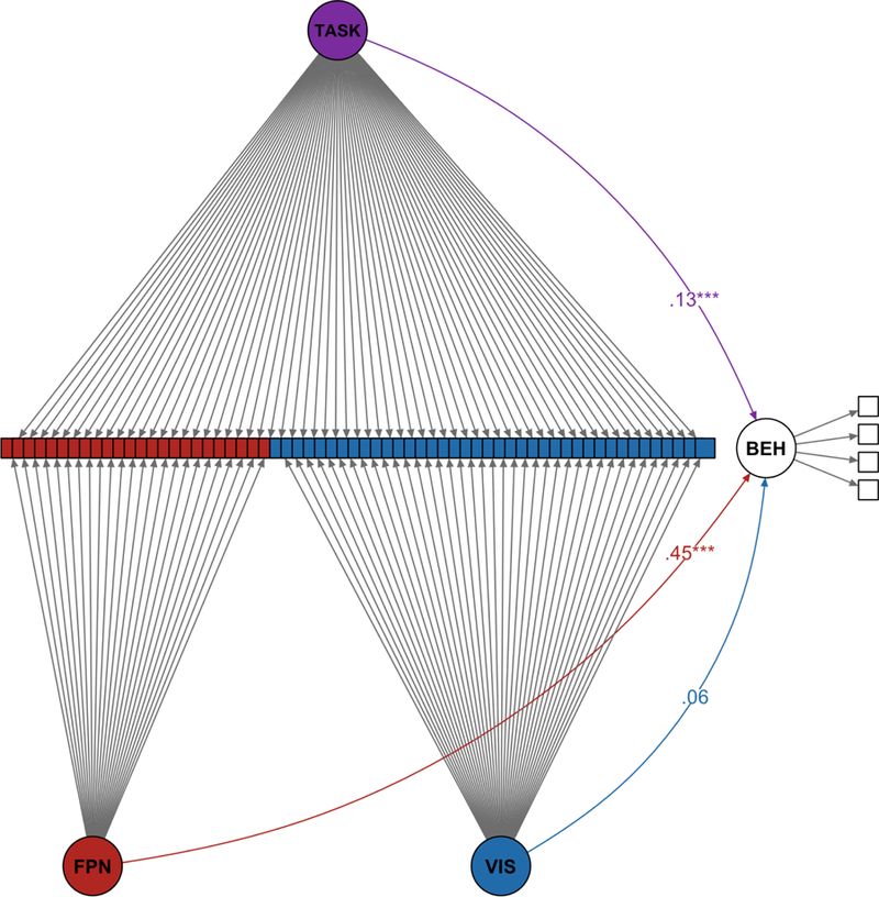
SEM path diagram for Example 6. Bifactor SEM such that the TASK (purple) latent variable reflects the between-subjects variance across all parcels, after controlling for respective brain networks. FPN (red) is the between-subject variance across 24 FPN parcels, after controlling for TASK. Visual (VIS; blue) is the between-subject variance across 39 visual parcels, after controlling for TASK. Standardized regression weights from the bifactor SEM predicting the latent behavioral (BEH) variable are shown. *p < .05, **p<.01, ***p<.001. Factor loadings can be found in Supplement 4.

4.2.2.3c. Implications

This example has, thus far, been the most complex SEM presented, yet highlights the ways in which researchers can test nuanced hypotheses. Importantly, we simultaneously accounted for the task state and neural activation inherent in t-fMRI data, and partitioned the variance accordingly. In addition to expanding this to include more networks and tasks, future studies could also use this approach for testing hypotheses regarding the importance of task-related and brain-related individual differences dimensions. For example, one might hypothesize that individual differences in sensorimotor behaviors may be best fit by a global activity factor, whereas more specific brain networks and/or task activation contexts may better capture individual differences in more classically “higher order” cognitive behaviors.

4.2.2.4. Example 7 – Are Brain Networks Independent of Task Context?

4.2.2.4a. Brief Introduction and Analytic Approach

In the previous example, two brain networks obtained during the same task activation context (the N-back) were interrogated in order to determine if each brain network, and the task network, were meaningful dimensions of individual difference. In this final example, we take a slightly different approach to ask a very related question. Though networks can be defined in various task contexts (or resting state), it remains unclear if brain networks are particularly useful individual difference dimensions if and only if measured during a particular task (e.g., the FPN during the N-back), or if the network itself, independent of task context, is the crucial individual difference dimension. Importantly, if a brain network is thought to be the vital individual difference dimension in a task-independent manner, then any parcel within that network, in any task context, would be considered multiple measurements of the same underlying construct. Put differently, if the FPN acts in a task-independent manner, then one could obtain 24 measurements of the network (one per parcel) during the N-back task and an additional 24 measurements of the network during another context, such as the motor task, thus effectively doubling the number of indicators and supposedly better capturing the “true” FPN network. In this scenario, the latent FPN factor measured during the N-back task should share a lot of variance with the latent FPN factor measured during the motor task, and even converge to form a second-order latent FPN factor that would be considered a “global” FPN factor. Yet if the FPN does not act in a task-independent manner, then there would be little variance shared between the FPN networks from the two task contexts, and the second-order latent variable would not reflect a meaningful individual difference dimension.

We defined an SEM accordingly: a latent FPN network variable from the N-back, a latent FPN network variable from the motor task, and then a second-order “global” FPN latent factor. Additionally, we include the same cognitive control behavioral composite (BEH) seen in Examples 4 and 6. Regression equations were specified in order to determine which of the three latent factors best predict behavior. No additional constraints were placed. Since this model includes the motor task, n = 1012.

4.2.2.4b. Results

The hypothesis that the FPN acts in a task-independent manner was not supported by the data (Figure 6). Specifically, the N-back working memory FPN did not load at all onto the global FPN factor, and the global FPN factor was entirely comprised of variance from the FPN motor factor. Neither the global FPN nor FPN motor factors significantly predicted behavior, whereas the FPN working memory factor did significantly predict BEH (b* = .45, z(1008) = 8.59, p < .001). Though not shown here, we conducted a follow-up analysis in which a similar model was defined, yet the second-order global factor was not fit (this was done to make sure our results were not skewed simply due to fitting the second-order variable). The FPN measured during the motor task still did not predict BEH in this follow-up procedure. Overall fit estimates for Model 7 were within the range of the other previous examples: CFI - .74, TLI - .73, RMSEA - .08, SRMR - .06. Taken together, these findings suggest that the FPN is a meaningful source of cognitive individual difference, but potentially only when examined through the lens of a specific task context that is thought to be dependent on the functions supported by the FPN.

Figure 6.

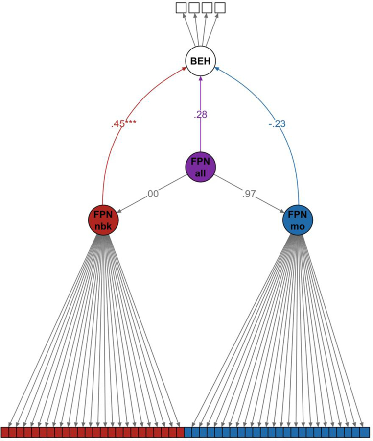
SEM path diagram for Example 7. The FPN as measured during the N-back (red) and the FPN as measured during the motor task (blue) are shown. A second-order global factor (FPN all; purple) was fit to capture the shared variance between FPN in the N-back and FPN in the motor task. Standardized factor loadings are shown in gray. Standardized regression weights are shown for each of the three latent FPN variables predicting the latent behavioral (BEH) variable. *p < .05, **p<.01, ***p<.001. Factor loadings can be found in Supplement 5.

4.2.2.4c. Implications

Examples 6 and 7 were primarily included to illustrate that very complex questions surrounding individual differences in brain networks can be examined from a latent variable perspective. In particular, Examples 6 and 7 take slightly different, but related approaches to better understanding the circumstances around which a brain network might capture meaningful between-subject variance. Future studies could expand upon this in a multitude of ways. For example, one could examine the relative stability of a brain network across a variety of task contexts. Or perhaps examine whether a brain network is a better or worse dimension of individual differences across various behavioral sub-domains (e.g., rather than just examining executive control, one could assess how a network might change across proactive and reactive control states; Braver et al., 2010; Braver, 2012). In all, these are just some of the ways that latent variable approaches like SEM can be harnessed for nuanced hypothesis testing regarding the neural underpinnings of cognitive individual difference.

4.3. Other SEM Uses

The above seven examples were presented to demonstrate how SEM could be applied in standard t-fMRI settings. However, these are not the only ways in which SEM can be implemented. Below is a brief description of other use cases not touched upon in the above examples.

The brain is a dynamic organ that changes over time. SEM is well equipped to handle longitudinal data, allowing researchers to interrogate how brain-behavior relationships change given repeated measures data. A SEM model could be used in this way by incorporating autoregressive effects and cross-lagged effects (construct at time 1 can predict a different construct at time 2) or contemporaneous effects (a construct predicting a different construct, but not lagged in time). Relevant concrete t-fMRI questions that could be addressed with such an approach include testing if individual differences are stable across multiple waves of data collection (on par with the idea of test-retest reliability), or even over the course of development or age-related declines. For more on the longitudinal applications of SEM, see Little, 2013.

Seeing as t-fMRI is currently undergoing a “big data” revolution of sorts, it is noteworthy that SEM frameworks can ease some of the challenges associated with analyzing these types of datasets. Depending on the size of the dataset, one might have the unique opportunity to replicate their findings. For instance, the Adolescent Brain Cognitive Development study (see section 3.2) will be assessing over 10,000 children. Researchers may want to use the SEM framework to demonstrate brain-behavior associations on 5,000 children first, and then test the same model on the remaining 5,000 children in hopes of reproducing the brain-behavior relationships, while avoiding overfitting concerns. One could use a similar approach for completely avoiding the non-independence error that plagues t-fMRI correlational studies (Kriegeskorte et al., 2009; Vul et al., 2009). By dividing the dataset in half, one could use the standard procedure of first defining relevant voxel clusters via demonstration of a correlation to an individual differences behavioral measure. The measurement model would then be defined in terms of latent variables (across the voxel clusters or regions). But then validation and hypothesis testing of this model would be in the held-out data (i.e., keeping constant the loading factors). This would be a prime example of complementary hypothesis generating and hypothesis testing studies. Finally, SEM can easily accommodate covariates that could potentially impact big data projects (Smith and Nichols, 2018). For example, data can be collected on different types of scanners at different locations. If the data are coded accordingly, then study site or scanner type (categorical variables) could be entered into the SEM as covariates. In such cases, the observed covariate is regressed onto the latent variable (the arrow switches direction), since the interpretation would be that some of the variance in the latent factor is accounted for by the covariate. Similar approaches could be taken for potentially psychologically more interesting covariates as well, such as gender, age, and ethnicity.

5. Conclusions

Understanding the intricacies of brain-behavior relationships requires more flexible analytic methods beyond correlations; likewise, interpreting these individual difference findings requires in-depth knowledge of the psychometric qualities of both behavioral assessments and t-fMRI measurements. Concepts and methodological tools from the field of psychometrics, such as latent variable modeling (including SEM), can help with both points. Latent variable approaches provide researchers with unprecedented opportunities to formally and rigorously take a hypothesis testing perspective to questions surrounding the neural underpinnings of cognitive individual difference. Application of such analytic methods allows cognitive neuroscientists to incorporate known sources of between-subject variance (e.g., task contexts, task performance, brain networks, non-task related individual differences, etc.) into parsimonious, theoretically-specified models, ultimately yielding a more holistic understanding of brain-behavior relationships. We hope that this review will encourage the greater integration of such approaches as a mean to enhance the rigor and scope of individual differences questions being addressed within cognitive neuroscience research.

Highlights.

• Understanding individual differences requires consideration of psychometrics

• Psychometric frameworks are not often used in fMRI due to power/sample size issues

• Latent variable models are flexible and can address psychometric concerns

• Individual differences in fMRI can be better understood via latent variable models

• Recent big data fMRI projects provide opportunity to harness latent variable models