Deep learning for automated segmentation of pelvic muscles, fat and bone from CT studies for body composition assessment

Abstract

Objective:

To develop a deep convolutional neural network (CNN) to automatically segment an axial CT image of the pelvis for body composition measures. We hypothesized that a deep CNN approach would achieve high accuracy when compared to manual segmentations as the reference standard.

Material and Methods:

We manually segmented 200 axial CT images at the supraacetabular level in 200 subjects, labeling background, subcutaneous adipose tissue (SAT), muscle, inter-muscular adipose tissue (IMAT), bone and miscellaneous intra-pelvic content. The dataset was randomly divided into training (180/200) and test (20/200) datasets. Data augmentation was utilized to enlarge the training dataset and all images underwent preprocessing with histogram equalization. Our model was trained for 50 epochs using the U-Net architecture with batch size of 8, learning rate of 0.0001, Adadelta optimizer and a dropout of 0.20. The Dice (F1) score was used to assess similarity between the manual segmentations and the CNN predicted segmentations.

Results:

The CNN model with data augmentation of N=3,000 achieved accurate segmentation of body composition for all classes. The Dice scores were as follows: background (1.00), miscellaneous intra-pelvic content (0.98), SAT (0.97), muscle (0.95), IMAT (0.91) and bone (0.92). Mean time to automatically segment one CT image was 0.07 seconds (GPU) and 2.51 seconds (CPU).

Conclusions:

Our CNN based model enables accurate automated segmentation of multiple tissues on pelvic CT images, with promising implications for body composition studies.

INTRODUCTION

The gluteal, piriformis and iliopsoas muscles play an important role in providing stability and mobility of hips and lower extremities. Atrophy and fatty infiltration of pelvic muscles are associated with pathological conditions such as hip osteoarthritis, neuromuscular disorders and iatrogenic injury during hip replacement surgery [1–4]. Moreover, this process can be seen as part of a more generalized age-related loss of muscle volume and fatty infiltration known as sarcopenia [5–8]. Body composition (amount and distribution of adipose tissue and muscle in the human body) and sarcopenia are increasingly relevant as predictors of overall health, and has been associated with osteoporosis [9] and poor outcomes after surgery, trauma and cancer [10–13].

Cross-sectional imaging techniques, such as computed tomography (CT) and magnetic resonance imaging (MRI), are part of the clinical workup for many diseases and enable accurate measurement of body composition [11]. Accurate segmentation of different tissues plays a key role in reliably measuring body composition, which is currently done using time-consuming manual or semi-automated methods. Consequently, the use of valuable body composition parameters for clinical management is limited, underlining the need for reliable automated segmentation methods. Recently, fully automated segmentation methods using deep learning techniques have been published for automatic segmentation of abdominal CTs at a lumbar level [14–16] and MRI at the mid-thigh level [17]. However, no prior studies have evaluated automated systems to measure muscle mass at the pelvis. The purpose of our study was to develop a deep convolutional neural network (CNN) to automatically segment an axial CT image at a standardized pelvic level for body composition measures. We hypothesized that the application of a U-net CNN would achieve high accuracy as compared to the reference standard of manual segmentation.

MATERIALS AND METHODS

Our study was IRB-approved and complied with Health Insurance Portability and Accountability Act (HIPAA) guidelines with exemption status for individual informed consent.

Dataset

A dataset of 200 patients who underwent an abdominal CT examination between January 2017 and December 2019 was collected retrospectively. The abdominal CTs were performed using multi-detector CT scanners (General Electric, Waukesha, WI, USA) at our institution. Patients were scanned in supine position, head first and with arms over the head. The field of view was adapted to the patient’s body habitus.

Ground truth labeling (manual segmentation)

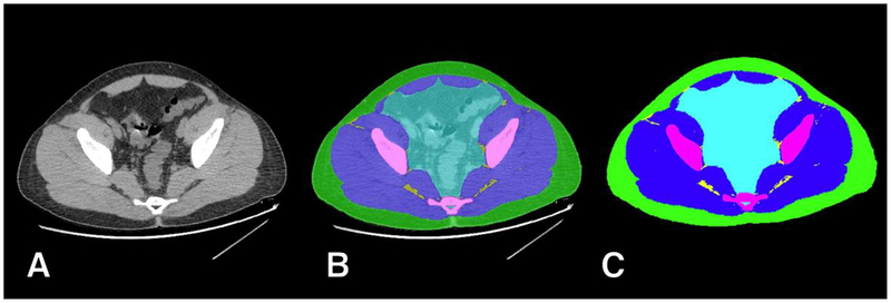
In order to evaluate pelvic muscle mass, we selected a standardized single axial image immediately cranial to the acetabular roof. This supra-acetabular level was chosen as it is easily recognizable and contains substantial muscle mass that includes the main hip stabilizers (gluteal, piriformis and iliopsoas muscles), having been used in previous studies of pelvic body composition [1, 2, 18, 19]. Manual segmentation was performed using manual and semi-automated thresholding using the Osirix DICOM viewer (version 6.5.2, www.osirix-viewer.com/index.html) by a single operator with 9 years of experience, with images and segmentations audited by a second investigator with 22 years of experience. As shown in Figure 1, examinations were segmented manually into six classes, each with a unique color: (1) background pixels (external to the pelvis; black), (2) subcutaneous adipose tissue (SAT; green); (3) muscle (blue); (4) inter-muscular adipose tissue (IMAT; yellow); (5) bone (magenta); (6) miscellaneous intra-pelvic content (e.g. bowel, vessels and visceral adipose tissue; cyan). Previously used thresholds in Hounsfield Units (HU) were applied: −29 to +150 HU for muscle and −190 to −30 HU for SAT [20]. For IMAT, we first performed a morphological erosion with a structuring element of radius 3 pixels on the muscle region to remove artifacts at the edges of segmentation. This was followed by thresholding pixels in the −190 to −30 HU range within the eroded muscle region. The segmented images were stored as anonymized Tag Image File Format (TIFF), with masks being 8-bit RGB and corresponding CT images being 8-bit single-channel grayscale. All images had dimensions of 512×512 pixels.

Figure 1.

Example of manual ground truth segmentation. The axial CT image at pelvic level (A) is manually segmented into multiple tissues (B) resulting in a mask (C) with 6 classes: background (black); subcutaneous adipose tissue (SAT, green); muscle (blue); inter-muscular adipose tissue (IMAT, yellow); bone (magenta); and miscellaneous intra-pelvic content (cyan).

Model

Preprocessing

The dataset was randomly divided into training (180/200, 90%) and test (20/200, 10%) datasets, ensuring training and test datasets were fully segregated with no overlap. Manually segmented IMAT labels (yellow) in masks of the training dataset were converted to the muscle class (blue). As discussed below, we aimed to first train a model that would reliably predict the location of muscle pixels on a slice. Then, using standard HU thresholding after the CNN prediction, we proceeded to select IMAT pixels within the predicted muscle region. Contrast limited adaptive histogram equalization (CLAHE) was performed on all grayscale images followed by image augmentation of the training dataset. Image augmentation was performed on grayscale and ground truth mask pairs to enlarge the training dataset by applying random rotation, flipping, cropping and scaling (N=500, 1000, 2000, 3000). In addition, 50% of augmented grayscale images were randomly added with Poisson noise to further increase variability and improve generalizability.

Training and testing

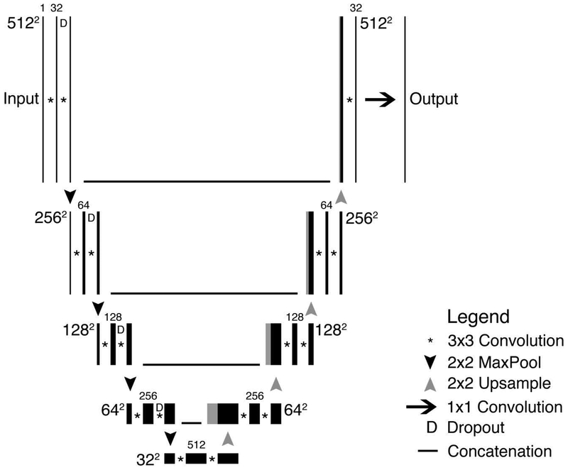
We used the U-Net convolutional neural network (CNN) architecture [21], which was previously developed by others to segment medical images. A schematic of the used U-Net architecture is depicted in Figure 2. Briefly, images with 512×512 pixels were input in our U-Net structure that consisted of five layers with four down-sampling steps resulting in a 32×32×512 representation followed by four up-sampling steps. Each step consisted of two successive 3×3 padded convolutions, and in the down-sizing steps, a dropout of 0.20 was applied. This was followed by a rectified linear unit (ReLU) activation function and a max-pooling operation with a 2×2 pixel kernel size. The up-sampling operations were performed using a 2×2 transposed convolution followed by a 3×3 filter size convolution after which the output concatenates with the corresponding decoding step. The final layer consisted of a 1×1 convolution followed by a sigmoid function, resulting in an output prediction score for each class.

Figure 2.

Schematic of U-Net architecture used to predict segmentations. As can be seen in the figure, the processing map resembles a “U”.

Our model was written and trained in Python 3.7 (Python Software Foundation, Beaverton, Oregon) using the Keras library (v2.2.4, https://keras.io) with Tensorflow 1.13.1 (Google, Mountain View, California) [22]. For training, optimal parameters were experimentally determined. The training dataset (N=180) was corrected for differences by weighting class prevalence. A batch size of 8 was used with a learning rate of 0.0001, Adadelta optimizer, dropout of 0.20 and 50 epochs. Training was performed on a multi-GPU (4x NVIDIA Titan Xp units) Linux workstation running the Ubuntu 14.04 operating system.

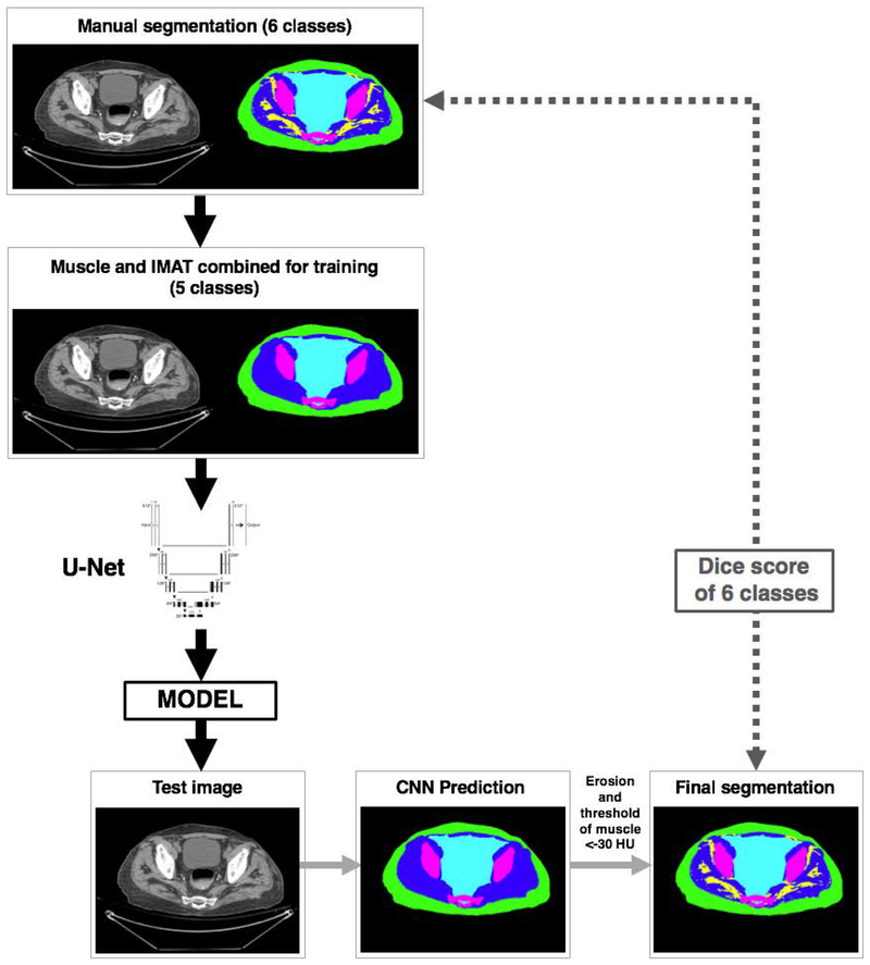
Testing followed the workflow described in Figure 3. Grayscale images from the test dataset (N=20) were exposed to the trained model to produce predictions in 5 classes (background, SAT, muscle, bone and miscellaneous). As described above, a morphological erosion procedure of the muscle predicted region was followed by thresholding of pixels with values < −30HU being classified as IMAT. The final segmentation was then tested by comparing its predictions of 6 classes to the manually segmented test dataset.

Figure 3.

Schematic of the segmentation and analysis workflow.

Statistical Analysis

Descriptive statistics were reported in terms of percentages and means ± standard deviations (SD). The Dice (F1) score was used to assess similarity between the manual segmentations and the CNN predicted segmentations [23]. A Dice score of 1.00 is a perfect similarity. For a ground truth segmentation S_g and a predicted segmentation S_p the Dice score can be calculated as:

$$\text{Dice score}=\frac{2\left|{\text{S}}_{\text{g}}\cap {\text{S}}_{\text{p}}\right|}{\left|{\text{S}}_{\text{g}}\right|+\left|{\text{S}}_{\text{p}}\right|}$$

RESULTS

A total of 200 CT images were collected from 200 patients who underwent an abdominal CT examination between January 2017 and December 2019. The included patients had a mean age of 49.9±17.7 years and consisted of 102/200 (51%) males. The patients had a mean weight of 82.3±19.2 kg and mean BMI of 29.0±6.1 kg/m².

Of the included examinations, 106/200 (53%) were non-enhanced with intravenous contrast, 67/200 (33%) had intravenous contrast enhancement only, 15/200 (8%) had only oral contrast, and 12/200 (6%) had both intravenous and oral contrast. CT imaging parameters as taken from the Digital Imaging and Communications in Medicine (DICOM) headers are depicted in Table 1. Manual segmentations were accomplished in approximately 15 minutes per image.

Table 1.

CT imaging parameters of 200 images used in the study.

	Value
Device a
Lightspeed VCT, GE	154 (77%)
Revolution CT, GE	42 (21%)
Discovery CT750, GE	4 (2%)
CT tube current (mA) b	343.1±124.3
Peak tube voltage (kVp) a
100	4 (2.0%)
120	159 (79.5%)
140	37 (18.5%)
Section thickness (mm) a
2.5 mm	200 (100%)

^aData are number (percentage)

^bData are mean ± standard deviation

Augmentation provided incremental benefit to segmentation accuracy beyond N=1,000. Given our focus on accuracy of soft tissue boundaries (i.e., muscle, fat, intra-pelvic content) we used the model generated from N=3,000 augmentations (Table 2). Training for 50 epochs took approximately 1.11 hours. At testing, our model produced accurate segmentations of body composition for all classes. The Dice scores were as follows: background (1.00), miscellaneous intra-pelvic content (0.98), SAT (0.97), muscle (0.95), IMAT (0.91), and bone (0.92). On our multi-GPU workstation, each automated segmentation was accomplished in 0.07 ± 0.23 seconds. On an older 8-core workstation (Apple Mac Pro 2009) using CPU only, each segmentation was performed in 2.51 ± 0.22 seconds.

Table 2.

Effect of data augmentation on tissue Dice scores.

Augmentation (N)	Background	Muscle	SAT	Bone	Miscellaneous
500	0.99	0.93	0.95	0.91	0.95
1,000	1.00	0.96	0.97	0.93	0.97
2,000	0.99	0.96	0.96	0.93	0.97
3,000*	1.00	0.96	0.97	0.92	0.98
4,000	1.00	0.96	0.97	0.92	0.97

SAT, subcutaneous adipose tissue. Miscellaneous class include all non-muscle intra-pelvic content.

^*, model with highest Dice scores for soft tissue classes used for final experiments.

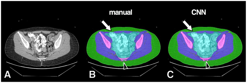
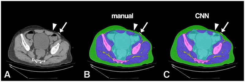
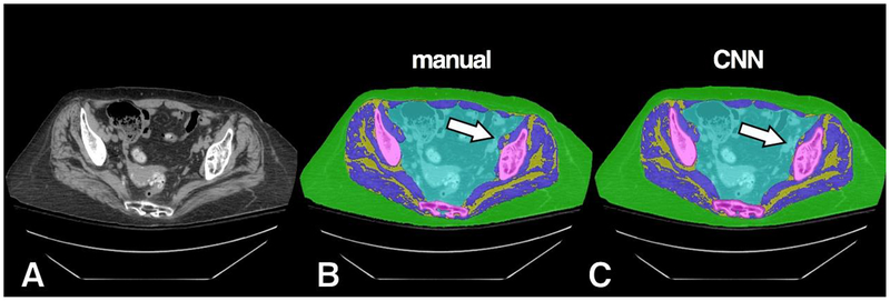
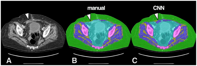
Figures 4–8 show examples of automatic prediction of the different segmented classes with high accuracy level. Although overall accuracy was high throughout the test dataset, some prediction errors were found in challenging areas, such as interfaces between muscles and pelvic content (Figure 5) and along anterior abdominal wall muscles (Figures 7, 8).

Figure 4.

Example of high accuracy segmentation. Original grayscale image (A), manual segmentation (B) and CNN segmentation (C). Minor CNN prediction overestimations noted at anterior muscle/subcutaneous interface (arrow) and surrounding distal sacral cortex (arrowhead). Bowel contrast material and cross section of scanner bed were consistently classified correctly by the CNN model as intra-pelvic content and background, respectively.

Figure 8.

Example of misclassification of soft tissue density in the left anterior abdominal wall. Original grayscale image (A), manual segmentation (B) and CNN automated segmentation (C). A small area of CNN misclassification is seen along the left rectus abdominis muscle (arrowhead). A metallic density on the anterior skin was correctly ignored by the model as background (arrow).

Figure 5.

Example of high accuracy segmentation with minor misclassification on a subject with more prominent IMAT. Original grayscale image (A), manual segmentation (B) and CNN segmentation (C). A small area of CNN misclassification is seen along the left iliopsoas muscle (arrow), which was predicted instead as intra-pelvic content.

Figure 7.

Example of misclassification of soft tissue density in the right anterior abdominal wall. Original grayscale image (A), manual segmentation (B) and CNN segmentation (C). An area of soft tissue density (arrowhead), likely related to scarring from prior surgery, was misclassified by the CNN model as muscle.

DISCUSSION

In this study we show that a deep CNN model is able to accurately and automatically segment pelvic compartments relevant to body composition on clinical CT scans of the abdomen/pelvis. Our results are comparable to prior studies using automated methods to measure muscle mass in other anatomic regions, such as the abdomen at the third (L3) and fourth (L4) lumbar vertebrae, and the mid-thigh [14–16]. Importantly, our results are novel in showing the feasibility of this method to obtain reliable muscle mass measures in the pelvis, which has important implications for studies of muscle wasting and sarcopenia. Further, we introduce a novel workflow for automated segmentation of IMAT, whereby pixels within a CNN-predicted muscle region undergo standard HU thresholding.

There is growing interest in oncology on the prognostic value of muscle wasting, sarcopenia and body composition. Studies in cancer patients showed that muscle and adipose tissue distribution are risk factors for clinical outcomes such as post-operative complications, chemotherapy-related toxicity, and overall survival [11,24,25]. Further, sarcopenia has been associated with a decreased bone mineral density [9] and unfavorable outcomes (e.g. prolonged hospitalization and increased 1-year mortality) after major surgery and trauma [10,12,13]. Currently, one of the major drawbacks for broader implementation of body composition and sarcopenia measures in routine clinical care is the necessity of manually segmenting images.

Accurate manual segmentation is a tedious task requiring up to 20–30 min per slice [26]. To overcome this practical limitation, automatic segmentation techniques have been described in recent years. These techniques include the use of atlas-based methods for the purpose of segmenting skeletal muscles [27] and use of threshold-based methods for automatic segmentation of adipose tissue [28–30] at abdominal levels. The abdominal and pelvic anatomical variations pose a considerable challenge for these methods, potentially requiring manual editing of segmentations. To address this limitation, we examined – after manual slice selection – a fully automated CNN-based method, which enabled complete segmentation of all tissues of interest in about 2.5 seconds per patient with a high level of accuracy.

Currently, body composition and muscle mass derived from abdominal CT scans are mostly evaluated at the level of L3 and L4. For the purpose of our study, we focused on a standard pelvic level since fatty infiltration and atrophy of pelvic musculature is found to be associated with hip osteoarthritis, neuromuscular disorders such as limb-girdle muscular dystrophies and Miyoshi distal myopathy, and post-polio syndrome [1–3,31]. Although total body muscle volume correlates strongly with an axial level 5 centimeters above the L4–L5 level [32], measurements of sarcopenia at L3 have also shown value and can be significantly different from other vertebral levels [33]. Moreover, muscle mass at the pelvic girdle is larger compared to muscle mass at L3 and L4 [33] and is functionally an important compartment in regards to trunk and lower extremity mobility.

The results from our segmentation of different pelvic compartments showed an accuracy comparable or better to deep learning methodologies performed at the L3 level [14–16]. For example, Weston et al. found Dice scores of 0.93, 0.88, and 0.95 at the L3 level for SAT, muscle, and bone, respectively [14]. Lee et al. found a Dice score of 0.93 for muscle [15] and Wang et al. found a Dice score of 0.97 for SAT at the L3 level [16]. Although the results of our model are promising regarding accuracy and short analysis time per image, some over- and underestimations were seen. These errors occurred most commonly at the borders of the pelvic cavity and muscles: in some cases, our model was challenged by the margins between abdominal muscles and the adjacent bladder or bowel structures especially in patients with low amounts of visceral adipose tissue. These anomalies are in line with the results of Weston et al., who showed that the automatic segmentation of visceral adipose tissue had a larger standard deviation compared to other segmented compartments [14]. Nevertheless, the observed errors had no substantial effect on the overall accuracy of the model.

Strengths of our study include demonstration of highly accurate automated segmentations of pelvic soft tissues derived from a relatively small training dataset of manual segmentations (N=180). This feature has important implications for development of future models in body composition, given the labor-intensive nature and expertise required for generating such ground truth datasets. Another innovation of our study was the successful implementation of IMAT segmentation using thresholding of pixels located within the model-predicted muscle region. This simple but robust technique has not been previously described and yielded excellent Dice scores, suggesting this approach may be a strong candidate for similar tasks in other anatomic areas (e.g., muscle mass of thigh or at L4, T12). Given the potential metabolic implications of high amounts of IMAT and its link to sarcopenia, having accurate measures of this particular parameter represent an important technical contribution.

Limitations of our study include the model being trained using a single standardized slice at the pelvis. Likely, evaluation of multiple levels in the pelvis could provide further detail on muscle mass. However, this addition would require dedicated models to preserve high accuracy, increasing the computational cost at the prediction stage. Our model was trained and tested on CT at the level of acetabular roof, and its accuracy at pelvic levels more caudal or cranial is therefore not clear. Although our model was trained using a dataset with varied characteristics (e.g., gender, with and without oral/intravenous contrast, varied BMIs), data was from a single institution and variations in patient population, equipment and scanning technique may affect accuracy. A potential limitation may include our cohort trending towards overweight BMIs, with possible variations in accuracy for subjects with very low BMI. Although a division of datasets into 90% for training and 10% for testing is commonly used in the literature [14], testing our model on larger datasets may show variations in performance that were not present when using our limited test dataset of randomly selected patients (20/200, 10%). Finally, the clinical value of pelvic muscle mass measures should be evaluated in prospective clinical studies to determine their role in predicting outcome and prognosis in different oncology and non-oncology conditions. This clinical validation is important when subjects may present ascites (e.g. liver cirrhosis, ovarian cancer) or hemoperitoneum (e.g., major trauma), as such variations may limit accurate delineation of intra-pelvic content and adjacent muscles.

In conclusion, we showed that our CNN-based model enables accurate automated segmentation for body composition on abdominal CTs at the pelvic level. This model can generate highly accurate body composition measures within seconds, which has promising implications for clinical risk stratification and large-scale research workflows. Further testing on a larger patient population scanned on a wider variety of equipment is needed to validate these highly promising preliminary results.

Figure 6.

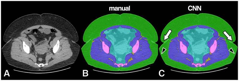
Example of high accuracy segmentation on a subject with prominent SAT. Original grayscale image (A), manual segmentation (B) and CNN segmentation (C). The CNN model successfully resolved prediction in boundaries such as skin folds (arrows) and field-of-view cut-off (arrowheads).

REFERENCES

- 1.Grimaldi A, Richardson C, Stanton W, Durbridge G, Donnelly W, Hides J. The association between degenerative hip joint pathology and size of the gluteus medius, gluteus minimus and piriformis muscles. Manual Therapy. 2009;14:605–10. [DOI] [PubMed] [Google Scholar]
- 2.ten Dam L, van der Kooi AJ, Rövekamp F, Linssen WHJP, de Visser M. Comparing clinical data and muscle imaging of DYSF and ANO5 related muscular dystrophies. Neuromuscular Disorders. 2014;24:1097–102. [DOI] [PubMed] [Google Scholar]
- 3.Woodley SJ, Nicholson HD, Livingstone V, Doyle TC, Meikle GR, Macintosh JE, et al. Lateral hip pain: findings from magnetic resonance imaging and clinical examination. The Journal of orthopaedic and sports physical therapy. 2008;38:313–28. [DOI] [PubMed] [Google Scholar]
- 4.Pfirrmann CWA, Notzli HP, Dora C, Hodler J, Zanetti M. Abductor tendons and muscles assessed at MR imaging after total hip arthroplasty in asymptomatic and symptomatic patients. Radiology. 2005;235:969–76. [DOI] [PubMed] [Google Scholar]
- 5.Ikezoe T, Mori N, Nakamura M, Ichihashi N. Atrophy of the lower limbs in elderly women: is it related to walking ability? European journal of applied physiology. 2011;111:989–95. [DOI] [PubMed] [Google Scholar]
- 6.Kiyoshige Y, Watanabe E. Fatty degeneration of gluteus minimus muscle as a predictor of falls. Archives of Gerontology and Geriatrics. 2015;60:59–61. [DOI] [PubMed] [Google Scholar]
- 7.Marcus RL, Addison O, Kidde JP, Dibble LE, Lastayo PC. Skeletal muscle fat infiltration: impact of age, inactivity, and exercise. The journal of nutrition, health & aging. 2010;14:362–6. [DOI] [PMC free article] [PubMed] [Google Scholar]
- 8.Visser M, Goodpaster BH, Kritchevsky SB, Newman AB, Nevitt M, Rubin SM, et al. Muscle mass, muscle strength, and muscle fat infiltration as predictors of incident mobility limitations in well-functioning older persons. The journals of gerontology Series A, Biological sciences and medical sciences. 2005;60:324–33. [DOI] [PubMed] [Google Scholar]
- 9.Oliveira A, Vaz C. The role of sarcopenia in the risk of osteoporotic hip fracture. Clinical rheumatology. 2015;34:1673–80. [DOI] [PubMed] [Google Scholar]
- 10.Chang C-D, Wu JS, Mhuircheartaigh JN, Hochman MG, Rodriguez EK, Appleton PT, et al. Effect of sarcopenia on clinical and surgical outcome in elderly patients with proximal femur fractures. Skeletal radiology. 2018;47:771–7. [DOI] [PubMed] [Google Scholar]
- 11.Brown JC, Cespedes Feliciano EM, Caan BJ. The evolution of body composition in oncology-epidemiology, clinical trials, and the future of patient care: facts and numbers. Journal of Cachexia, Sarcopenia and Muscle. 2018;9:1200–8. [DOI] [PMC free article] [PubMed] [Google Scholar]
- 12.Yoo T, Lo WD, Evans DC. Computed tomography measured psoas density predicts outcomes in trauma. Surgery. 2017;162:377–84. [DOI] [PMC free article] [PubMed] [Google Scholar]
- 13.Janssen I, Heymsfield SB, Ross R. Low relative skeletal muscle mass (sarcopenia) in older persons is associated with functional impairment and physical disability. Journal of the American Geriatrics Society. 2002;50:889–96. [DOI] [PubMed] [Google Scholar]
- 14.Weston AD, Korfiatis P, Kline TL, Philbrick KA, Kostandy P, Sakinis T, et al. Automated Abdominal Segmentation of CT Scans for Body Composition Analysis Using Deep Learning. Radiology. 2019;290:669–79. [DOI] [PubMed] [Google Scholar]
- 15.Wang Y, Qiu Y, Thai T, Moore K, Liu H, Zheng B. A two-step convolutional neural network based computer-aided detection scheme for automatically segmenting adipose tissue volume depicting on CT images. Computer Methods and Programs in Biomedicine. 2017;144:97–104. [DOI] [PMC free article] [PubMed] [Google Scholar]
- 16.Lee H, Troschel FM, Tajmir S, Fuchs G, Mario J, Fintelmann FJ, et al. Pixel-Level Deep Segmentation: Artificial Intelligence Quantifies Muscle on Computed Tomography for Body Morphometric Analysis. 2017; [DOI] [PMC free article] [PubMed] [Google Scholar]
- 17.Yang YX, Chong MS, Tay L, Yew S, Yeo A, Tan CH. Automated assessment of thigh composition using machine learning for Dixon magnetic resonance images. Magma (New York, NY). 2016;29:723–31. [DOI] [PubMed] [Google Scholar]
- 18.Momose T, Inaba Y, Choe H, Kobayashi N, Tezuka T, Saito T. CT-based analysis of muscle volume and degeneration of gluteus medius in patients with unilateral hip osteoarthritis. BMC musculoskeletal disorders. 2017;18:457. [DOI] [PMC free article] [PubMed] [Google Scholar]
- 19.Uemura K, Takao M, Sakai T, Nishii T, Sugano N. Volume Increases of the Gluteus Maximus, Gluteus Medius, and Thigh Muscles After Hip Arthroplasty. The Journal of arthroplasty. 2016;31:906–912.e1. [DOI] [PubMed] [Google Scholar]
- 20.Rutten IJG, van Dijk DPJ, Kruitwagen RFPM, Beets-Tan RGH, Olde Damink SWM, van Gorp T. Loss of skeletal muscle during neoadjuvant chemotherapy is related to decreased survival in ovarian cancer patients. Journal of Cachexia, Sarcopenia and Muscle. 2016;7:458–66. [DOI] [PMC free article] [PubMed] [Google Scholar]
- 21.Ronneberger O, Fischer P, Brox T. U-Net: Convolutional Networks for Biomedical Image Segmentation In: Navab N, Hornegger J, Wells W, Frangi A, editors. Medical Image Computing and Computer-Assisted Intervention. Springer; 2015. p. 234–41. [Google Scholar]
- 22.Abadi M, Barham P, Chen J, Chen Z, Davis A, Dean J, et al. TensorFlow: A System for Large-Scale Machine Learning OSDI. usenix.org; 2016. p. 265–283. [Google Scholar]
- 23.Dice LR. Measures of the Amount of Ecologic Association Between Species. Ecology. 1945;26:297–302. [Google Scholar]
- 24.Strulov Shachar S, Williams GR, Muss HB, Nishijima TF. Prognostic value of sarcopenia in adults with solid tumours: A meta-analysis and systematic review. European Journal of Cancer. 2016;57:58–67. [DOI] [PubMed] [Google Scholar]
- 25.Hopkins JJ, Sawyer MB. A review of body composition and pharmacokinetics in oncology. Expert review of clinical pharmacology. 2017;10:947–56. [DOI] [PubMed] [Google Scholar]
- 26.Chung H, Cobzas D, Birdsell L, Lieffers J, Baracos V. Automated segmentation of muscle and adipose tissue on CT images for human body composition analysis. Proc SPIE 7261, Medical Imaging 2009: Visualization, Image-Guided Procedures, and Modeling, 72610K. 2009. [Google Scholar]
- 27.Popuri K, Cobzas D, Esfandiari N, Baracos V, Jägersand M. Body Composition Assessment in Axial CT Images Using FEM-Based Automatic Segmentation of Skeletal Muscle. IEEE transactions on medical imaging. 2016;35:512–20. [DOI] [PubMed] [Google Scholar]
- 28.Kim YJ, Lee SH, Kim TY, Park JY, Choi SH, Kim KG. Body fat assessment method using CT images with separation mask algorithm. Journal of digital imaging. 2013;26:155–62. [DOI] [PMC free article] [PubMed] [Google Scholar]
- 29.Parikh AM, Coletta AM, Yu ZH, Rauch GM, Cheung JP, Court LE, et al. Development and validation of a rapid and robust method to determine visceral adipose tissue volume using computed tomography images. Gonzalez-Bulnes A, editor. PLOS ONE. 2017;12:e0183515. [DOI] [PMC free article] [PubMed] [Google Scholar]
- 30.Kullberg J, Hedström A, Brandberg J, Strand R, Johansson L, Bergström G, et al. Automated analysis of liver fat, muscle and adipose tissue distribution from CT suitable for large-scale studies. Scientific reports. 2017;7:10425. [DOI] [PMC free article] [PubMed] [Google Scholar]
- 31.Grimby G, Kvist H, Grangård U. Reduction in thigh muscle cross-sectional area and strength in a 4-year follow-up in late polio. Archives of physical medicine and rehabilitation. 1996;77:1044–8. [DOI] [PubMed] [Google Scholar]
- 32.Shen W, Punyanitya M, Wang Z, Gallagher D, St-Onge M-P, Albu J, et al. Total body skeletal muscle and adipose tissue volumes: estimation from a single abdominal cross-sectional image. Journal of applied physiology (Bethesda, Md : 1985). 2004;97:2333–8. [DOI] [PubMed] [Google Scholar]
- 33.Derstine BA, Holcombe SA, Ross BE, Wang NC, Su GL, Wang SC. Skeletal muscle cutoff values for sarcopenia diagnosis using T10 to L5 measurements in a healthy US population. Scientific reports. 2018;8:11369. [DOI] [PMC free article] [PubMed] [Google Scholar]