Highlights
-
•
A simple but effective colour-based segmentation model is incorporated to assign weight to the patch-based descriptor.
-
•
A two-level sampling strategy enables the tracker to handle both incremental and abrupt scale variations.
-
•
Achieve superior results on various datasets among top trackers with near real-time performance.
-
•
Substantial evaluation is performed on both ex-vivo and in-vivo surgical datasets.
Keywords: Visual object tracking, Tracking-by-detection, Computer assisted interventions, Surgical instrument tracking
Graphical abstract
Abstract
Vision-based tracking in an important component for building computer assisted interventions in minimally invasive surgery as it facilitates estimation of motion for instruments and anatomical targets. Tracking-by-detection algorithms are widely used for visual tracking, where the problem is treated as a classification task and a tracking target appearance model is updated over time using online learning. In challenging conditions, like surgical scenes, where tracking targets deform and vary in scale, the update step is prone to include background information in model appearance or to lack the ability to estimate change of scale, which degrades the performance of classifier. In this paper, we propose a Patch-based Adaptive Weighting with Segmentation and Scale (PAWSS) tracking framework that tackles both scale and background problems. A simple but effective colour-based segmentation model is used to suppress background information and multi-scale samples are extracted to enrich the training pool, which allows the tracker to handle both incremental and abrupt scale variations between frames. Experimentally, we evaluate our approach on Online Tracking Benchmark (OTB) dataset and Visual Object Tracking (VOT) challenge datasets, showing that our approach outperforms recent state-of-the-art trackers, and it especially improves successful rate score on OTB dataset, while on VOT datasets, PAWSS ranks among the top trackers while operating at real-time frame rates. Focusing on the application of PAWSS to surgical scenes, we evaluate on MICCAI 2015 challenge instrument tracking challenge and in vivo datasets, showing that our approach performs the best among all submitted methods and also has promising performance on in vivo surgical instrument tracking.
1. Introduction
Minimally invasive surgery (MIS) relies on endoscopic and laparoscopic video cameras to provide the surgeon with vision inside the body. Developing computer assistance for such procedures with multi-modal image overlays, robotics or novel imaging requires tracking of a variety of structures within the surgical site to estimate their motion and update their position. Visual tracking in an appealing approach for this task because it relies only on the existing camera and it provides information within the surgeon’s reference view. But visual tracking in surgical scenes involves significant challenges, especially for long term targets. Several frame samples are displayed in Fig. 1. Take the surgical instrument as a tracking target, it may disappear from the scene or be occluded by tissue via manipulation, also its appearance may significantly changes due to image blurring, bleeding, lighting and scale variations.
Fig. 1.
Challenges of object tracking in surgical scenes, including image blur, tissue occlusion, dramatic scale and lighting variations.
The key components of a successful tracking algorithm includes the target representation and how to update the representation over time. In this paper, we incorporate a Patch-based Adaptive Weighting with Segmentation and Scale (PAWSS) into tracking-by-detection, resulting a pragmatic framework, focusing on simple but effective algorithms. Given the initial position (bounding box) of a target, PAWSS divides the target into non-overlapping patches. By using a simple but effective colour-based segmentation model, each patch is assigned with a weight which decreases background information influences within the bounding box. Besides, a two-level sampling strategy is introduced to extract multi-scale samples, which enables the tracker to handle both incremental and abrupt scale variations between frames. To reference our method to general tracking approaches, we evaluated and compared it with state-of-the-art methods on Online Tracking Benchmark (OTB) (Wu et al., 2013) and VOT challenge datasets. To show how it performs for surgical scenes, we used MICCAI 2015 instrument tracking datasets with promising results demonstrating that PAWSS is the best performing tracker, which also works in real-time without any specific code optimisation.
2. Related work
Tracking-by-detection: Recently, inspired by the success of object detection algorithms, tracking-by-detection methods has been taking inspiration from advances in machine learning, such as structured output support vector machines (SVM) (Tsochantaridis et al., 2005), boosting (Avidan, 2007, Grabner, Grabner, Bischof, 2006), Gaussian process regression (Gao et al., 2014) and deep learning (Wang et al., 2015). Tracking-by-detection frameworks build a classifier to distinguish the tracked object from background and update this classifier with new positive observations as well as with negative information. It is inevitable that falsely labelled samples will appear and degrade the model because wrongly labelled samples of background confuse the classifier ultimately leading to drift or failure. Structured Output Tracking with Kernels (Struck) (Hare et al., 2011) adopts a structured output SVM and circumvents the traditional collection of positive and negative samples by integrating the labelling procedure within the learning process. In recent benchmark (Wu et al., 2013) Struck has shown excellent tracking performance compared to prior work.
Patch-based Representations: Recently patch-wise descriptors have been exploited to represent the object appearance (Kim, Lee, Sim, Kim, 2015, Chen, Yuan, Wu, Zhang, Zheng, 2013, Zhang, van der Maaten, 2014). A bounding box is divided into cells or patches and low-level features are used to construct features of these patches, which represent local structural information. A major challenge for tracking-by-detection methods is that the bounding box usually not only includes the object but also some background information. Background changes differently to the moving object and causes inaccurate information transfer through the model update. To address this problem, different methods have been proposed to decrease the effects of background information such as assigning different weights based on the pixel spatial location or appearance similarity (Comaniciu, Ramesh, Meer, 2003, He, Yang, Lau, Wang, Yang, 2013, Lee, Sim, Kim, 2014). SOWP (Kim et al., 2015) exploits this concept by incorporating Random Walk with Restart (RWR) simulations to assign weights to patches. RWR simulations exploit the similarity between neighbouring patches and their relevance or self-similarity to the object appearance. Stationary distributions can be obtained to represent likelihoods that each patch belongs to either foreground or background. Patch weights are designed according to likelihoods so that foreground patches would have relatively larger weights. We introduce a different weighting method to patches by incorporating a colour-based segmentation model. Previous papers have integrated a segmentation step into tracking (Godec, Roth, Bischof, 2013, Duffner, Garcia, 2013), but these methods are sensitive to segmentation results since they directly track the segmented object patches free from the constraints of bounding box. By applying a segmentation step to patch weights instead we manage to enhance performance and avoid this sensitivity.
Surgical instrument tracking: For surgical instrument tracking, information from different sources has been used for instrument tracking. Typically colour, gradient or texture (Uecker, Wang, Lee, Wang, 1995, Cano, Gayá, Lamata, Sánchez-González, Gómez, 2008) is employed to represent the appearance model. The work (Reiter and Allen, 2010) proposed to learn the instrument appearance online by combining multiple features, and explores new areas as the instrument moves in or out of view. To make feature of the instrument more distinctive, artificial markers were designed and mounted to the instrument (Wei, Arbter, Hirzinger, 1997, Zhang, Payandeh, 2002, Tonet, Thoranaghatte, Megali, Dario, 2007, Zhang, Ye, Chan, Yang, 2017). Although attaching markers on instrument makes tracking more robust and simple, the idea of modifying instruments is usually avoided since it changes the surgical procedure. Also, artificial markers may introduce inconvenience, such as biological hazard or retrofittable difficulty. Instrument shape can be simplified or explored using a prior model to confine the search space (Pezzementi et al., 2009). To classify the target from background, a random forest was learnt to classify instrument in pixel-wise fashion, then the binary classification output was used to estimate the pose of a prior 3D instrument model through optimization within a level set framework (Allan et al., 2013). Then, it was improved by combining constraints from feature points, temporal motion model with stereo setup (Allan et al., 2014). Multi-part appearance model (Allan et al., 2015) and articulated degrees-of-freedom (Allan et al., 2018) of robotic instruments can be used to align the prior model with low level optical flow constraints. In addition, cues such as robotic kinematics (Ye et al., 2016) can also be used as external constraints.
3. Proposed algorithm
3.1. Patch-based descriptor
Given the location (bounding box Ω) of the object, to represent the object appearance, we used patch-based descriptor shown in Fig. 2. Ω is evenly decomposed into nφ non-overlapping patches . Low-level feature vector is extracted for each patch. Patch-based descriptor of Ω can be constructed by concatenating features of all the patches in their spatial order. Since background information is potentially included in the bounding box, we incorporate an global probabilistic segmentation model (Collins, Liu, Leordeanu, 2005, Duffner, Garcia, 2013) to assign weights to the patches based on their colour appearance, resulting a weighted descriptor:
| (1) |
where wi is the weight of the feature of the i-th patch φi.
Fig. 2.
Patch-based descriptor . Given a bounding box Ω, it is equally decomposed into nφ patches . For the i-th patch φi, low-level feature vector ϕi is extracted, and is assigned with a weight wi. Then, the descriptor is constructed by concatenating features of all patches, weighted by patch weights. Note that example patch weights are shown by the highlighted bounding box. Warmer colour indicates higher weight value.
3.2. Probabilistic segmentation model for patch weighting
The global segmentation model is based on colour histogram by using a recursive Bayesian formulation to discriminate foreground and background. Let y1: t be the colour observation of a pixel from frame 1 to t, c be the class of a pixel. In our application, a pixel is classified as foreground () or background () by its colour observation. The foreground probability distribution at frame t is based on tracked results from previous frames
| (2) |
where ct is the class of a pixel at frame t: 0 for background, and 1 for foreground, and Z is a normalization constant, which can be ignored in practice. The transition probabilities for foreground and background where c ∈ {0, 1} are empirical choices as in Duffner and Garcia (2013). Foreground histogram and background histogram are initialized from all the pixels inside the bounding box and from those which are surrounding the bounding box (with some margin between) in the first frame, respectively. For the following frames, the colour histogram distributions are updated using tracked result.
| (3) |
where 0 ≤ δ ≤ 1 is the model update factor. Ωt represents tracked bounding box in frame t. Instead of treating every pixel equal, the weighting of a pixel also depends on the patch where it is located. Patches with higher weight are more likely to contain object pixels and vice versa. So the colour histogram update for colour observation yt of current frame t is defined as
| (4) |
where represents the number of pixels with colour observation yt in the i-th patch φi,t in frame t, and xt represents any colour observation in frame t, so the denominator means the weighted number of all the pixel colour observations in the bounding box Ωt.
The weights wi, 1 for all the patches are initialized as 1 at the first frame, and then are updated based on the segmentation model
| (5) |
| (6) |
| (7) |
where ϖi,t denotes the average foreground probability of all pixels in the patch φi,t in the current frame t, it is normalized so the highest weight update equals 1. The patch weight wi, t is then updated gradually over time. We omit background probability distribution since it is similar to Eq. (2).
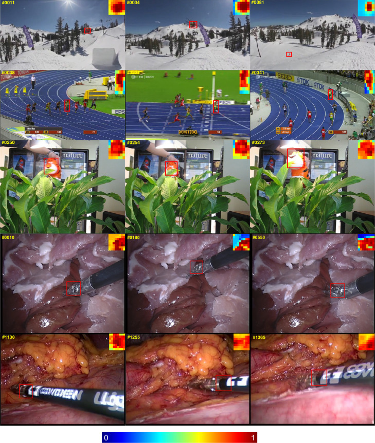
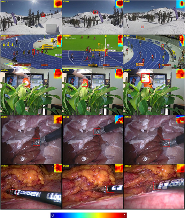
Unlike the weighting strategy in other patch-based methods (Chen, Yuan, Wu, Zhang, Zheng, 2013, Kim, Lee, Sim, Kim, 2015) by analysing the similarities between neighbouring patches, our patch weighting method is simple and straightforward to implement, the weight update for each patch is independent from each other, and only relies on the colour histogram based segmentation model. We show examples of the patch weight development in Fig. 3. The patch weight thumbnails are displayed on the top corner of each frame, which indicate the objectness in the bounding box and also reflect the object deformation over time. Since we update the segmentation model based on previous patch weights, and in turn the segmentation model facilitates updating the weight of all patches. This co-training strategy enhances the weight contrast between foreground and occluded patches, which suppresses background information efficiently.
Fig. 3.
Example patch weights are shown for the highlighted bounding box displayed in the top corner of the image. Warmer colour indicates higher foreground possibility.
3.3. Two-level sampling for scale estimation
The tracked object often undergoes complicated transformations during tracking, for example, deformation, scale variations, occlusion, etc. Fixed-scale bounding box estimation is ill-equipped to capture the accurate extents of the object, which would degrade the classifier performance by providing samples which are either partial cropped or include background information.
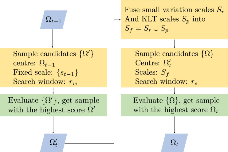
When locating the object in a new frame, all the bounding box candidates are collected within a search window, and the bounding box with the maximum classification score is selected to update the object location. Rather than making a suboptimal decision by choosing from fixed-scale samples, we augment training sample pool with multi-scale candidates, which is referred as two-level sampling strategy (see Fig. 4). On the first level, all the bounding box samples are extracted with fixed-scale (the object scale in frame ). The search window is centered at the with a height/width of rw, then the weighted patch-based descriptor of all candidates {Ω′} are fed into the classifier, and we select the bounding box with the maximum classification score not as the final decision, but as the search center for our second level. After first level, the rough location of the object is narrowed to a smaller area. We then set a smaller search window with search height/width of rs, centring at the bounding box selected in the first level, and we construct multi-scale candidates {Ω} within the search window. All the samples are evaluated by the classifier, and we select the bounding box Ωt of the sample with the maximum score as the final location of the object.
Fig. 4.
Two-level sampling strategy workflow.
Obviously, the scales of augmented samples are critical. We consider two complementary strategies that handle both incremental and abrupt scale variations. Firstly, to deal with relatively small scale changes between frames, we build a scale set Sr
| (8) |
where λ is a fixed value which is slightly larger than 1.0. It is set to accurately search the scale change. nr is the scale number in the scale set Sr. is the scale of the object in frame compared with the initial bounding box in the first frame. Considering object scale usually does not vary too much between frames, scale set Sr includes scales which are close to the previous frame.
Secondly, when object undergoes abrupt scale changes between frames, scale set Sr is unable to keep pace with the speed of the scale variations. To address this problem, we build an additional scale set Sp by incorporating Lucas–Kanade tracker (KLT) (Bouguet, 2001, Shi, Tomasi, 1994), which helps us estimate the scale change explicitly. We randomly pick npt points from each patch in the bounding box of frame and tracked all these points in the next frame t. With sufficient well-tracked points, we can estimate the scale variation between frames by comparing the distance changes of the tracked point pairs.
We illustrated the scale estimation by KLT tracker in Fig. 5. Let denotes one picked point in the previous frame and its matched point in the current frame t. We compute the distance between point-pair and the distance between the matched point-pair . For all the matched point pairs, we compute the distance ratio between the two frames
| (9) |
where V is the set with all the distance ratios. We sort V by value and pick the median element as the potential scale change of the object. To make scale estimation more robust, we uniformly sample the scales ranging between [1, sp] or [sp, 1] to construct the scale set Sp.
| (10) |
where np is the scale number in the scale set Sp. When the object is out-of-view, occluded or abruptly deforms, the ratio of well-tracked points will be low. In that case, the estimation from the KLT tracker will be unreliable. In our implementation, when the ratio is lower than 0.5, we then set therefore the scale set Sp will only add samples with the previous scale into the candidate pool. Only when there are enough points well tracked, the estimation from the KLT tracker will be trusted. We fuse these two complementary scale sets Sr and Sp into to enrich our sample candidate pool. To show the effectiveness, we evaluate our proposed tracker in Section 4 with or without scale set Sp estimated by the KLT tracker.
Fig. 5.
Illustration of scale estimation by using the KLT tracker. Random points located on the patches are picked in frame and are tracked in the next frame t by the KLT tracker, the distance ratio of point pairs (pi, pj) between two frames are used for scale estimation. We use 7 × 7 patch grids, resulting nφ=49 in the illustration.
3.4. Tracking framework
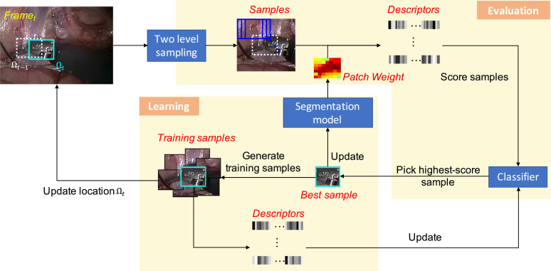
PAWSS can be combined with any tracking-by-detection method. We show the pipeline of the whole framework in Fig. 6. It includes two phases: evaluation and learning. The evaluation phase is to find the target in a new frame. Given the bounding box in the previous frame sample candidates are extracted in a search window, which centers at in the current frame t, unlike other tracking-by-detection approaches, we adapt a two-level sampling strategy for accurate scale estimation (Section 3.3). Via the colour-based segmentation model, weights of all patches are updated as in Section 3.2, and the descriptors of all samples are computed via patch weighting. Descriptors of all samples are fed into classifier and the one with the highest output score is picked as the best sample. The location Ωt of the best sample shows where the target is in the current frame at time t. Between frames, the target appearance changes due to deformation, occlusions, light and scale variations, therefore, the classifier and the segmentation model needs to be learnt online to keep up with the changes. The best sample among all samples represents the most similar one compared to the target. For one thing, pixel colour distribution of the best sample is used to update the segmentation model. For another, samples are extracted around the best sample in order to collect foreground and background information. Descriptors of all samples are computed and used to train the classifier online to better discriminate the target from neighbouring background. The procedure starts again for the next frame.
Fig. 6.
Tracking framework. Given the target location in the previous frame at time the framework is to predict the target location Ωt in the current frame at time t. The framework includes evaluation and learning phases. In evaluation phase, multi-scale samples are extracted via two-level sampling strategy, and then are fed into the classifier to pick the one with the highest score. The location of the sample is considered as the new location Ωt. The sample is also used for updating the segmentation model and the classifier in the learning phase.
In our implementation, we incorporate PAWSS into Struck Hare et al. (2011). The algorithm relies on an online structured output SVM learning framework which integrates learning and tracking. It directly predicts the location displacement between frame, avoiding the heuristic intermediate step for assigning binary labels to training samples, which achieves top performance in OTB dataset Wu et al. (2013).
4. Results
Implementation details: Our algorithm is publicly available online1 and is implemented in C++ and performs at about 7 frames per second with an i7-2.5 GHz CPU without any optimisation. We listed the parameter setting in Table 1. To illustrate the generalization of our proposed framework, we use the same parameter setting through all experiments. For structured output SVM, we are using a linear kernel and the parameters are empirically set as in Eqs. (3) and (5), in Eq. (8), the scale numbers of the scale set are . The number of extracted points from each patch . The updating threshold for the classifier is set as . For each sequence, we scale a frame to make sure the minimum side length of the bounding box is larger than 32 pixels, and the search window rw is fixed to where W and H represents the width and height of the scaled bounding box, respectively, and the search window rs is fixed to 5 pixels. We tested different low-level feature combinations in Section 4.1 and found that the combination of HSV colour and gradient features (HSV+G) achieves the best results. The patch number affects the tracking performance, too many patches increase the computation and too less patches do not robustly reflect the local appearance of the object. We tested different patch numbers, and selected to strike a performance balance.
Table 1.
Parameter setting of the framework in all experiments.
| Number of patches nφ | |
| Base of scale estimation λ | 1.003 |
| Number of scales for small scale changes nr | 11 |
| Number of scales for abrupt scale changes np | 11 |
| Updating factor of classifier η | 0.3 |
| Updating factor of segmentation model δ | 0.1 |
4.1. Online Tracking Benchmark (OTB)
OTB dataset (Wu et al., 2013) includes 50 sequences tagged with 11 attributes, which represent the challenging aspects for tracking such as illumination variation, occlusion, deformation et al. The tracking performance is quantitatively evaluated using both precision rate (PR) and success rate (SR), as defined in (Wu et al., 2013). PR/SR scores are depicted using precision plot and success plot, respectively. The precision plot shows the percentage of frames whose tracked centre is within certain Euclidean distance (20 pixels) from the centre of the ground truth. Success plot computes the percentage of frames whose intersection over union overlap with the ground truth annotation is within a threshold varying between 0 and 1, and the area under curve (AUC) is used for SR score. To evaluate the effectiveness of incorporating the scale set proposed by the KLT tracker, we provide two versions of our tracker as PAWSSa and PAWSSb: PAWSSa only includes scale set Sr, while PAWSSb includes both Sr and Sp for scale estimation.
Comparison using different features: Selecting right features to describe the object appearance plays a critical role in tracking. The most desirable feature property is its uniqueness so that the object can be distinguished from background. Raw intensities or colour features are usually used for histogram-based appearance representations, while edge or gradient information are less sensitive to illumination changes. Generally, many tracking approaches use a combination of these diverse features to represent the object (Hare, Saffari, Torr, 2011, Grabner, Grabner, Bischof, 2006, Li, Shen, Dick, Hengel, 2013). To evaluate the performance of our proposed approach, we tested different low-level features such as HSV colour, RGB colour, the combination of colour and gradient features (HSV+G, RGB+G) for constructing the descriptor in Table 5.1. The RGB histogram is 24-dimensional with 8 bins for each channel, and the HSV colour histogram is 20-dimensional including 8 bins for H and S channels respectively and 4 separate bins for V channel. The gradient histogram is 16-dimensional signed gradients ranging from 0 to 360∘. We also compared our tracker PAWSSa and PAWSSb with Struck (Hare et al., 2011) and SOWP (Kim et al., 2015). From Table 2, we observe: Augmenting colour with gradient histogram improves the tracking performance by providing diverse structural information of the object. In our experiments, the descriptor comprising combination of HSV colour and gradient features achieves the best results, we use this setting in the following evaluation.
Table 2.
The performance of the proposed algorithm compared with different low-level features. PAWSSa and PAWSSb tracker represents our tracker without and with the KLT tracker, respectively.
| PAWSSa | PAWSSb | |
|---|---|---|
| HSV | 0.731 / 0.528 | 0.742 / 0.545 |
| RGB | 0.764 / 0.552 | 0.749 / 0.544 |
| RGB+G | 0.838 / 0.605 | 0.840 / 0.607 |
| HSV+G | 0.889 / 0.635 | 0.897 / 0.649 |
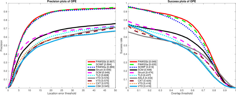
Comparison with state-of-the-art trackers: We use the evaluation toolkit provided by Wu et al. (2013) to generate the precision and success plots for the one pass evaluation (OPE) of the top 10 algorithms in Fig. 7. The toolkit includes 29 benchmark trackers, besides that we also include SOWP tracker. It is shown that PAWSSb achieves the best PR/SR scores among all the trackers. For a more detailed evaluation, we also compared our tracker with state-of-the-art trackers in Table 3. Notice that in all the attribute field, our tracker achieves either the best or the second best PR/SR scores. Our tracker achieves 36.7% gain in PR and 36.9% gain in SR over Struck (Hare et al., 2011). By using a simple patch weighting strategy and training with adaptive scale samples, the performance shows that our tracker provides comparable PR scores, and higher SR score compared with SOWP (Kim et al., 2015). PAWSSa tracker improves SR score by 2.6% considering gradually small changes between frames, PAWSSb improves SR score by 4.8% by incorporating scales estimated by the external KLT tracker. Specifically, when the object undergoes scare variation PAWSS achieves a performance gain of 10.3% in SR over SOWP.
Fig. 7.
Comparison of precision and success plots on OTB with the top 10 trackers; PR scores are illustrated with the threshold at 20 pixels and SR scores with the average overlap (AUC) in the legend.
Table 3.
Comparison of PR/SR score with state-of-the-art trackers including Struck (Hare et al., 2011), DSST (Danelljan et al., 2014), SAMF (Li and Zhu, 2014), FCNT (Wang et al., 2015) and SOWP (Kim et al., 2015) in the OPE based on the 11 sequence attributes: illumination variation (IV), scale variation (SV), occlusion (OCC), deformation (DEF), motion blur (MB), fast motion (FM), in-plane rotation (IPR), out-of-plane rotation (OPR), out-of-view (OV), background cluttered (BC) and low resolution (LR). The best and the second best results are shown in red and blue colours respectively.
 |
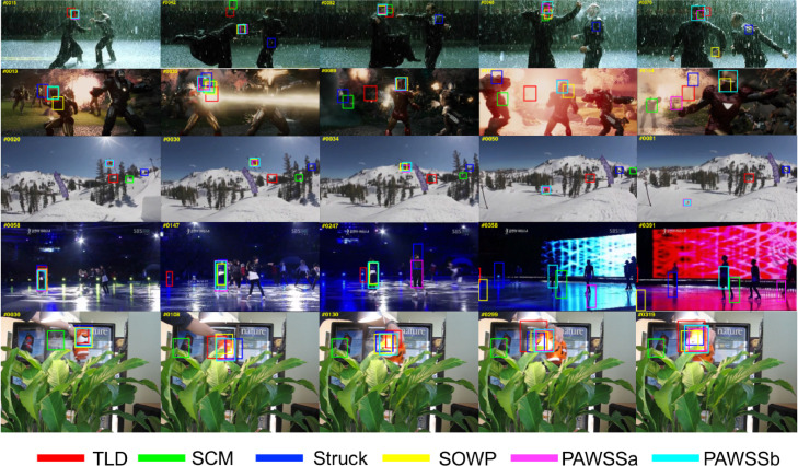
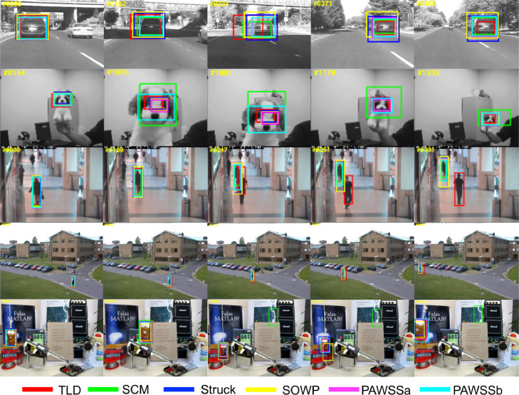
We show tracking results in Figs. 8 and 9 with the top trackers including TLD (Kalal et al., 2012), SCM (Zhong et al., 2012), Struck (Hare et al., 2011), SOWP (Kim et al., 2015) and the proposed PAWSSa and PAWSSb. In Fig. 8, five challenging sequences are selected from the benchmark dataset, which include illumination variation, scale variations, deformation, occlusion or background clusters. PAWSS can adapt when the object deforms in a complicated scene and track the target accurately. In Fig. 9, we select five representative sequences with different scale variations. PAWSS can well track the object with scale variation, while other trackers drift away. The results show that our proposed tracking framework PAWSS can track the object robustly through sequence by using the weighting strategy to suppress background information within the bounding box, and also by incorporating scale estimation allowing the classifier to train with adaptive scale samples. Please see the supplementary video for more sequence tracking results.
Fig. 8.
Comparison of the tracking results of our proposed tracker PAWSS with SOWP (Kim et al., 2015) and three conventional trackers: TLD (Kalal et al., 2012), SCM (Zhong et al., 2012) and Struck (Hare et al., 2011) on some especially challenging sequences in the benchmark.
Fig. 9.
Comparison of the tracking results of our proposed tracker PAWSS with SOWP (Kim et al., 2015) and three conventional trackers: TLD (Kalal et al., 2012), SCM (Zhong et al., 2012) and Struck (Hare et al., 2011) on some sequences with scale variations in the benchmark.
4.2. Visual Object Tracking (VOT) challenges
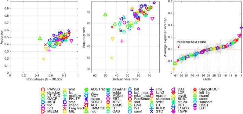
For completeness, we also validated our algorithm on VOT2014 (25 sequences) and VOT2015 (60 sequences) datasets. VOT datasets use ranking-based evaluation methodology: Accuracy and robustness. Similar to SR rate for OTB dataset, the accuracy measures overlap of the predicted result and the ground truth bounding box, while the robustness measures how many times the tracker fails during tracking. A failure is indicated whenever the tracker loses the target object which means the overlap becomes zero, and it will be re-initialized afterwards. All the trackers are evaluated, compared and ranked based on with respect to each measure separately using the official evaluation toolkit from the challenge.2
VOT2014 VOT2014 challenge includes two experiments: Baseline experiment and region-noise experiment. In baseline experiment, a tracker runs on all the sequences by initializing with the ground truth bounding box on the first frame; while in the region-noise experiment, the tracker is initialized with a random noisy bounding box with the perturbation in the 10% of the ground truth bounding box size. (Kristan et al., 2015b). The ranking plots with 38 trackers are shown in Fig. 10 for comparing PAWSS with the top three trackers: DSST (Danelljan et al., 2014), SAMF (Li and Zhu, 2014), KCF (Henriques et al., 2015) in Table 4. For both the experiments our PAWSS has lower accuracy score 0.58/0.55, but less failures 0.88/0.78 and have a second average rank. But considering the tracking process of the experiments: once a failure is detected, the tracker will be re-initialized, to eliminate the effect of achieving higher accuracy score by more re-initialization steps, we performed experiments without the re-initialization, also shown in Table 4. The results show that PAWSS has the highest accuracy score 0.51/0.48 among all the trackers without re-initialization, which means it is more robust than the other trackers.
Fig. 10.
The accuracy-robustness score and ranking plots with respect to the baseline and region-noise experiments of VOT2014 dataset. Tracker is better if its result is closer to the top-right corner of the plot.
Table 4.
The Accuracy (Acc.) and Robustness (Rob.) results of VOT2014 baseline and region-noise experiments with and without-re-initialization compared with the top trackers DSST (Danelljan et al., 2014), SAMF (Li and Zhu, 2014) and KCF (Henriques et al., 2015). The best and the second best results are shown in red and blue colours respectively.
VOT2015 Finally, we evaluated and compared PAWSS with 62 trackers on VOT2015 dataset. VOT2015 challenge only includes baseline experiment, and the ranking plots are shown in Fig. 11. In VOT2013 and VOT2014, average ranking measure is used to determine the performance of the trackers. Although average ranking has taken both accuracy and robustness measure into consideration, it is not theoretically representative as a concrete tracking performance. In VOT2015 (Kristan et al., 2015a), expected average overlap measure is introduced which combines both per-frame accuracies and failures in a principled manner. Compared with the average rank, expected overlap has a more clear practical interpretation.
Fig. 11.
The accuracy-robustness ranking plots and the expected overlap score ranking plot of VOT2015 dataset. Tracker is better if its result is closer to the top-right corner of the plot. The published sota bound is established based on top trackers in recent years. Any tracker with performance over the boundary is considered as a state-of-the-art tracker.
We list the score / rank and expected overlap of the top trackers from VOT2015 (Kristan et al., 2015a) which are either quite robust or accurate, the above VOT2014 top three trackers DSST (Danelljan et al., 2014), SAMF (Li and Zhu, 2014), KCF (Henriques et al., 2015),3 and the baseline NCC tracker in Table 5 and also shown in the expected average overlap plot Fig. 11. It can be shown that the average rank is not always consistent with the expected overlap. According to the paper (Kristan et al., 2015a), a VOT2015 published sota bound criteria (0.2) is established by averaging the tracker performance published in 2014/2015 from top computer vision conferences and journals. The tracker will be considered as a state-of-the-art tracker with performance over this boundary criteria. Our tracker PAWSS is well above the criteria, and is among those top trackers (ranks the 7-th, outperforming 54 trackers), also PAWSS achieves better than any of VOT2014 top trackers on VOT2015 dataset.
Table 5.
VOT2015 Accuracy (Acc.), Robustness (Rob.), Score/Ranking and expected overlap results from the top trackers of VOT2014, VOT2015 and the baseline tracker. The NCC tracker is VOT2015 baseline tracker. Trackers marked with † are submitted to VOT2015 without publication.
| Baseline |
Avg rank | Exp overlap | ||||
|---|---|---|---|---|---|---|
| Acc. |
Rob. |
|||||
| Score | Rank | Failure | Rank | |||
| MDNet Nam and Han (2015) | 0.59 | 2.03 | 0.77 | 5.68 | 3.86 | 0.378 |
| DeepSRDCF Danelljan et al. (2015a) | 0.56 | 5.92 | 1.00 | 8.38 | 7.15 | 0.318 |
| EBT Wang and Yeung (2014) | 0.45 | 15.48 | 0.81 | 7.23 | 11.36 | 0.313 |
| SRDCT Danelljan et al. (2015b) | 0.55 | 5.25 | 1.18 | 9.83 | 7.54 | 0.288 |
| LDP Lukežič et al. (2016) | 0.49 | 12.08 | 1.30 | 13.07 | 12.58 | 0.279 |
| sPST Hua et al. (2015) | 0.54 | 6.57 | 1.42 | 12.57 | 9.57 | 0.277 |
| PAWSSb | 0.53 | 7.75 | 1.28 | 11.22 | 9.49 | 0.266 |
| NSAMF† | 0.53 | 7.02 | 1.45 | 10.1 | 8.56 | 0.254 |
| RAJSSC Zhang et al. (2015) | 0.57 | 4.23 | 1.75 | 13.87 | 9.05 | 0.242 |
| RobStruck† | 0.49 | 11.45 | 1.58 | 14.82 | 13.14 | 0.220 |
| DSST Danelljan et al. (2014) | 0.53 | 8.05 | 2.72 | 26.02 | 17.04 | 0.172 |
| SAMF Li and Zhu (2014) | 0.51 | 7.98 | 2.08 | 18.08 | 13.03 | 0.202 |
| KCF Henriques et al. (2015) | 0.47 | 12.83 | 2.43 | 21.85 | 17.34 | 0.171 |
| NCC* | 0.48 | 12.47 | 8.18 | 50.33 | 31.4 | 0.080 |
4.3. Surgical instrument tracking
PAWSS is a general tracking framework, we also want to evaluate its performance on both ex vivo and in vivo surgical instrument sequences. In the Endoscopic vision MICCAI2015 Challenge.,4 one of the sub-challenge focuses on comparing different vision-based methods for tracking conventional and articulated laparoscopic instruments in robotic surgery. The dataset has not released ground truth for test data. The official evaluation categorized conventional laparoscopic instrument test set according to the challenging factors including bleeding (Cblood), smoke (Csmoke), instrument occlusions (Cocclusion), multiple instruments (Cmultiple) and surgical objects such as meshes and clips (Cobjects). And the robotic laparoscopic instrument dataset includes sequences with multiple instruments (Cmultiple). For evaluating the tracking performance, Euclidean distance of the centre point between the ground truth and the tracking result of training data is computed and compared separately for these challenging factors. We submitted our proposed method to the challenge, and obtained the performance comparison from the official report.
EndoVis Articulated Robotic Laparoscopic instrument dataset The articulated instrument dataset is from ex vivo interventions, and the sequences are collected using the da Vinci® (Intuitive Surgical Inc., CA) system with porcine tissue samples. Example frames from each sequence are shown in Fig. 12 (a). The dataset is divided into training and test data. Training data contains four 45 seconds surgery video sequences. For each instrument, the tracked point of the instrument is defined as the intersection between the instrument axis and the border between the shaft and the manipulator. The annotation includes pixel coordinates of the tracked point (Fig. 12 (b)). Test data is composed of 15 additional seconds video from each of the training sequence, and two additional new 60 s video sequences.
Fig. 12.
(a) Example frame from each sequence of EndoVis articulated surgical instrument dataset; (b) The original annotation includes the position of the tracked point, in our annotation, we relabeled the tracked point and also added new annotations for the Head and Shaft points.
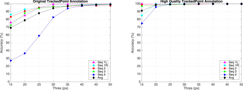
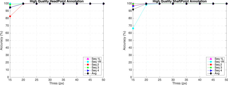
Original annotation We have summarized the frame number for each sequence and have shown the accuracy evaluation separately in the original annotation section of Table 6 and Fig. 14 Left. The accuracy is defined as the percentage of tracked frames within the error threshold. Distance (pixels) is averaged over correctly tracked frames. In Fig. 14, it shows accuracy under different threshold. In four train sequences, there are five instruments to be tracked. The average accuracy score for train data is 79.01% for 20 pixel threshold, with a distance error of 8.00 pixels. It is noted that the accuracy score (36.55% for 20 pixel threshold) for sequence 4 is relatively lower compared with the rest sequences. As we have summarized, the target is out of view several times in sequence 4, reaching 67 frames out of 1123 frames. Tracking-by-detection methods typically cannot handle out-of-view scenario without additional re-detection module. The underlying assumption is that the target is always in frame view, which means Whenever the target is out of frame, the tracker will gradually drift away. This explains the low accuracy of the performance, if the threshold is increased to 30 pixels, the performance has significantly improved, achieving 82.67% for accuracy.
Table 6.
Accuracy of EndoVis articulated robotic surgical instrument training data for the tracked point.
| Seq 1L | Seq 1R | Seq 2 | Seq 3 | Seq 4 | Whole | |
|---|---|---|---|---|---|---|
| Original annotation | ||||||
| In-view (IV) and Out-of-view (OV) Frame Number | ||||||
| IV | 1107 | 1107 | 1096 | 1118 | 1056 | 5484 |
| OV | 0 | 0 | 29 | 6 | 67 | 102 |
| Total | 1107 | 1107 | 1125 | 1124 | 1123 | 5586 |
| Accuracy ( px) | ||||||
| Acc. (%) | 85.00 | 92.86 | 90.60 | 88.10 | 36.55 | 79.01 |
| Dist. (px) | 7.42 | 7.07 | 7.41 | 9.64 | 9.26 | 8.00 |
| Accuracy ( px) | ||||||
| Acc. (%) | 99.37 | 96.93 | 96.35 | 95.80 | 82.67 | 94.33 |
| Dist. (px) | 9.76 | 7.80 | 8.36 | 10.71 | 18.07 | 10.67 |
| High quality annotation | ||||||
| In-view (IV) and Out-of-view (OV) frame number | ||||||
| IV | 1107 | 1107 | 1099 | 1105 | 1066 | 5484 |
| OV | 0 | 0 | 26 | 19 | 57 | 102 |
| Total | 1107 | 1107 | 1125 | 1124 | 1123 | 5586 |
| Accuracy ( px) | ||||||
| Acc. (%) | 100.0 | 99.73 | 98.91 | 98.28 | 95.78 | 98.56 |
| Dist. (px) | 4.89 | 9.87 | 3.29 | 4.31 | 11.13 | 6.65 |
| Accuracy ( px) | ||||||
| Acc. (%) | 100.0 | 100.0 | 99.36 | 99.46 | 99.72 | 99.71 |
| Dist. (px) | 4.89 | 9.90 | 3.38 | 4.56 | 11.57 | 6.83 |
Fig. 14.
Tracking accuracy of EndoVis Articulated Robotic Surgical Instrument training data under different accuracy threshold with the original and high-quality annotations.
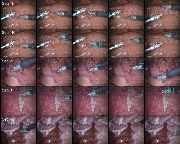
We show some tracking result examples in Fig. 13. The tracked point and bounding box are shown in cyan colour, with the ground truth point shown in green colour. The first column is the first frame of each sequence. As we can see, the quality of the annotation is not consistent through the whole sequence. On certain frames, the annotation is drifted and is not labelled where it is supposed to be. This would certainly affect our performance evaluation result. It is also observed that whenever the instrument is close to the frame border, the tracker will stick to the border and not track the instrument well.
Fig. 13.
Result example frames from each sequence of the EndoVis articulated robotic surgical instrument dataset. The result bounding box and centre point is represented in cyan colour, and the ground truth centre point is represented in green colour. (For interpretation of the references to colour in this figure legend, the reader is referred to the web version of this article.)
High quality annotation The original annotation is retrieved from the robotic system, which includes the location of the intersection point between the instrument axis and the border between plastic and metal on the shaft, normalized Shaft-to-Head axis vector and the clasper angle. Since the original annotation does not provide consistent ground truth, the accuracy result does not reflect true performance. We manually labelled the training data, and construct a high quality annotation. In this annotation, we labelled multiple joints of the instrument including the original tracked point, the Head and Shaft point. The original and our proposed annotations are demonstrated in Fig. 12 (b).
We also tracked and evaluated on the Head and Shaft points we defined in our high quality annotation in the high quality annotation section of Table 6 and Fig. 14 right. With new annotation, our average accuracy has increased to 98.56% for 20 pixel threshold, with distance error of 6.65 pixels.
The tracking accuracy evaluation results are displayed in Table 7 and Fig. 15. Our average accuracy has reached 99.96% and 99.68% for 20 pixels threshold, with distance error of 5.68 and 6.51 pixels, respectively.
Table 7.
Accuracy of EndoVis articulated robotic surgical instrument train data for Head and Shaft points with high quality annotation.
| Seq 1L | Seq 1R | Seq 2 | Seq 3 | Seq 4 | Whole | |
|---|---|---|---|---|---|---|
| In-view (IV) and Out-of-view (OV) frame number | ||||||
| IV | 1107 | 1107 | 1125 | 1124 | 1123 | 5586 |
| OV | 0 | 0 | 0 | 0 | 0 | 0 |
| Total | 1107 | 1107 | 1125 | 1124 | 1123 | 5586 |
| Head accuracy ( px) | ||||||
| Acc. (%) | 100.0 | 100.0 | 99.82 | 100.0 | 100.0 | 99.96 |
| Dist. (px) | 3.06 | 4.10 | 10.32 | 4.52 | 6.33 | 5.68 |
| Shaft accuracy ( px) | ||||||
| Acc. (%) | 100.0 | 98.46 | 100 | 99.91 | 100 | 99.68 |
| Dist. (px) | 2.48 | 12.08 | 6.82 | 4.79 | 6.48 | 6.51 |
Fig. 15.
Accuracy of EndoVis Articulated Robotic Surgical Instrument training data under different accuracy threshold with high quality annotation.
Comparison performance In Table 8, the distance error (pixel) was computed and compared separately for challenging factor multiple instrument (Cmultiple) with all the submitted methods KIT, UGA, MOD and our method PAWSS. From official report, PAWSS outperforms all the other methods with the lowest average distance error 29.66 pixels.
Table 8.
Distance (pixel) comparison with all the submitted methods for the tracked Point of the robotic laparoscopic instrument test set. Multiple instrument challenging subset is evaluated separately.
| Cmultiple | Whole | |
|---|---|---|
| KIT | 113.91 | 106.60 |
| UGA | 40.73 | 34.94 |
| MOD | 45.12 | 40.16 |
| PAWSS | 38.36 | 29.66 |
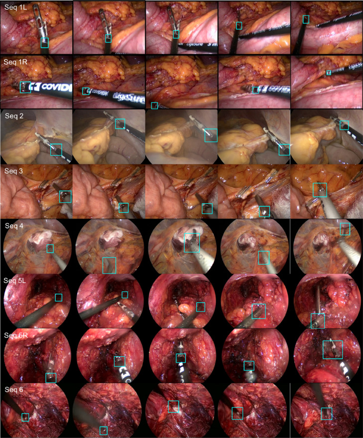
EndoVis Conventional Laparoscopic Instrument Dataset The conventional instrument dataset contains six in vivo sequences, which are collected from complete laparoscopic colorectal interventions. Similar to the robotic instrument dataset, training data contains 45 s video sequences, and test data is made up of 15 additional seconds videos for each sequence and two new 60 s videos. Compared to ex vivo robotic instrument dataset, these sequences reflect complex challenges during surgery, including smoke, bleeding, blurry and various kinds of instruments. In Table 9, the distance error (pixel) was computed and compared separately for each challenging factor with all the submitted methods KIT, UGA and our method PAWSS. From the official report, PAWSS outperforms all the other methods in every challenging subset with the lowest average distance error 96.78 pixels. We show some tracking result examples in Fig. 17. The tracked point is shown in cyan colour, and the first column is the first frame of each sequence in test set. (Fig. 16)
Table 9.
Distance (pixel) comparison with all the submitted methods for the tracked point of the conventional laparoscopic instrument test set. Various challenging subsets are evaluated separately.
| Cblood | Cmultiple | Cobjects | Cocclusion | Csmoke | Whole | |
|---|---|---|---|---|---|---|
| KIT | 233.62 | 220.87 | 117.23 | 225.58 | 193.85 | 178.89 |
| UGA | 276.44 | 235.42 | 228.04 | 193.82 | 231.87 | 217.91 |
| PAWSS | 181.59 | 110.85 | 68.29 | 87.11 | 96.31 | 96.78 |
Fig. 17.
Result example frames from each test sequence of the EndoVis conventional surgical instrument dataset. The result bounding box is represented in cyan colour.
Fig. 16.
(a) Example frame from each sequence of EndoVis articulated surgical instrument training dataset; (b) The annotation includes the position of the tracked point.
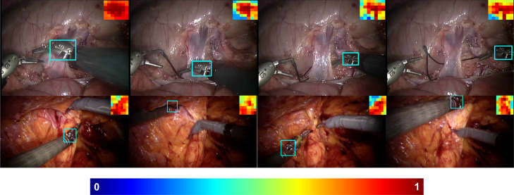
In vivo surgical instrument experiments We also test on some other in vivo sequences and show the result in Fig. 18. As we can see, the tracker works well even under complex in vivo environment. The video is submitted to display the tracking results for the whole sequences.
Fig. 18.
Instrument Tracking result with patch weight displayed in the top corner of the image.
5. Conclusions
In this paper, we propose a tracking-by-detection framework, called PAWSS, for online object tracking. It uses a colour-based segmentation model to suppress background information by assigning weights to the patch-wise descriptor. We incorporate scale estimation into the framework, allowing the tracker to handle both incremental and abrupt scale variations between frames. The learning component in our framework is based on Struck, but we would like to point out that theoretically our proposed method can also support other online learning techniques with effective background suppression and scale adaption.
The performance of our tracker is thoroughly evaluated on OTB, VOT2014 and VOT2015 datasets and compared with recent state-of-the-art trackers. Results demonstrate that PAWSS achieves the best performance in both PR and SR in OPE for OTB dataset. It outperforms Struck by 36.7% and 36.9% in PR/SR scores. Also, it provides a comparable PR score, and improves SR score by 4.8% over SOWP. On VOT2014 dataset, PAWSS has relatively lower accuracies but the lowest failure rate among the top trackers, we evaluated without re-initialization, and achieves the highest performance. Also on VOT2015 dataset, PAWSS is considered state-of-the-art and is among the top trackers.
For instrument tracking, we also qualitatively and quantitatively evaluated our tracker on public EndoVis robotic and conventional surgical instrument datasets, and in vivo surgical instrument sequences. We compared our result with the official GT for the Tracked Point on the robotic instrument dataset, and tracking accuracy reached 79.01% with 20 pixel threshold. As we have shown, the official annotation is not quality consistent, we manually created a high quality multi joint annotation for the dataset. We tested multiple joints (Tracked Point, Head and Shaft Point) on the dataset, and our performance accuracy increased over 98% for all the joints with 20 pixel threshold. From the official challenge report, Our method has shown the lowest tracking error for both robotic and conventional instrument datasets, and it also shown its excellent tracking ability with in vivo sequences dealing with complicated surgical environment. Our framework is designed for general single object tracking. It does not require prior information about the target or any offline training to achieve robust and real-time performance. We would also like to discuss the limitations of our framework. First, if the target disappears and reappears from the scene, the framework does not recover. Second, the target position is represented by rectangle bounding box. Even with the assistance of the segmentation model to distinguish foreground and background, the assumption is that the target occupies most area of the bounding box. If the target only occupies small fraction, the classifier would be polluted and misled by background information and can easily cause tracking failure. In the future, we would like to focus on re-detection module and semantic foreground segmentation.
Declarations of interest
None
Acknowledgements
Xiaofei Du is supported by the China Scholarship Council (CSC) scholarship. The work has been carried out as part of an internship at Wirewax Ltd, London, UK. The work was supported by the EPSRC (EP/N013220/1, EP/N022750/1, EP/N027078/1, NS/A000027/1, EP/P012841/1), The Wellcome Trust (WT101957, 201080/Z/16/Z) and the EU-Horizon 2020 project EndoVESPA (H2020-ICT-2015-688592). This work was supported by the Wellcome/EPSRC Centre for Interventional and Surgical Sciences (WEISS) at UCL (203145Z/16/Z) and EPSRC (EP/N027078/1, EP/P012841/1, EP/P027938/1, EP/R004080/1).
Biographies
Xiaofei Du received a bachelor degree in Telecommunications at Nanjing University of Posts and Telecommunications and a master in Biomedical Engineering from Tsinghua University, China. Currently, she is a Ph.D student at Centre for Medical Image Computing (CMIC) of University College London (UCL). Her research interests include surgical vision and medical image computing.
Maximilian Allan is a computer vision engineer at Intuitive Surgical in Sunnyvale, CA. He completed his PhD in surgical robot vision with Dan Stoyanov at University College London (UCL) in 2017 working on instrument detection and tracking for the da Vinci robot. He obtained a Master degree in computer science from Imperial College London in 2011 and a Bachelors in physics from Kings College London in 2010.
Sebastian Bodenstedt got a Ph.D degree in Karlsruhe Institute of Technology (KIT), he is currently a postdoc in National Center for Tumor Diseases Dresden, Germany. His research interests include medical robots and computer assisted interventions.
Lena Maier-Hein received the Ph.D degree from Karlsruhe Institute of Technology (KIT) with distinction and conducted her postdoctoral research in the Division of Medical and Biological Informatics at the German Cancer Research Center (DKFZ) and at the Hamlyn Centre for Robotics Surgery at Imperial College London. As an independent junior group leader at the DKFZ, she is now working in the field of computer-assisted medical interventions with a focus on multi-modal image processing, knowledge-based systems and computational biophotonics.
Stefanie Speidel is a Professor in National Center for Tumor Diseases Dresden, Germany. Her research interests include multimodal analysis of intraoperative data, biomechanical soft-tissue navigation as well as surgical data science.
Alessio Dore got a Ph.D degree in the Department of Biophysical and Electronic Engineering (DIBE), University of Genova, Italy. He is a senior data scientist and a manager at Deliveroo, London, UK.
Danail Stoyanov received a BEng degree from King’s College London and a Ph.D degree in medical image computing from Imperial College London. He was a Royal Academy of Engineering Research Fellow when he joined the Centre for Medical Image Computing and the Department of Computer Science, University College London (UCL). He is now a Professor at UCL and an EPSRC Early Career Research Fellow. He is also Chief Scientist at Digital Surgery, London, UK. His research interests include computer assisted interventions, medical image computing and medical robotics.
Footnotes
This is an improved version of the original tracker.
Supplementary material associated with this article can be found, in the online version, at doi:https://doi.org/10.1016/j.media.2019.07.002 .
Contributor Information
Xiaofei Du, Email: xiaofei.du.13@ucl.ac.uk.
Maximilian Allan, Email: Max.allan@intusurg.com.
Sebastian Bodenstedt, Email: sebastian.bodenstedt@nct-dresden.de.
Lena Maier-Hein, Email: l.maier-hein@dkfz-heidelberg.de.
Stefanie Speidel, Email: stefanie.speidel@nct-dresden.de.
Alessio Dore, Email: alessio.dore@deliveroo.co.uk.
Danail Stoyanov, Email: danail.stoyanov@ucl.ac.uk.
Appendix A. Supplementary materials
Supplementary Raw Research Data. This is open data under the CC BY license http://creativecommons.org/licenses/by/4.0/
Supplementary Raw Research Data. This is open data under the CC BY license http://creativecommons.org/licenses/by/4.0/
References
- Allan M., Chang P.-L., Ourselin S., Hawkes D.J., Sridhar A., Kelly J., Stoyanov D. Medical Image Computing and Computer-Assisted Intervention (MICCAI), 2015 International Conference on. Springer; 2015. Image based surgical instrument pose estimation with multi-class labelling and optical flow; pp. 331–338. [Google Scholar]
- Allan M., Ourselin S., Hawkes D.J., Kelly J.D., Stoyanov D. 3-D pose estimation of articulated instruments in robotic minimally invasive surgery. IEEE Trans. Med. Imaging. 2018;37(5):1204–1213. doi: 10.1109/TMI.2018.2794439. [DOI] [PubMed] [Google Scholar]
- Allan M., Ourselin S., Thompson S., Hawkes D.J., Kelly J., Stoyanov D. Toward detection and localization of instruments in minimally invasive surgery. Biomed. Eng. IEEE Trans. 2013;60(4):1050–1058. doi: 10.1109/TBME.2012.2229278. [DOI] [PubMed] [Google Scholar]
- Allan M., Thompson S., Clarkson M.J., Ourselin S., Hawkes D.J., Kelly J., Stoyanov D. Information Processing in Computer-assisted Interventions, International Conference on. Springer; 2014. 2d-3d pose tracking of rigid instruments in minimally invasive surgery; pp. 1–10. [Google Scholar]
- Avidan S. Ensemble tracking. Pattern Anal. Mach. Intell. IEEE Trans. 2007;29(2):261–271. doi: 10.1109/TPAMI.2007.35. [DOI] [PubMed] [Google Scholar]
- Bouguet J.-Y. Pyramidal implementation of the affine Lucas Kanade feature tracker description of the algorithm. Intel Corp. 2001;5(1–10):4. [Google Scholar]
- Cano A.M., Gayá F., Lamata P., Sánchez-González P., Gómez E.J. International Symposium on Biomedical Simulation. Springer; 2008. Laparoscopic tool tracking method for augmented reality surgical applications; pp. 191–196. [Google Scholar]
- Chen D., Yuan Z., Wu Y., Zhang G., Zheng N. Proceedings of the IEEE International Conference on Computer Vision. 2013. Constructing adaptive complex cells for robust visual tracking; pp. 1113–1120. [Google Scholar]
- Collins R.T., Liu Y., Leordeanu M. Online selection of discriminative tracking features. Pattern Anal. Mach. Intell. IEEE Trans. 2005;27(10):1631–1643. doi: 10.1109/TPAMI.2005.205. [DOI] [PubMed] [Google Scholar]
- Comaniciu D., Ramesh V., Meer P. Kernel-based object tracking. Pattern Anal. Mach. Intell. IEEE Trans. 2003;25(5):564–577. [Google Scholar]
- Danelljan M., Häger G., Khan F., Felsberg M. British Machine Vision Conference, Nottingham, September 1–5, 2014. BMVA Press; 2014. Accurate scale estimation for robust visual tracking. [Google Scholar]
- Danelljan M., Hager G., Shahbaz Khan F., Felsberg M. Proceedings of the IEEE International Conference on Computer Vision Workshops. 2015. Convolutional features for correlation filter based visual tracking; pp. 58–66. [Google Scholar]
- Danelljan M., Hager G., Shahbaz Khan F., Felsberg M. Proceedings of the IEEE International Conference on Computer Vision. 2015. Learning spatially regularized correlation filters for visual tracking; pp. 4310–4318. [Google Scholar]
- Duffner S., Garcia C. Computer Vision (ICCV), 2013 IEEE International Conference on. IEEE; 2013. Pixeltrack: a fast adaptive algorithm for tracking non-rigid objects; pp. 2480–2487. [Google Scholar]
- Gao J., Ling H., Hu W., Xing J. Computer Vision–ECCV 2014. Springer; 2014. Transfer learning based visual tracking with gaussian processes regression; pp. 188–203. [Google Scholar]
- Godec M., Roth P.M., Bischof H. Hough-based tracking of non-rigid objects. Comput. Vision Image Underst. 2013;117(10):1245–1256. [Google Scholar]
- Grabner H., Grabner M., Bischof H. BMVC. Vol. 1. 2006. Real-time tracking via on-line boosting; p. 6. [Google Scholar]
- Hare S., Saffari A., Torr P.H. Computer Vision (ICCV), 2011 IEEE International Conference on. IEEE; 2011. Struck: structured output tracking with kernels; pp. 263–270. [Google Scholar]
- He S., Yang Q., Lau R., Wang J., Yang M.-H. Proceedings of the IEEE Conference on Computer Vision and Pattern Recognition. 2013. Visual tracking via locality sensitive histograms; pp. 2427–2434. [Google Scholar]
- Henriques J.F., Caseiro R., Martins P., Batista J. High-speed tracking with kernelized correlation filters. IEEE Trans. Pattern Anal. Mach.Intell. 2015;37(3):583–596. doi: 10.1109/TPAMI.2014.2345390. [DOI] [PubMed] [Google Scholar]
- Hua Y., Alahari K., Schmid C. Proceedings of the IEEE International Conference on Computer Vision. 2015. Online object tracking with proposal selection; pp. 3092–3100. [Google Scholar]
- Kalal Z., Mikolajczyk K., Matas J. Tracking-learning-detection. Pattern Anal. Mach. Intell. IEEE Trans. 2012;34(7):1409–1422. doi: 10.1109/TPAMI.2011.239. [DOI] [PubMed] [Google Scholar]
- Kim H.-U., Lee D.-Y., Sim J.-Y., Kim C.-S. Proceedings of the IEEE International Conference on Computer Vision. 2015. Sowp: spatially ordered and weighted patch descriptor for visual tracking; pp. 3011–3019. [Google Scholar]
- Kristan M., Matas J., Leonardis A., Felsberg M., Cehovin L., Fernández G., Vojir T., Hager G., Nebehay G. Proceedings of the IEEE international conference on computer vision workshops. 2015. The visual object tracking vot2015 challenge results; pp. 1–23. [Google Scholar]
- Kristan M., Pflugfelder R., Leonardis A., Matas J., Čehovin L., Nebehay G., Vojíř T., Fernández G., Lukežič A. Computer Vision - ECCV 2014 Workshops: Zurich, Switzerland, September 6–7 and 12, 2014, Proceedings, Part II. 2015. The visual object tracking vot2014 challenge results; pp. 191–217. [Google Scholar]
- Lee D.-Y., Sim J.-Y., Kim C.-S. Proceedings of the IEEE Conference on Computer Vision and Pattern Recognition. 2014. Visual tracking using pertinent patch selection and masking; pp. 3486–3493. [Google Scholar]
- Li X., Shen C., Dick A., Hengel A. Proceedings of the IEEE Conference on Computer Vision and Pattern Recognition. 2013. Learning compact binary codes for visual tracking; pp. 2419–2426. [Google Scholar]
- Li Y., Zhu J. Computer Vision-ECCV 2014 Workshops. Springer; 2014. A scale adaptive kernel correlation filter tracker with feature integration; pp. 254–265. [Google Scholar]
- Lukežič A., Čehovin L., Kristan M. Deformable parts correlation filters for robust visual tracking. arXiv preprint arXiv:1605.03720. 2016 doi: 10.1109/TCYB.2017.2716101. [DOI] [PubMed] [Google Scholar]
- Nam H., Han B. Learning multi-domain convolutional neural networks for visual tracking. arXiv preprint arXiv:1510.07945. 2015 [Google Scholar]
- Pezzementi Z., Voros S., Hager G.D. Robotics and Automation (ICRA), 2009 IEEE International Conference on. IEEE; 2009. Articulated object tracking by rendering consistent appearance parts; pp. 3940–3947. [Google Scholar]
- Reiter A., Allen P.K. Intelligent Robots and Systems (IROS), 2010 IEEE/RSJ International Conference on. IEEE; 2010. An online learning approach to in-vivo tracking using synergistic features; pp. 3441–3446. [Google Scholar]
- Shi J., Tomasi C. Computer Vision and Pattern Recognition, 1994. Proceedings CVPR ’94., 1994 IEEE Computer Society Conference on. 1994. Good features to track; pp. 593–600. [Google Scholar]
- Tonet O., Thoranaghatte R.U., Megali G., Dario P. Tracking endoscopic instruments without a localizer: a shape-analysis-based approach. Comput. Aided Surg. 2007;12(1):35–42. doi: 10.3109/10929080701210782. [DOI] [PubMed] [Google Scholar]
- Tsochantaridis I., Joachims T., Hofmann T., Altun Y. Journal of Machine Learning Research. 2005. Large margin methods for structured and interdependent output variables; pp. 1453–1484. [Google Scholar]
- Uecker D.R., Wang Y., Lee C., Wang Y. Automated instrument tracking in robotically assisted laparoscopic surgery. J. Image Guided Surg. 1995;1(6):308–325. doi: 10.1002/(SICI)1522-712X(1995)1:6<308::AID-IGS3>3.0.CO;2-E. [DOI] [PubMed] [Google Scholar]
- Wang L., Ouyang W., Wang X., Lu H. Proceedings of the IEEE International Conference on Computer Vision. 2015. Visual tracking with fully convolutional networks; pp. 3119–3127. [Google Scholar]
- Wang N., Yeung D.-Y. ICML. 2014. Ensemble-based tracking: aggregating crowdsourced structured time series data; pp. 1107–1115. [Google Scholar]
- Wei G.-Q., Arbter K., Hirzinger G. Real-time visual servoing for laparoscopic surgery. controlling robot motion with color image segmentation. IEEE Eng. Med. Biol. Mag. 1997;16(1):40–45. doi: 10.1109/51.566151. [DOI] [PubMed] [Google Scholar]
- Wu Y., Lim J., Yang M.-H. Computer vision and pattern recognition (CVPR), 2013 IEEE Conference on. IEEE; 2013. Online object tracking: a benchmark; pp. 2411–2418. [Google Scholar]
- Ye M., Zhang L., Giannarou S., Yang G.-Z. edical Image Computing and Computer-Assisted Intervention (MICCAI), 2016 International Conference on, Springer; 2016. Real-time 3d tracking of articulated tools for robotic surgery; pp. 386–394. [Google Scholar]
- Zhang L., van der Maaten L.J. Preserving structure in model-free tracking. Pattern Anal. Mach. Intell. IEEE Trans. 2014;36(4):756–769. doi: 10.1109/TPAMI.2013.221. [DOI] [PubMed] [Google Scholar]
- Zhang L., Ye M., Chan P.-L., Yang G.-Z. Real-time surgical tool tracking and pose estimation using a hybrid cylindrical marker. Int. J. Comput. Assist.Radiol. Surg. 2017;12(6):921–930. doi: 10.1007/s11548-017-1558-9. [DOI] [PMC free article] [PubMed] [Google Scholar]
- Zhang M., Xing J., Gao J., Shi X., Wang Q., Hu W. Proceedings of the IEEE International Conference on Computer Vision Workshops. 2015. Joint scale-spatial correlation tracking with adaptive rotation estimation; pp. 32–40. [Google Scholar]
- Zhang X., Payandeh S. Application of visual tracking for robot-assisted laparoscopic surgery. J. Field Robot. 2002;19(7):315–328. [Google Scholar]
- Zhong W., Lu H., Yang M.-H. Computer vision and pattern recognition (CVPR), 2012 IEEE Conference on. IEEE; 2012. Robust object tracking via sparsity-based collaborative model; pp. 1838–1845. [Google Scholar]
Associated Data
This section collects any data citations, data availability statements, or supplementary materials included in this article.
Supplementary Materials
Supplementary Raw Research Data. This is open data under the CC BY license http://creativecommons.org/licenses/by/4.0/
Supplementary Raw Research Data. This is open data under the CC BY license http://creativecommons.org/licenses/by/4.0/


