Transient Deformation in California From Two Decades of GPS Displacements: Implications for a Three‐Dimensional Kinematic Reference Frame

Abstract

Our understanding of plate boundary deformation has been enhanced by transient signals observed against the backdrop of time‐independent secular motions. We make use of a new analysis of displacement time series from about 1,000 continuous Global Positioning System (GPS) stations in California from 1999 to 2018 to distinguish tectonic and nontectonic transients from secular motion. A primary objective is to define a high‐resolution three‐dimensional reference frame (datum) for California that can be rapidly maintained with geodetic data to accommodate both secular and time‐dependent motions. To this end, we compare the displacements to those predicted by a horizontal secular fault slip model for the region and construct displacement and strain rate fields. Over the past 19 years, California has experienced 19 geodetically detectable earthquakes and widespread postseismic deformation. We observe postseismic strain rate variations as large as 1,000 nstrain/year with moment releases equivalent up to an Mw6.8 earthquake. We find significant secular differences up to 10 mm/year with the fault slip model, from the Mendocino Triple Junction to the southern Cascadia subduction zone, the northern Basin and Range, and the Santa Barbara channel. Secular vertical uplift is observed across the Transverse Ranges, Coastal Ranges, Sierra Nevada, as well as large‐scale postseismic uplift after the 1999 Mw7.1 Hector Mine and 2010 Mw7.2 El Mayor‐Cucapah earthquakes. We also identify areas of vertical land motions due to anthropogenic, natural, and magmatic processes. Finally, we demonstrate the utility of the kinematic datum by improving the accuracy of high‐spatial‐resolution 12‐day repeat‐cycle Sentinel‐1 Interferometric Synthetic Aperture Radar displacement and velocity maps.

Key Points

• Displacement fields from 19 years of GPS data in California are preferable to velocity fields in characterizing 3‐D transient motions

• Mapping of secular and transient motions at high temporal and spatial resolution is required for maintaining a 3‐D kinematic reference frame

• Displacement fields derived from continuous GPS and InSAR provide 200‐m resolution with millimeter‐level velocity uncertainties

1. Introduction

Over the last three decades, space geodesy has been widely used to observe and model crustal deformation at local to global scales to better understand the underlying physical processes of tectonic plate motion, plate boundary deformation, earthquakes, tsunamis, and volcanos (Bock & Melgar, 2016; Burgmann & Thatcher, 2013). Understanding these processes is critical to society's efforts to mitigate the detrimental effects of natural hazards on civilian life and property. The presence of transient deformation (e.g., postseismic, fault creep, and slow slip events) atop time‐independent secular motions is improving our understanding of physical processes and necessitating a reassessment of seismic risk. It is therefore critical to be able to identify and characterize transients and distinguish them from secular motions.

Our focus is on transient deformation in California, a region of intense study; its morphological features and major fault zones are well known (Figure 1; Field et al., 2014; Plesch et al., 2007). For example, the San Andreas Fault (SAF) system is a major plate boundary having both secular motions and transients. California has a long seismic history with devastating earthquakes. The 1906 Mw7.9–8.0 Great San Francisco earthquake killed more than 600 people and caused about $400 million (in 1906 dollars) in damage. The 1994 Mw6.7 Northridge earthquake in Los Angeles killed 57 people, injured more than 8,700, and incurred damages valued at up to tens of billions of dollars. Ongoing tectonic and nontectonic deformations punctuated by medium to large earthquakes and time‐dependent motions also complicate geodetic positioning and precise georeferencing that are critical in developing infrastructure and sustaining the economy.

Figure 1.

Seismotectonic setting of California. Triangles denote continuous Global Positioning System (cGPS) stations. Colored circles denote earthquakes that caused detectable coseismic motions over the period of our study (Table 1). The earthquakes with significant postseismic motion are labeled by name and magnitude. The size and color of the circles denote moment magnitude and date of occurrence, respectively. Fault database from United States Geological Survey (USGS; https://earthquake.usgs.gov/hazards/qfaults/). Plate motion directions shown in International Terrestrial Reference Frame 2014 (ITRF2014) and the Stable North America Reference Frame (SNARF; https://www.unavco.org/projects/past-projects/snarf/snarf.html).

Since the introduction of a handful of continuous Global Positioning System (cGPS) stations in the early 1990s (Bock et al., 1997), California has experienced 19 geodetically detectable (>2‐ to 3‐mm offsets) earthquakes; several of them have triggered significant postseismic deformation over distances of several hundred kilometers from the earthquake source (Table 1). Although it has been shown that postseismic deformation should be considered in a reliable estimation of seismic hazard (e.g., Hammond et al., 2010), it is mostly treated separately from coseismic and interseismic deformation and usually not included in assessing seismic hazards. Furthermore, most studies are limited to postseismic motions from several months to 1–2 years after an event and predominately use near‐ to intermediate‐field observations in inverting for fault slip (Hudnut et al., 2002; Jacobs et al., 2002; Owen et al., 2002; Pollitz et al., 2001; Shen et al., 1994; Simons et al., 2002).

Table 1.

Significant Earthquakes Detected by cGPS Networks in California Between 1992 and 2018 and Number of Stations Affected

Date	UTC	Name	Mw	Depth (km)	Latitude (°N)	Longitude (°W)	Postseismic Model	Stations affected	Type
6/28/1992	11:57:34	Landersa,b	7.3	1.1	34.217	116.433	exp τ =130 days	5	Strike‐slip
1/17/1994	11:30:55	Northridgeb	6.7	18.2	34.213	118.537	—	1	Blind thrust
10/16/1999	9:46:44	Hector Mine	7.1	20	34.54	116.267	exp τ =183 days	143	Strike‐slip
12/22/2003	19:15:56	San Simeon	6.5	7.6	35.706	121.102	log τ =10 days	25	Blind Thrust
9/28/2004	17:15:24	Parkfield	6.0	7.9	35.815	120.374	log τ =5 days	25	Strike‐slip
6/15/2005	2:50:54	Gorda Plate	7.2	10	41.33	125.86	exp τ =243 days	11	Thrust
6/17/2005	6:21:41	Off the Coast N. California	6.7	10	40.720	126.540	—	7	Thrust
9/2/2005	1:27:19	Obsidian Buttes Swarmb	5.1	1.2	33.153	115.646	—	1	Multiple
10/31/2007	3:04:55	Alum Rock	5.6	9	37.432	121.776	exp τ =693 days	6	Strike‐slip
7/29/2008	18:42:15	Chino Hills	5.4	12	33.959	117.752	—	1	Oblique‐slip
1/10/2010	0:27:39	Eureka, Offshore N. California	6.5	8	40.670	124.630	ex τ =50 days	14	Thrust
4/4/2010	22:40:43	El Mayor‐Cucapah, Mexico	7.2	6	32.259	115.274	log τ =283 days	217	Oblique‐slip
6/15/2010	4:26:59	Ocotillo aftershock	5.7	7	32.698	115.924	—	7	Oblique slip
7/7/2010	23:53:33	Borrego Springs	5.4	17	33.424	116.473	—	3	Strike‐slip
8/26/2012	19:31:22 20:57:58	Brawley Seismic Swarm	5.3, 5.5	12, 9	33.019, 33.024	115.546, 115.550	—	11	Multiple
10/21/2012	6:55:09	Central California	5.3	9	36.311	120.856	—	4	Oblique‐slip
3/10/2014	5:18:13	Offshore Ferndale	6.9	7	40.821	125.128	—	22	Thrust
3/29/2014	4:09:42	La Habra, NW Orange County	5.1	2	33.929	117.922	—	1	Reverse‐oblique
8/24/2014	10:20:44	South Napa	6.0	12	38.217	122.311	log τ=182 days	16	Strike‐slip

Note. cGPS = continuous Global Positioning System. Earthquake parameters are from the Broadband Seismic Collection Center (http://eqinfo.ucsd.edu).

Only post earthquake data were used.

Information from USGS catalog.

Aseismic fault creep has also received considerable attention because of its significance for seismic risk assessments (e.g., Fialko, 2006; Lienkaemper et al., 2006; Lindsey et al., 2014; Lyons et al., 2002) and triggering of seismic swarms (Lohman & McGuire, 2007). This type of transient motion is modeled, for example, with decreasing locking depth (e.g., D'Alessio et al., 2005) or a fault coupling fraction (e.g., McCaffrey, 2002).

There are also widespread areas of nontectonic deformation, displaying vertical land motions due to anthropogenic, hydrological (Argus et al., 2014; Borsa et al., 2014) and magmatic processes (Dixon et al., 1997), often causing horizontal displacements that complicate tectonic interpretation (Galloway & Burbey, 2011; King et al., 2007; Schmidt & Bürgmann, 2003) (Figure 2). Although the design and analysis of GPS networks for tectonic deformation seek to ignore stations atop aquifers, for example, this is often not possible because large basins in developed areas often intersect tectonically active regions (Silverii et al., 2016). This is a significant problem in California in areas such as the Los Angeles basin (Bawden et al., 2001). Furthermore, the interpretation of signals of interest is complicated by displacement artifacts caused by changes in GPS equipment, in particular different model antennas, gradual degradation of equipment, growth and clearing of vegetation, poorly monumented stations, data gaps, snow accumulation, and so forth (Bock & Melgar, 2016).

Figure 2.

Examples of daily displacement time series (represented in the International Terrestrial Reference Frame 2014) exhibiting tectonic and nontectonic phenomena. Continuous Global Positioning System stations denoted by four‐character codes. (a) Long Valley Caldera in three equi‐angle directions; (b) Central Valley; (c) Southern California (the 2010 Mw7.2 El Mayor‐Cucapah earthquake is denoted by the dashed blue vertical line). The Long Valley Caldera components have been detrended by the long‐term velocity; other time series are shown trended.

A main objective of this study is to develop a kinematic three‐dimensional reference frame (datum) for California that accurately accounts for changes in geodetic coordinates due to the crustal deformation cycle including secular and transient tectonic/magmatic motions, as well as natural and anthropogenic processes. This kinematic datum should have both high temporal resolution (≤1 week) and high spatial resolution (<1 km) with millimeter accuracy and be able to rapidly assimilate (within days to weeks) new events such as coseismic and postseismic motions due to a large earthquake. The current practice is to define a reference frame based on station coordinates at a particular epoch and then update it every few years to accommodate time‐dependent motions; the latest one in California is defined at epoch date 2017.50 (2 July 2017), which replaced epoch date 2011.00. Here we make use of a recent and consistent analysis by the Scripps Orbit and Permanent Array Center (SOPAC) of daily observations from about 1,000 cGPS stations in California and Nevada over the period January 1995 to July 2018, with respect to the latest global reference frame (International Terrestrial Reference Frame 2014 [ITRF2014]; Altamimi et al., 2017). This special analysis was part of a project to define a new geodetic datum for California (Bock et al., 2018; http://sopac-csrc.ucsd.edu/index.php/epoch2017/).

We use cGPS data to construct the kinematic frame, providing three‐dimensional displacement measurements with high temporal sampling (typically 1 day; e.g., Bock et al., 2016; Herring et al., 2016; Hammond et al., 2016). However, cGPS data alone lack the spatial sampling to achieve ≤10‐km resolution (Wei et al., 2010) and to capture the high‐velocity gradients near the faults. For this reason, survey‐mode GPS (sGPS) measurements at thousands of stations has been used to improve the horizontal spatial resolution but provide limited resolution in terms of (three‐dimensional) transient detection compared to cGPS. Nevertheless, the sGPS data have contributed to secular velocity maps (e.g., Feigl et al., 1993; Shen et al., 2011), along with geologic, seismic, and other space geodetic data that are input to inversions of secular fault slip models of regional crustal deformation (e.g., Bennett et al., 1996; Bennett et al., 2003; McCaffrey, 2005; McCaffrey et al., 2013; Tong et al., 2013; Wdowinski et al., 2007; Zeng & Shen, 2017).

In this study, to capture the high‐velocity gradients near the faults, we adopt the most recently published secular horizontal fault model for the region by Zeng and Shen (2017), hereafter referred to as ZS2017, multiplying the predicted surface velocities by time since a reference epoch as a source of high spatial resolution displacements. The model uses horizontal velocity maps up to 2012 from a variety of sources including The Pacific Northwest Geodetic Array (PANGA) up to March 2012; the Plate Boundary Observatory (PBO) up to 2011; the Scripps Orbit and Permanent Array Center (SOPAC) up to 2012; the Southern California Earthquake Center (SCEC) Crustal Motion Map Version 4 up to 2004; and the Nevada Geodetic Laboratory (NGL) up to 2010. The model, also incorporating geologic slip‐rate constraints, considers six block boundaries and faults distributed within the blocks as buried dislocation sources (Savage & Burford, 1973); the Cascadia subduction zone is treated with a back slip model (Savage, 1983). The geometry and locking depths are taken from the Uniform California Earthquake Rupture Forecast, Version 3 (Field et al., 2014), and the 2008 U.S. Geological Survey National Seismic Hazard Map Project model (Frankel et al., 2012). Except for a few segments with shallow creep, the faults freely slip beneath the prescribed locking depths.

For the vertical component, we spatially interpolate cGPS vertical displacements without the use of an underlying model. Combined with the horizontal treatment, 3‐D station coordinates can be transformed between any two epochs at any location to support a kinematic datum for precise surveying and spatial referencing in the presence of both secular and transient motions.

Our two‐decades‐long, 3‐D displacement data set includes the effects of long‐term, widespread postseismic deformation for eight earthquakes of magnitudes Mw6.0 to Mw7.2 (Table 1). The evolution of the residual strain rate fields of each event allows us to compare their complete spatial and temporal extent. The postseismic moment release and equivalent moment magnitude are an important input to seismic risk assessments and are calculated for each earthquake. We discuss areas of significant differences between the observed displacements and ZS2017‐predicted displacements that point out underlying model limitations to be considered in future modeling of fault slip. The areas with significant differences are northern California from the Mendocino Triple Junction to the southern Cascadia subduction zone, the northern Basin and Range, and the Santa Barbara channel. Secular vertical uplift is observed across the Transverse Ranges, Coastal Ranges, Sierra Nevada, and Salton trough, as well as postseismic vertical motion after the 1999 Mw7.1 Hector Mine and 2010 Mw7.2 El Mayor‐Cucapah earthquakes. Finally, we identify transient motions related to natural, anthropogenic, and magmatic sources.

Interferometric Synthetic Aperture Radar (InSAR) can provide the desired high spatial resolution for two of the three deformation components but, until recently, lacked the orbital control and regular acquisition cadence to resolve even seasonal temporal variations (Xu et al., 2016). Here, we demonstrate how the new InSAR measurements from Sentinel‐1 satellites, providing 12‐day line of site displacement maps from two directions, can be seamlessly added to provide 200‐m spatial resolution coverage of the large‐scale vertical motions in Central California during the 2012–2017 drought and to improve the precision of velocity maps. While InSAR has superior spatial resolution, it lacks the long‐wavelength accuracy of cGPS (>20–40 km) because of unmodeled errors in the propagation of the radio signals through the ionosphere and troposphere. We use the three‐dimensional time‐dependent displacements based on cGPS, tied to the global reference frame (ITRF2014), to correct large‐scale atmospheric and other errors in radar interferograms.

2. Data and Methodology

2.1. Continuous GPS Displacement Time Series

We use a reanalysis by SOPAC of the cGPS‐derived daily displacement time series as part of a project to define a new geodetic datum for California. A comprehensive description, including full details of the GPS analysis, is provided in the project report by Bock et al. (2018; http://sopac-csrc.ucsd.edu/index.php/epoch2017/). We summarize the salient points in this section. The analysis was performed with the GAMIT/GLOBK software (http://www-gpsg.mit.edu/~simon/gtgk/; Herring et al., 2008) in the International Global Navigation Satellite System (GNSS) Service (IGS) (Johnston et al., 2017) realization of the ITRF2014 (Altamimi et al., 2017). The process included a back‐filling of missing data, validation of relevant metadata, identification of instrumental offsets, and rigorous quality control for the individual displacement time series through an administrator web interface. We selected all stations located in California and Nevada (within the region 125/114°W and 42/32°N; purple triangles in Figure 1), representing a data set of about 1,000 stations between 1999 and 2018.6.

The three‐dimensional ITRF2014 positions were transformed into north, east, and up directions and analyzed using JPL's analyz_tseri software (https://qoca.jpl.nasa.gov/), component by component, since the correlations between them are low and can be neglected (Amiri‐Simkooei, 2009; Zhang, 1996). We used a parametric model based on (Nikolaidis, 2002)

$$y\left(t_i\right)=a\left(t_0\right)+b{t}_i+A_0\left[sin\left({\omega }_0{t}_i+{\phi }_0\right)\right]+A_1\left[sin\left(2{\omega }_1{t}_i+{\phi }_1\right)\right]+{\sum }_{j=1}^{n_g}{g}_{j}H\left(t_i-{T_g}_j\right)+{\sum }_{j=1}^{n_h}{h}_{j}H\left(t_i-{T_h}_j\right)t_i+{\sum }_{j=1}^{n_k}{k}_j\left(1-e^{\left[-\left(\frac{t_i-{T_k}_j}{{\tau }_j}\right)\right]}\right)H\left(t_i-{T_k}_j\right)+{\epsilon }_i.$$ (1)

The parameter a is the value at the initial epoch t₀, and t_i denotes the time elapsed from t₀ in units of years, for a particular station and component. The linear rate (slope) b represents the interseismic (secular) tectonic motion in millimeters per year. The parameters A₀,φ₀,A₁,φ₁ are the amplitudes and initial phases of annual and semiannual motions, respectively. The parameters g_j represent n_g possible offsets (mm) due to coseismic deformation and/or noncoseismic changes at respective epochs T_g. Most noncoseismic discontinuities are due to the replacement of GPS antennas with different phase center characteristics. These offsets were verified by cross‐checking the record of metadata changes and visual inspection of the time series. The SOPAC analysis did not use approximate approaches that eliminate the effects of these types of offsets for the purpose of velocity estimation (Blewitt et al., 2016) since we are interested in nonsecular motions, in particular postseismic deformation and other transients. Possible n_h changes in velocity are denoted by velocity parameters h_j at respective epochs T_h. Here, only a single velocity b was estimated over the entire span of observations; as part of this study we identify areas where this assumption does not apply, for example, in changes of vertical velocities due to drought conditions in California from 2012 to 2017. Postseismic coefficients k_j represent n_k postseismic motion events starting at epochs T_k, either decaying exponentially with a time constant τ_j, as in (1), or logarithmically,

$${\sum }_{j=1}^{n_k}{k}_j\mathit{log}\left(1+\frac{t_i-{T_k}_j}{{\tau }_j}\right)H\left(t_i-{T_k}_j\right).$$ (2)

For both the coseismic and the postseismic expressions, H denotes the discrete Heaviside function:

$$H=\left\{\begin{array}{c}0,t_i-{T_k}_j<0\\ 1,t_i-{T_k}_j\ge 0\end{array}\right\}.$$ (3)

The exponential model has been associated with viscoelastic relaxation in the upper mantle and applied, for example, to the 1992 Mw7.3 Landers, California earthquake (Shen et al., 1994), while the logarithmic model has often been used to represent afterslip and was applied to, for example, the 2004 Mw6.0 Parkfield, California earthquake (Freed, 2007). For each earthquake, a single decay parameter τ was estimated for all affected stations using a principal component analysis (Dong et al., 2006); the parameterization was chosen as the best fit model for the eight earthquakes in the period 1999–2018 that exhibited significant postseismic motion (Table 1). An example in Figure 3 shows the time series of station LOWS near Parkfield, California, its parametric model and estimated parameters.

Figure 3.

Three‐dimensional detrended daily displacement and displacement rate time series from the Scripps Orbit and Permanent Array Center analysis. Blue dots denote observed daily displacements of station LOWS (35.829°N, 120.594°W) in the Parkfield region. The yellow curve depicts the parametric time series model (equations (1) and (2)) with the estimated parameters. The red curve denotes the displacement rate time series (equations (4) and (5)). The coseismic offsets are due to the 22 December 2003 Mw6.5 San Simeon and the 28 September 2004 Mw6.0 Parkfield earthquakes. The postseismic deformation for each earthquake is fit by a logarithmic model (equation (2)) for the north and east components. The annual and semiannual terms (amplitudes and phases) are not indicated but are included in the model.

The root mean square values of the daily displacement components provide a good indication of the precision of a single 24‐hr displacement. Typically, the root mean square values are on the order of 1 mm in the horizontal components and 3–5 mm in the vertical (Figure 3). Still there are exceptions due to nontectonic signals that reflect real motions of interest, such as anthropogenic, natural (drought), and magmatic deformation (Figure 2). The uncertainties in the estimated velocity parameters are scaled to account for colored noise observed in the displacement time series according to the approximate expression of Williams (2003). The north and east (1‐σ) uncertainties range from 0.03 to 0.1 mm/year for nearly all of the stations (Figure 3) and as high as 0.3 mm/year for stations with the largest anthropogenic vertical motions that bleed into the horizontal (e.g., CRCN and LEMA—Figure 2). This is consistent with other studies that quote as low as 0.03 mm/year (Zeng & Shen, 2017). The typical vertical uncertainty is 0.1–0.3 mm/year and up to 10 mm/year for the stations in the Central Valley with slope variations (Figure 2; section 3.3). The estimated displacement time series parameters and their uncertainties (equations (1) and (2)) can be found in the individual station file headers at ftp://garner.ucsd.edu/pub/projects/CalTrans_repro/extended_tarfile/, including the raw time series and the cleaned (outliers removed) detrended time series.

To create the data set used in our study, we corrected the SOPAC raw displacement time series (with outliers removed) for the nuisance, nontectonic offset artifacts estimated from the modeled daily displacement time series (equations (1) and (2)) and reinjected the estimated coseismic offsets in order to construct a time series that reflect true ground displacements. Besides being of intrinsic interest, all real motions must be considered in maintaining a kinematic datum. We eliminated from the SOPAC data set about 100 stations with less than a total of 3 years of recorded data, large data gaps, or otherwise anomalous behavior (Table S1 in the supporting information lists the excluded stations).

Considering that we do not require a temporal resolution as fine as 1 day for the objectives of this study, the daily displacement time series are down sampled to weekly displacements, using a time domain median filter for each component, horizontals and vertical (GMT5 function filter1d).

2.2. Residual Displacements—3‐D Kinematic Data

Our objective is to derive a kinematic displacement map for the study region by interpolating the weekly displacement time series, to achieve the desired temporal sampling. However, the ~10‐ to 40‐km cGPS spacing does not achieve the spatial resolution in areas of high‐velocity gradient (across locked faults). Therefore, we adopt the horizontal secular slip model of ZS2017 that incorporates the community database of known faults in the region (Field et al., 2014; Plesch et al., 2007). Figure 4 shows the accumulated displacement “residuals,” that is, the total observed displacements minus the ZS2017‐predicted surface velocities times the total time span of each station since 2010 when the network was essentially complete. The reader is encouraged to view Movies S1–S15a, as they are referred to in the text. The residuals identify the transient motions that are not accounted for in the ZS2017 secular model, mainly postseismic deformation associated with the major earthquakes, for example, the 2010 Mw7.2 El Mayor‐Cucapah earthquake in northern Baja California, Mexico that displaced all stations in southern California (Table 1). Figure 4 also displays magmatic‐induced horizontal motions, for example, at Long Valley Caldera (Figure 1); discrepancies in steady state motion with the ZS2017 model, for example, in Cascadia; and the bleeding effects of subsidence, for example, in the Central Valley (Figure 2b). The ZS2017 model only predicts horizontal motion. The observed vertical displacements are not compared to a physical model because of the irregular nature of vertical motions, which makes it more challenging to maintain a 3‐D kinematic datum. For example, in the Central Valley there are changes in subsidence rates due to drought conditions in 2012–2017 (Figure 2). The accumulated gridded vertical displacements from 1999–2018.6 are shown in Figure 5. A model was recently published for the Western United States (Snay et al., 2018), but the irregularity of vertical deformation is such that we prefer to directly use the observed displacements.

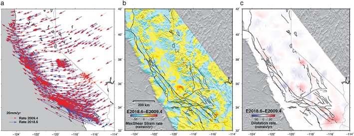
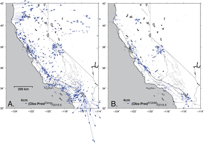
Figure 4.

Accumulated displacements and residuals (2010–2018.6): (a) Red arrows denote observed values from the Scripps Orbit and Permanent Array Center analysis, and blue arrows the predicted displacements by Zeng and Shen (2017). (b) Accumulated displacement residuals (observed‐predicted).

Figure 5.

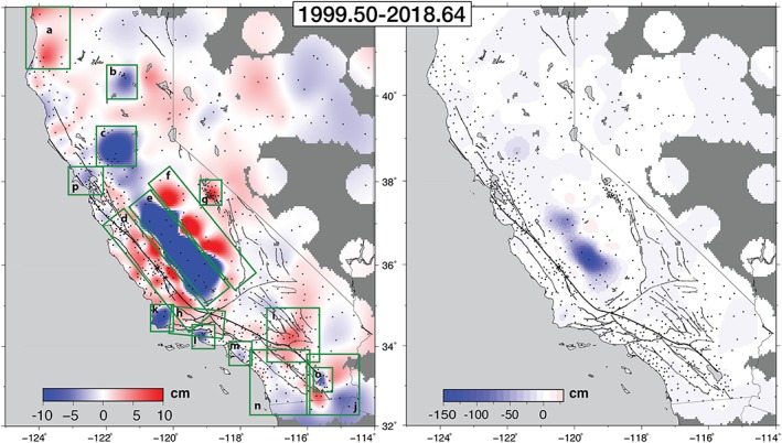
Accumulated vertical displacement field between 1999.5 and 2018.6, represented with two different color scales. See Movies S6b and S7b for a time progression of displacement fields. Refer to Table 2 for the amount of accumulated vertical motion in highlighted regions of the left panel.

The integration of the observed displacement time series and ZS2017 model is accomplished using a remove/interpolate/restore approach as follows:

1. Construct a 1‐km horizontal displacement grid at some time t after the reference epoch (for demonstration purposes we use t₀ = 2010.00) by multiplying the ZS2017 surface velocity map by t − t₀.

2. Subtract the model from the observed displacements in north and east directions at all station locations. We assume here that the residuals will be smooth so they have spatial variations at length scales greater that the spacing of the cGPS stations (>10 km).

3. Interpolate the east and north residuals (modeled minus predicted displacements) at a 1‐km grid spacing solving for 2‐D vector body forces in an elastic full space to provide coupling between the two horizontal components (Haines & Holt, 1993). This is accomplished using the GMT5 function gpsgridder (Sandwell & Wessel, 2016), where one quarter of the number of eigenfunctions are compared with the number of data points (parameter Cn); the residual grid fits the displacement residuals to within their uncertainties.

4. Add the residual grid to the ZS2017 displacement model to achieve the final horizontal displacement grids, with 1‐km spatial resolution. This defines the kinematic Geophysical‐based Model (KGbM) at any epoch t _n, KGbM(t _n), starting with KGbM(t _o) (Figure 6).

Figure 6.

Kinematic datum modeling methodology relating epoch t = 2017.7 to t ₀ = 2010 in the east component. The final upgraded weekly model (right) is the sum of the displacement field predicted by Zeng and Shen (2017; upper left) and the surface interpolation of residuals (lower left).

The final displacement grids for both north and east components are shown in Figure 7 at three different epochs. Movies S1 and S2 show the weekly residuals grids from Step 3. Movies S3 and S4 show the evolution of the final KGbM grids for the period 2010.0 to 2018.6. The number and density of cGPS stations increase quite dramatically over time as can be seen in Figure 8 and Movie S5 and can of course affect the results. We account for this by dynamically tuning the interpolation parameters as a function of the station coverage (parameter Cn; Figure 8). Note that the number and distribution of stations remain quite stable since 2009.

Figure 7.

Kinematic Geophysical‐based Model (KGbM): Surface displacements of the upgraded model in the eastward (top panels) and northward (bottom panels) components at three different epochs: (a) 2011.2, (b) 2014.2, and (c) 2018.6. All maps are represented in International Terrestrial Reference Frame 2014. See Movies S1 to S4.

Figure 8.

Interpolation parameters by year. The red curve shows the progression in the number of stations, and the blue curve the value of the gpsgridder parameter Cn (Sandwell & Wessel, 2016).

For the vertical component, weekly surface grids of cumulative displacement are directly interpolated using Green's functions for splines of the observed point displacement time series (equations (1) and (2); GMT greenspline subroutine for the scalar interpolation). This defines the Kinematic Data‐based Model, KDbM(t _n) (as compared to the geophysical model‐based KGbM) at an arbitrary epoch t _n. Figure 5 show the accumulated vertical displacement field at epoch 2018.6 with two different scales to distinguish large Central Valley subsidence from other areas of lesser magnitude and to highlight seasonal variations. Movies S6a and S7a show the evolution of accumulated vertical deformation at the two scales, starting at epoch 2010.0 (Movies S6a and S7a) and at epoch 1999.5 (Movies S6b and S7b). In both cases, when stations stop recording for several weeks or more (for maintenance or malfunction), their data are simply ignored rather than interpolate the displacements over data gaps. For stations installed later than t ₀, say at t _m, we use the grid KGbM(t _m‐1) to add the cumulative weekly displacement for the period (t _m‐1–t ₀) to the predicted position at t _m.

2.3. Weekly Velocity Changes

To distinguish time‐dependent and secular deformation, in particular postseismic, we take the derivative of the expressions for displacement equations (1) and (2),

$$\dot{y}\left(t_i\right)=\left(\widehat{b}-v_M\right)+{\sum }_{j=1}^{n_h}{h}_{j}H\left(t_i-{T_h}_j\right)+{\sum }_{j=1}^{n_k}\frac{k_j}{t_i}{e}^{\left[-\left(\frac{t_i-{T_k}_j}{{\tau }_j}\right)\right]}H\left(t_i-{T_k}_j\right)+{\epsilon }_i,$$ (4)

$$\dot{y}\left(t_i\right)=\left(\widehat{b}-v_M\right)+{\sum }_{j=1}^{n_h}{h}_{j}H\left(t_i-{T_h}_j\right)+{\sum }_{j=1}^{n_k}\frac{k_j}{{\tau }_j+t_i+T_k}H\left(t_i-{T_k}_j\right)+{\epsilon }_i,$$ (5)

and insert the estimated model parameters from the SOPAC analysis. The term v_M, the predicted surface velocity from an arbitrary fault slip model, hereafter ZS2017, is subtracted from the estimated weekly velocity. The seasonal terms in equation (1) are ignored since their amplitudes are on the millimeter level for the horizontal components, and the effect on velocity estimates is minimal over the time period (10–20 years) spanned by the displacement time series. The term ε_i recognizes that there are errors in the estimated parameters in equations (1) and (2), as well as unmodeled time‐dependent effects other than postseismic deformation, for example, subsidence bleeding into the horizontal (see assessment of horizontal vertical uncertainties in section 2.1). ZS2017 set a lower cutoff of 0.3 mm/year to avoid excessive overweighting during their fault slip inversions. However, there is no inversion performed in computing the weekly velocities (equations (4) and (5))—we are essentially computing the tangent to the time series model trace (Figure 3). We compare the displacement time series and their derivatives for station LOWS in Figure 3 for which a logarithmic model (equation (2)) is applied. Movie S8a shows the temporal and spatial evolution of the weekly velocity residuals.

2.4. Strain‐Rate and Moment Rate

The gridding methodology explained in section 2.2 is applied to the weekly residual velocity fields (Movies S9 and S10 show the interpolated residual velocity fields in north and east components) in order to evaluate time‐dependent horizontal strain rate models where the components are

$${\dot{\epsilon }}_{\mathit{ij}}=\frac{1}{2}\left(\frac{{\partial v}_i}{{\partial x}_j}+\frac{{\partial v}_j}{{\partial x}_i}\right).$$ (6)

The derivatives were calculated using the GMT5 function grdgradient, from which, we calculate the principal strain rates

$${\dot{\epsilon }}_{1,2}=\frac{{\dot{\epsilon }}_{\mathit{xx}}+{\dot{\epsilon }}_{\mathit{yy}}}{2}\pm \sqrt{{\left(\frac{{\dot{\epsilon }}_{\mathit{xx}}-{\dot{\epsilon }}_{\mathit{yy}}}{2}\right)}^2+{\dot{\epsilon }}_{\mathit{xy}}^2},$$ (7)

the maximum shear strain rate

$${\dot{\epsilon }}_{12}^{\mathit{MAX}}=\frac{{\dot{\epsilon }}_1-{\dot{\epsilon }}_2}{2}=\sqrt{{\left(\frac{{\dot{\epsilon }}_{\mathit{xx}}-{\dot{\epsilon }}_{\mathit{yy}}}{2}\right)}^2+{\dot{\epsilon }}_{\mathit{xy}}^2},$$ (8)

and the dilatation rate

$$\delta ={\dot{\epsilon }}_1+{\dot{\epsilon }}_2={\dot{\epsilon }}_{\mathit{xx}}+{\dot{\epsilon }}_{\mathit{yy}}.$$ (9)

Movies S11a and S12a show the corresponding maximum shear strain rates and dilatation rates, respectively (hereafter referred to together as “strain rates”; maximum shear strain rate is referred to as “shear strain rate”). Movies S11a and S12a show the evolution of shear strain rate and dilatation rates relative to a reference epoch 1999.5.

Due to the particular spacing of the earthquakes in this study (Table 1; Figure 1), there is little remaining postseismic motion at epochs 2009 and 2018, which allows us to assess the resolution of the strain rate fields (grids). Figure 9a shows the observed weekly velocities at these epochs, mostly showing no difference in magnitude and direction but only changes in the network over time. The strain rate differences between the two epochs are on the order of 10–20 nstrain/year in a random pattern, providing a measure of resolution for this study. Exceptions include one small pocket centered on the Salton trough showing both shear strain rate differences (Figure 9b) and diffuse extension (Figure 9c) due to long‐lasting postseismic deformation following the 2010 Mw7.2 El Mayor‐Cucapah earthquake. The Central Valley also shows a small pocket of shear strain most likely due to subsidence‐induced horizontal motion.

Figure 9.

Assessment of observed strain rate resolution. (a) Observed weekly velocities at the two epochs (2009.4 and 2018.6) not expected to have significant time‐dependent deformation. The isolated blue arrows reflect the increased station coverage between the two epochs. (b) Maximum shear strain rate differences between the two epochs; (c) Dilatation rate differences.

For a comparative analysis of the postseismic amplitude of each considered earthquake, we examine the strain rate evolution 1 week (Figure 10), 1 year (Figure 11), and 7 years (Figure 12), relative to the week prior to each event. To emphasize the larger regional context, the evolution of weekly strain rate residuals with respect to a common reference epoch t₀= 1999.78, the week prior to the 1999 Mw7.2 Hector Mine earthquake, is useful and can be found in the supporting information (Figures S1 and S2).

Figure 10.

Strain rate maps (nstrain/year) 1 week after each of the four strike‐slip earthquakes relative to the previous week. (Top) Maximum shear strain rate; (bottom) dilatation rate, red is extension and blue contraction. Dots indicate the locations of continuous Global Positioning System stations; stars, the epicenter of each event.

Figure 11.

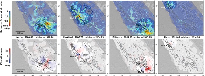
Strain rate maps (nstrain/year) 1 year after each of the four strike‐slip earthquakes relative to the week preceding the event. (Top) Maximum shear strain rate; (bottom) dilatation rate, red is extension and blue contraction. Dots indicate the locations of continuous Global Positioning System stations; stars, the epicenter of each event.

Figure 12.

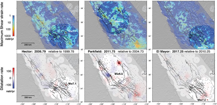
Strain rate maps (nstrain/year) 7 years after each of the three strike‐slip earthquakes relative to the week preceding the event. (Top) Maximum shear strain rate; (bottom) dilatation rate, red is extension and blue contraction. Dots indicate the locations of continuous Global Positioning System stations; stars, the epicenter of each event. The Napa earthquake is omitted since the time elapsed is less than 7 years.

Finally, to further assess the effects of postseismic deformation, we compute the moment rate (Savage & Simpson, 1997; Ward, 1998) following each earthquake:

$${\dot{M}}_0^g=2\mathit{\text{μHmax}}\left(\left|{\dot{\epsilon }}_1\right|,\left|{\dot{\epsilon }}_2\right|,\left|{\dot{\epsilon }}_1+{\dot{\epsilon }}_2\right|\right)\mathit{dA},$$ (10)

where dA is the size of the elementary cell resolution (1 × 1 km), H is the faulting depth, and μ is the shear modulus. For a given event, we then integrate ${\dot{M}}_0^g$ over its region of impact and estimate the accumulated postseismic moment over a specific period. We use an average faulting depth of 15 km for all strike‐slip events and a faulting depth of 30‐km depth for thrust events in the Cascadia subduction zone. Postseismic moment rates and equivalent moment magnitudes are gathered in Table 3, along with the corresponding area and time period.

Table 3.

Estimated Postseismic Moment Release

Region	Zone	Reference epoch	Period	Cum. Moment (N·m)	Mw	Type of deformation
Southern California (ECFZ)	116–118°W 22.5–4.5°N	1999.79	1999.79–2003.95	2.6·1018 (H = 15 km)	6.2	Postseismic Hector Mine earthquake
Central SAF	120.3–122°W 35–36.5°N	2003.96	2003.96–2018.6	9.6·1018 (H = 15 km)	6.6	Postseismic San Simeon and Parkfield earthquakes
Central SAF	120.3–122°W 35–36.5°N	2003.96	2003.96–2004.74	1.7·1018 (H = 15 km)	6.1	Postseismic San Simeon earthquake
Southern segment of SAF, Imperial Fault	114.5–116.5°W 32–33.5°N	2010.25	2010.27–2018.6	1.1·1019 (H = 15 km)	6.6	Postseismic El Mayor‐Cucapah earthquake
San Francisco Bay area	121.5–122.5°W 37–38.5°N	2014.64	2014.65–2018.6	3.9·1017 (H = 15 km)	5.6	Postseismic Napa earthquake
Northern California, Cascadia 1	123–124°W 41–42°N	Ø	2005.00–2018.6	8.2·1018 (H = 30 km)	6.5	Misfita interseismic + postseismic 2005 Gorda and 2010 Eureka earthquakes
Northern California, Cascadia 2	123–124°W 40–41°N	Ø	2005.00–2018.6	5.2·1018 (H = 30 km)	6.4	Misfita interseismic + postseismic 2010 Eureka earthquake

Note. ECFZ = Eastern California Shear Zone; SAF = San Andreas Fault.

^aMisfit compared to 2‐D secular fault slip model of Zeng and Shen (2017).

3. Transient and Secular Discrepancies

In this section, we highlight by region the horizontal spatiotemporal features that are not well captured in the secular ZS2017 model, including transients and secular motions. We also identify transient and secular vertical displacements, without the adoption of a background vertical motion model. This serves as a basis for maintaining a 3‐D kinematic reference frame as a geodetic datum for surveying and precise geographic information systems by assimilating both secular and transient motions in a timely manner and making adjustments when necessary, for example, after a significant earthquake.

3.1. Southern California

3.1.1. Postseismic Motions

Two major earthquakes occurred over the period of our observations, the 1999 Mw7.1 Hector Mine and the 2010 Mw7.2 El Mayor‐Cucapah earthquakes (Table 1). The distribution of cGPS stations for the former event is limited to the west of the rupture zone. For the latter, the closest stations are ~50 km to the north of the epicenter. Both earthquakes caused significant permanent displacements throughout southern California.

The surface expression of the postseismic deformation in the week following the Hector Mine earthquake reveals maximum shear strain rates of about 200 nstrain/year in a 50‐km‐wide region encompassing the Eastern California Shear Zone (ECFZ; Figure 10), although it might be an underestimate because of the network coverage at the time. Areas of shear strain rate reaching 100 nstrain/year are observed northwest of the SAF, in the greater Los Angeles region and across the San Jacinto fault, within a radius of ~250 km. A lobe of contraction reaching 100 nstrain/year is observed ~50 km west of the rupture zone. In contrast, extension of the same order of magnitude is observed in the Los Angeles Basin and across the San Jacinto fault. Within a year and with the increase of the number of cGPS stations, the area of shear strain rate has significantly diminished but still reaches 350 nstrain/year (Figure 11) in the epicentral region. The dilatation rates have diminished to below 90 nstrain/year in the lobe of contraction, with the zone of extension shifting northward to cover the San Jacinto fault area up to the epicentral region, perhaps due to the increase in the number of stations. The strain rates are negligible (below the resolution level) by 3 years after the event (Figures S1 and S2; Movies S11a and S12a).

The week following the 2010 El Mayor‐Cucapah earthquake shows strain rate perturbations up to 400 nstrain/year centered in the Imperial Valley between the SAF and the San Jacinto faults up to the Salton Sea (Figure 10) and extending into the ECFZ. There is a significant zone of extension (~300 nstrain/year) normal to the Salton trough and across the SAF, San Jacinto, and Elsinore faults (Figure 10). Contraction smaller than 100 nstrain/year is observed to the northwest throughout adjacent San Diego County including the Elsinore fault. There are two zones of extension up to the northern end of the San Jacinto fault and in the ECFZ. One year after the event (Figure 11) to 4.5 years (at Epoch 2014.66; Movies S11a and S12a), significant shear strain and dilatation rates below 100 nstrain/year are still observed in a more limited area across the Salton trough and Imperial fault zone. The postseismic strain rates for the El Mayor‐Cucapah earthquake have drastically diminished by 7 years after the event (Figure 12).

3.1.2. Tectonic and Anthropogenic Vertical Motion

Before 2010, we see large‐scale subsidence across southern California with the exception of the region around the 1999 Hector Mine earthquake, which is uplifting at least until the 2010 El Mayor‐Cucapah earthquake (~10 years; Movie S6a). Following the El Mayor‐Cucapah earthquake, the southern terminus of the SAF system experiences until the end of our measurements (~8 years) a persistent broad‐scale postseismic vertical motion over a region of ~400 km including two lobes of uplift (reaching 70 mm; Table 2, Region j) on a northeast to southwest axis running just south of the Salton Sea. We also observe two orthogonal lobes of subsidence on a southeast to northwest axis. The northwest lobe is located in the Salton trough, which experienced two episodes of earthquake swarms in the period of our observations, up to Mw 5.1 in 2005 (Obsidian Butte swarm; Lohman & McGuire, 2007) and Mw5.3‐5.5 in 2012 (Table 1). There we measure at several cGPS stations up to 75 mm of subsidence between 1999.5 and 2018.6 (Figure 13) most likely due to the Salton Sea Geothermal Field, an area of fluid injection and extraction (Eneva et al., 2009). The 2012 swarms may have been triggered by aseismic slip on a shallow normal fault beneath the geothermal fields that was initiated in 2010 when the injection rate rapidly increased (Wei et al., 2015).

Table 2.

Cumulative Vertical Displacements Estimated Between 1999.5–2018.6 and 2010–2018.6

Area	Cumulative displacement 1999.5–2018	Cumulative displacement 2010–2018	Source
a. Cascadia Subduction	+80 mm	+70 mm	Tectonic
b. Mount Lassen	−70 mm	−60mm	Magmatic
c. Sacramento Valley	−225 mm	−190 mm	Tectonic
d. Coastal Ranges	+90 mm	+25 mm	Tectonic
e. Central Valley	−1700 mm	−1150 mm	Groundwater pumping + drought
f. Sierra Nevada Ranges	+160 mm	+120 mm	Tectonic
g. Long Valley Caldera	+90 mm	+90 mm	Magmatic
h. Transverse Ranges	+50 mm	+25 mm	Tectonic
i. Eastern California Shear Zone	+60 mm	+25 mm	1999 Mw7.1 Hector Mine postseismic
j. Southern terminus SAF system	−20mm (SE)/+70 mm	−10 mm (SE)/+60 mm	2010 Mw7.2 El Mayor‐Cucapah postseismic
k. Santa Maria Basin	−120 mm	−140mm	Groundwater pumping
l. Ventura Basin	−70 mm	−45 mm	Tectonic/Groundwater pumping
m. Los Angeles/Santa Ana basin	−20mm	−35mm	Groundwater pumping
n. Southern California	−22mm	−27mm	Tectonic
o. South of Salton Sea	−75mm	−70mm	Salton Sea Geothermal Field
p. North San Francisco Bay Area	−45mm	−25mm	Tectonic/Groundwater pumping
q. Northern Basin and Range	±30mm	±25mm	Tectonic

Figure 13.

Kinematic datum (Kinematic Data‐based Model) accumulated vertical displacement fields showing seasonal and anthropogenic deformation between 1999.5 and four different epochs: (a) 2005.01, (b) 2010.00, (c) 2015.01, and (d) 2018.6. See Movies S6b for a time progression of displacement fields.

A broad zone of subsidence (more than 20 mm of displacement over 18.6 years) is visible to the west of the Elsinore fault extending to the coast in San Diego County (Figure 5, 6, 7, 8, 9, 10, 11, 12, 13; Table 2, Region n). This may be related to features in the data seen in previous studies that have attributed vertical motion of ±2 mm/year over a 200‐km region at the terminus of the SAF system to a crustal deformation cycle with a viscoelastic component (Smith‐Konter et al., 2014). The model including long‐term tide gauge predicts uplift and subsidence consistent with far‐field flexure due to more than 300 years of fault locking and creeping depth variability (Howell et al., 2016). However, the pattern of long‐term secular motion of order ±2 mm/year that they attribute to the earthquake loading cycle may be limited to the observed postseismic period.

3.2. Western Transverse Ranges

3.2.1. Secular Horizontal Motion

We see small differences in residual shear strain rates of ~20 nstrain/year across the Santa Barbara Channel (Figure 14b) and increasing north‐south contraction of ~20–50 nstrain/year north, across the Western Transverse Ranges (Figure 1), including the Ventura and Los Angeles basins (Figure 14c). This region represents a complex active fault system with east‐west trending oblique reverse faults and folds with primarily N‐S shortening (~10 mm/year; Marshall et al., 2013; Shaw & Suppe, 1994). The Ventura and Santa Maria basins are areas at risk of a seismic event of order Mw7.5–8.0 (McAuliffe et al., 2015). The Santa Barbara channel is intersected by a series of active east‐west trending thrust and normal faults including the western extent of the Ventura basin (Donnellan et al., 1993; Shaw & Suppe, 1994) with about 4–5 mm/year velocities south‐south east with respect to the Channel Islands (Shen et al., 2011). Since we are interpolating strain rate from surface observations, we cannot distinguish faults that are the source of the observed discrepancies, but the residual strain rates should be considered in the assessment of seismic risk in this area. The Los Angeles basin is also intersected by a complex fault system with significant shortening (Shen et al., 1996; Walls et al., 1998). The velocity residuals of ~1 mm/year are consistent with more contraction across the basin (Movie S8b).

Figure 14.

Residual maps and grids. (a) Velocity residual map (observed minus ZS2017‐predicted); (b) maximum shear strain rate residual grids; (c) dilatation rate residual grids at epoch 2018.59. Red vectors indicate extension; blue vectors indicate contraction. Areas of interest described in the text are indicated by red dashed boxes including magnitudes. Values of strain rate are indicated for each area highlighted by a red contour. When important variations are observed, we give both the mean and the maximum values (“mean/max”). For areas where strain rate is homogeneous, only the mean value is indicated.

3.2.2. Anthropogenic Subsidence

The Los Angeles basin and the Santa Ana basin to the southeast (Figure 1) also experience well‐documented anthropogenic subsidence from groundwater pumping, aquifer recharge, and oil pumping (Argus et al., 1999; Bawden et al., 2001; Lanari et al., 2004; Watson et al., 2002) (Figure 5 – Region m), which likely bleeds into the horizontal velocities. We observe contiguously in the two basins (Figure 5, Region m) an accumulated subsidence (over 19 years) of ~20 mm. From a combination of cGPS and InSAR data from 1997–1999, just prior to the start of our displacement time series, Bawden et al. (2001) found about 12 mm/year of subsidence with seasonal variations of up to 55 mm. A later analysis with InSAR data from 1995–2002 showed line‐of‐sight (LOS) average velocities of −3 up to −10 mm/year in the Santa Ana basin (Lanari et al., 2004). We also see subsidence (Table 2) in the Oxnard Plain in coastal Ventura County and the Ventura basin (Figure 5, Region l) due to a combination of tectonic movement, hydrocarbon extraction, and groundwater pumping (Colesanti et al., 2003; Donnellan et al., 1993; Hanson et al., 2003). Note that the measured Santa Maria subsidence of ~120 mm is due to a single cGPS station (Region k, Figure 5; Table 2) but appears to be a real effect.

3.3. Central California and the Bay Area

3.3.1. Postseismic Motions

The 2003 Mw6.5 San Simeon earthquake that occurred on a blind thrust in the Coast Ranges generated significant postseismic deformation, ~2,000 nstrain/year in near field and over 500 nstrain/year at distances of ~150 km. About 100 nstrain/year was observed from the Channel Islands up to the San Francisco Bay area, with some gaps in between due to limited station coverage (supporting information: Figures S1 and S2; Movies S11a and S12a). The postseismic response largely dissipated by 2004.73, that is, just before the 2004 Mw6.0 Parkfield earthquake (Movie S11a and S11b).

The Parkfield earthquake triggered stronger postseismic perturbations in the near‐epicentral region, of several thousands of nstrain per year in shear strain rate despite its lesser moment magnitude, to about 100 nstrain/year over a larger area than that of the San Simeon event (Figure 10). The pattern of alternating extension and contraction, centered on the epicenter, is consistent with shallow and heterogeneous fault processes, although the station coverage could certainly create some artifacts. One year later, the strain rate deviations have dramatically decreased, implying a rapid relaxation (Figure 11). The same dilatation rate pattern is visible with better station coverage supporting a real process, but with a significantly lesser amplitude below 100 nstrain/year. After 7 years, the postseismic effects of the 2004 Parkfield event have mostly dissipated although we still observe a small lingering shear strain rate in the region (Figure 12).

By comparison, the postseismic deformation following the 2014 Mw6.0 Napa earthquake, although having the same magnitude as the 2004 Parkfield event, has a very weak amplitude over the first weeks (epoch 2014.66; Figure 10). The strain rate barely reaches 200 nstrain/year over a limited area, less than 100 km from the epicenter. Some extension is observed in the vicinity of the epicentral region with a broader zone of compression to the east with a half‐ring pattern. One year after the event, we observe less than 50 nstrain/year (Figure 11) compared to more than 350 nstrain/year over a significantly larger area for the 2004 Parkfield event. The postseismic deformation has largely dissipated within 3 years after the event (Movies S11a and S11b).

3.3.2. Accelerated Fault Creep

Although quite dense in the Bay Area, station coverage was very sparse in the Parkfield region with only a small scale (region of about 25 × 25 km) network installed in 2003 (Langbein & Bock, 2004). No significant strain rate transients can be observed from 1999 to the 2003 San Simeon earthquake (Movie S11a). Both the San Simeon and Parkfield earthquakes increased the shear strain rate from the epicentral region to the San Francisco Bay Area although very few stations were in operation between the two regions (see red rectangle in Figure 14). For both earthquakes, the postseismic transient became insignificant within 9–12 months of the respective event. However, at ~2006.7, there is a significant increase to 30–70 nstrain/year in this area that persists to 2018.6. The most straightforward explanation is an increase in the creep rate above the background rate along the SAF into the Calaveras fault (Simpson et al., 2001) at its bifurcation with the SAF. Accelerated creep has also been documented by alignment arrays and creepmeters (Lienkaemper et al., 2006) in the SAF creeping section in central California, as well as short‐term transient creep (“silent slip”) events across the SAF system in southern California (Wei et al., 2009; Wei et al., 2011). Our result indicates a creep transient that has persisted for more than a decade after the 2004 Parkfield earthquake, which corroborates a long‐term accelerated creep transient of ~6–12 years observed after the event (Lienkaemper & McFarland, 2017). In addition, using GPS and InSAR data collected over this region from 1992 to 2010, Khoshmanesh and Shirzaei (2018) identified intermediate‐term creep rate variations that evolve over a decadal scale.

3.3.3. Orogenic Uplift

In the Sierra Nevada to the east of the Central Valley (Region f, Figure 5), our analysis identifies a region of significant uplift between 2010 and 2018.6, reaching a total displacement of 12 cm in the northwest and a broad area of lesser uplift to the southeast, which is consistent with the results of (Hammond et al., 2016) based on 5–20 years of GPS data up to 2016. On the western side of the Central Valley (Region d, Figure 5), we see about 90 mm of uplift along the Coast Ranges, also consistent with Hammond et al. (2016). In comparison there is uplift of about 50 mm in the Transverse ranges (Table 2, Region h) consistent with Hammond et al. (2018).

3.3.4. Subsidence and Drought

California's Central Valley is a prototypical example of severe anthropogenic subsidence. It is bounded by the Sierra Nevada to the east and the Coast Ranges to the west, with an area of about 52,000 km² and is divided by the Sacramento‐San Joaquin river delta into the San Joaquin Valley to the south and the Sacramento Valley to the north. Both areas experience significant subsidence due to groundwater extraction for agricultural development causing downward motion due to soil compaction, while upward motion occurs when aquifers are recharged. Vertical land motion also results from the solid Earth's elastic response to the loading and unloading of snow and surface water. Therefore, drought conditions will result in vertical uplift due to the loss of surface and near‐surface water mass (Amos et al., 2014; Argus et al., 2014; Argus et al., 2017; Borsa et al., 2014). However, there was increased groundwater extraction in the San Joaquin Valley during the drought between 2012 and 2017 causing net subsidence.

A critical mass of cGPS stations became available in the San Joaquin Valley in 2005 (Figure 1; Movie S5) from the PBO network and the Central Valley Spatial Reference Network operated by the California Department of Transportation. The accumulated vertical displacement field (Figure 5; Table 2, Region e) is shown at two different scales to distinguish Central Valley subsidence from other areas of lesser magnitude, as well as seasonal variations (Movies S6a and S6b). With the onset of the drought in 2012, there is a significant increase in the rate of subsidence from 2012 until the end of 2017, with a total displacement of 1.7 m (see Figure 2 for stations LEMA and CRCN). This is consistent with increased groundwater pumping due to a combination of decreased surface‐water availability and land use changes (Faunt et al., 2016). The effects of aquifer changes in the Sacramento Valley result are only about 0.2 m of subsidence (Figure 5; Table 2, Region c), somewhat less than found in a USGS study (https://pubs.usgs.gov/fs/2000/fs00500/pdf/fs00500.pdf). However, this area is not well covered with cGPS stations, and our result may be biased by a single station on Sutter Buttes (station SUTB), an eroded volcanic lava domes that is the highest point in the Central Valley (~700 m), which is not significantly subsiding. After 2017, the rate of subsidence dramatically decreases, primarily due to heavy precipitation in early 2017, but increases again with continued groundwater pumping toward the end of 2017 and continues until 2018.6, the end of our observations.

3.4. Northern California

3.4.1. Transition From Transform to Thrust Faulting

Northern California is characterized by a complex transition from transform to variably coupled thrust faulting. Unfortunately, the sparsity of cGPS stations prevents us from performing any analysis before 2005, which marks the beginnings of the PBO network. Between 2005 and 2018.6, we observe significant east‐north east velocity differences ranging from 7 to 14 mm/year, resulting in 30 to 70 nstrain/year both in dilatation and shear strain rates (Figure 14). Two distinct areas are visible. First, the southern part (between 40°N and 41°N) is deforming due to both Cascadia subduction and the complex tectonics of the Mendocino Triple Junction where we observe between 30 and 70 nstrain/year, with a possible contribution of on‐land deformation of the Rogers Creek‐Maacama fault zone. Second, the northernmost part (between 41°N and 42°N) is predominately driven by subduction with residual strain rates of order 30 nstrain/year (Figure 14c).

Over the period considered, three significant thrust earthquakes occurred offshore on the Gorda plate (Figure 1), in 2005 Mw7.2, 2010 Mw6.5, and 2014 Mw6.9, which affected a small number of cGPS stations. Due to the absence of very large subduction earthquakes over the last several decades with expected large‐scale and long‐lasting viscoelastic relaxation, we attribute the observed strain rate residuals to limitations in the secular ZS2017 model. They defined three tectonic blocks in northern California, the narrow coastal Rogers Creek‐Maacama fault zone block; the parallel, narrow inland Bartlett Springs‐Green Valley block; and the oceanic Gorda‐Juan de Fuca block, the locus of the Cascadia subduction zone, which they modeled using an elastic dislocation (back slip) model (Savage, 1983). The entire subduction zone was divided into 17 downdip slabs with three slabs at the convergent boundary along the Gorda plate. Although it provides a reasonable fit at the regional scale over Western North America, the constant slip rate attributed to each downdip slab may still be a too simple assumption to reproduce the potentially highly variable coupling pattern along the fault interface, where regular transient slip events associated with tremor activities are also occurring (Pollitz & Evans, 2017; Rogers & Dragert, 2003).

We tested simple back slip forward models (Savage, 1983) to verify if the magnitude of velocity and strain rate residuals could be explained by inaccurate parameters defined by ZS2017 along the Cascadia subduction zone. By taking a reasonable range of input parameters controlling the fault geometry from the 2008 National Seismic Hazard Map Project (Peterson et al., 2008), we find that small changes in dip angle, slab width, or slip rate can considerably affect surface strain rates by tens of nstrain per year. The higher amplitude of strain rate residuals (up to ~70 nstrain/year) observed onshore of the Mendocino Triple Junction is consistent with more complex fault interactions, and the observed velocities most likely align with the actual convergence direction at a rate ranging from 30 to 35 mm/year at these latitudes.

3.4.2. Vertical Secular Motion

A Cascadia 3‐D dislocation model using long‐term tide gauge data predicts 1–2 mm/year uplift from the Mendocino Triple Junction (Cape Mendocino) to the Oregon border (Wang et al., 2003), consistent with tidal and leveling records (Burgette et al., 2009). An analysis of GPS data up to 2015 in southern Cascadia shows uplift averaging 1–2 mm/year, with a maximum near 4 mm/year just south of the Oregon border (Crescent City), and dropping to zero at Cape Mendocino (Montillet et al., 2018). We see a more nuanced picture with two clear lobes of uniform uplift, a total displacement reaching 80 mm centered on 41°N latitude up to ~100 km from the coast decreasing to 10 mm at the Mendocino Triple Junction up to ~50 km from the coast (Figure 5; Table 2, Region a; Figure 13).

3.5. Northern Basin and Range

3.5.1. Secular Horizontal Motion

The Northern Basin and Range is dominated by east‐west extension about north striking normal faults and northwest‐directed right‐lateral shear on a complex system of strike slip, normal and detachment faults with extensive sGPS and cGPS measurements and analysis (e.g., Bennett et al., 2003; Hammond et al., 2014). Although not a focus of our kinematic datum study in California, we observe coherent velocity residuals with a magnitude of ~1 mm/year directed east to southeast in the Northern Basin and Range province (Figure 14) about an order of magnitude less than the observed surface velocities and opposite to the known direction (Figure 14a). (The Basin and Range velocities have the lowest uncertainties of the data set [0.05–0.1 mm/year] primarily due to the dry desert conditions and stable monumentation; Davis et al., 2003.) Our observations imply that the ZS2017 model slightly overestimates fault slip rates, indicating less extension and less right‐lateral shear. Further north across Nevada, the residual velocities are coherent in a northwesterly direction with a magnitude of order 3 mm/year. This is somewhat consistent in direction with the rotation of the northwestern United States, which extends to southern Cascadia and the Northern Basin and Range (McCaffrey et al., 2013).

3.5.2. Secular Vertical Motion

We observe alternating broad zones of secular uplift and subsidence in the Northern Basin of Range across Nevada into northern California of order ±25–30 mm over 19 years (Figures 5 and 13; Table 2, Region q). Gourmelen and Amelung (2005) used InSAR measurements (from 1992 to 2000) near the rupture zone of two normal and two strike‐slip earthquakes (M6.8 to M7.3) in Nevada from 1915 to 1954. They detected a broad area of 2–3 mm/year uplift that can be explained by postseismic mantle relaxation. This is larger than our average of ~1–1.5 mm/year of uplift in the same area over 19 years consistent with continued but perhaps diminishing postseismic relaxation. Note that we also observe a more limited region of subsidence of the same order of magnitude to the southwest of the Gourmelen and Amelung (2005) study area, as well as a broader region to the east. The uplift and subsidence appear not to be correlated with topography; during earthquakes, the basins drop, but the ranges show little or no rise (Thompson & Parsons, 2016).

3.6. Magmatic Deformation

Magmatic inflation at Long Valley Caldera (Figure 1) is a good example of vertical motion bleeding into significant horizontal displacements, in this case, radiating away from the source. The Long Valley Caldera has been monitored with geodetic methods for several decades (Dixon et al., 1997). At Long Valley Caldera, an inflation event occurring between 2011 and end of 2018 generated about 90 mm of uplift (Table 2, Region g), as well as transient horizontal motion of about 10 mm in both components, superimposed on the long‐term trend (Figure 2), consistent with Montgomery‐Brown et al. (2015) from GPS and InSAR measurements. In 10 years, we observe a cumulative horizontal displacement of more than 50 mm radiating in all directions (Figure 4). Mount Lassen (Lassen Peak) an active volcano in California has been monitored by cGPS starting in 2008 as part of the PBO network. Here we observe subsidence of about 70 mm since the start of monitoring in 2006 (Figure 5, Region b), consistent with other studies (Dzurisin, 1999; Hammond et al., 2016; Parker et al., 2016), and corresponding radial horizontal displacements, about 50% smaller (Figure 4).

4. Postseismic Comparison and Moment Rates

In this section, we compare the short‐ to long‐term characteristic motions of the earthquakes with significant postseismic deformation (Table 1) and calculate their respective moment rates (equation (10); Figure 15; Table 2). We first discuss the four strike‐slip earthquakes in southern and central California and then the Gorda plate thrust events in Cascadia.

Figure 15.

Postseismic moment rate evolution as function of time for the eight earthquakes of this study: Parkfield region (red), Bay Area (green), Southern California (blue), Cascadia (black), and Central California (cyan). Refer to Table 3 for equivalent moment magnitudes. SAF = San Andreas Fault.

4.1. Strike‐Slip Events

A comparison of the short‐ to long‐term spatiotemporal postseismic characteristics of the four strike‐slip earthquakes (Table 1; Figures 10, 11, 12) at representative stations is presented in Figure 16 after normalizing the horizontal displacement time series by their respective coseismic offsets. We are motivated by Trubienko et al. (2014) who noticed that this metric increases with distance to the trench with almost constant value for a range of distances for three great subduction earthquakes, providing insight into the role of various rheological and geometrical parameters.

Figure 16.

Postseismic horizontal displacements normalized by coseismic displacements for representative stations located in the regions of the 1999 Hector Mine, 2004 Parkfield, 2010 El Mayor‐Cucapah, and 2014 Napa earthquakes, as function of time since the earthquake (0 = date of the earthquake). The red dashed lines highlight the epochs considered in Figure 10 (1 week), 11 (1 year), and 12 (7 years). Locations of stations are shown in Figure S3.

4.1.1. Southern California

Both the 1999 Mw7.1 Hector Mine and 2010 Mw7.2 El Mayor‐Cucapah earthquakes caused widespread postseismic displacements over most of southern California. The duration and spatial extent of postseismic deformation are important in assessing the dominant underlying processes.

We observe a longer duration of postseismic motion for the 2010 Mw7.2 El Mayor‐Cucapah earthquake (~7 years) compared to 1999 Mw7.1 Hector Mine earthquake (~3 years; Figure 16). For Hector Mine, the postseismic/coseismic ratio converges rapidly to two units at 1–2 years after the event, with a single station (MSOB) converging to three units after about 5 years. On the other hand, for El Mayor‐Cucapah, the ratio gradually increases over time, not yet reaching a plateau even after 7 years. Both events involve complex rupture of several faults (e.g., Gonzalez‐Ortega et al., 2014; Simons et al., 2002). However, Hector Mine has a 20‐km depth compared to 6 km for El Mayor‐Cucapah—the estimated decay times are 183 and 283 days, respectively. Note that one station shows an even larger postseismic to coseismic ratio for the 2010 event (P496), with a somewhat constant southeastern slope approaching four units by the end of the time series (2018.6). The station is at the southern end of the right‐lateral strike‐slip Wienert fault, the southeastern extension of the Superstition Hills fault zone that ruptured in 1987 (Hudnut et al., 1989). This area is known to experience episodic shallow surface creep (e.g., Bilham & Behr, 1992; Wei et al., 2009). Multiple faults in the Imperial fault zone, including the Wienert fault, experienced shallow‐triggered slip after the El Mayor‐Cucapah earthquake as documented by InSAR and creepmeters (Wei et al., 2011). In the case of P496, the larger‐scale postseismic deformation appears to be modulated by triggered slip, which continues at least until the end of the time series (2018.6).

Postseismic models of the 2010 event are varied; some studies favor fault afterslip processes (Gonzalez‐Ortega et al., 2014), while others favor deep mantle processes (Pollitz et al., 2012), (Dickinson‐Lovell et al., 2017). In the first study, short‐term and near‐field high‐resolution InSAR imagery and GPS data were used, allowing to precisely image the fault processes, but with limited far‐field coverage. After ~8 years, accumulated postseismic moment for the El Mayor‐Cucapah earthquake is about 1.1 × 10¹⁹ N·m, equivalent to an Mw6.6 earthquake (Table 3, using H = 15‐km depth), which is larger than previous estimates based on the first 6 months following the event (Gonzalez‐Ortega et al., 2014). For the Hector Mine earthquake, the accumulated moment over this period reaches 2.6 × 10¹⁸ N·m, equivalent to an Mw6.2 earthquake. Table 3 also indicates postseismic moment release for a 10‐km depth. Based on near‐field InSAR measurements, Jacobs et al. (2002) infer a postseismic moment on the order of 10¹⁸ N·m.

Long‐lasting viscoelastic relaxation, in our case on a continental strike‐slip fault, can also generate increasing stress and induce failure on neighboring segments (e.g., Yang & Toksöz, 1981) further complicating seismic risk assessment. This was hypothesized for the 1992 Mw7.3 Landers earthquake, also in the ECFZ, which may have triggered the 1999 Hector Mine event, (e.g., Freed & Lin, 2001).

4.1.2. Central California

The strain rate fields over the first week following the 2004 Mw6.0 Parkfield earthquake (Figure 11) are dramatically larger than any other of the strike‐slip events observed in California between 1999 and 2018 (Table 1). This exceptionally large postseismic deformation over the first weeks to months has been observed in earlier studies of the Parkfield event focused on coseismic and postseismic slip (e.g., Bruhat et al., 2011). The normalized displacements clearly show very strong and rapid postseismic motion with a postseismic/coseismic ratio flattening to two to three units by about 7 years, which is consistent with the progression of the residual strain rate fields (Figures 10, 11, 12). This difference of amplitude between this event and the 2014 Mw6.0 Napa earthquake (of the same magnitude) is quite striking, and directly visible on the normalized displacement time series (Figure 16).

The calculation of the postseismic moment release for the Mw6.5 San Simeon and 2004 Mw6.0 Parkfield earthquakes is complicated by their proximity (50 km) and the short 0.75‐year interval between the two events (Figure 1). For the San Simeon event, we calculate a moment release of up to 1.7 × 10¹⁸ N·m, considering a seismogenic depth of 15 km, which is equivalent to a Mw6.1 earthquake just prior to the Parkfield event. Similarly, based on InSAR and GPS measurements, a lower bound on postseismic moment release for the San Simeon event was estimated to be 1.16 × 10¹⁸ N·m (Mw6.0; Johanson & Bürgmann, 2010). Our cGPS observations are limited to the epicentral region of the San Simeon and Parkfield events with very few stations to the north of both ruptures. Nevertheless, an examination of the far‐field strain rates a week prior to the Parkfield event (Figure 10) indicates that the remaining postseismic transient is negligible. Regardless, we estimate the combined postseismic moment for both the San Simeon and the Parkfield earthquake to be 9.6 × 10¹⁸ N·m (equivalent Mw6.6) for a 15‐km depth. Considering the lesser moment accumulated over the first months by the San Simeon event (Table 2), we can conclude that the postseismic moment release due to the Parkfield event is significantly larger than the earthquake itself, consistent with previous studies (Murray & Langbein, 2006). After investigating the three main mechanisms (afterslip, viscoelastic relaxation, and poroelastic rebound), Freed (2007) concluded that afterslip was solely responsible for the postseismic deformation. Furthermore, several studies postulate that the postseismic deformation is a lower crust process and consistent with velocity strengthening friction (Barbot et al., 2009; Bruhat et al., 2011; Johanson et al., 2006). In comparison, the postseismic release for the 2014 Mw6.0 Napa earthquake is only 3.9 × 10¹⁷ N·m (equivalent Mw5.6) over 3 years (Table 2) assuming a 10‐km depth. This is somewhat inconsistent with the result that moment release was mostly postseismic after the event (Lienkaemper et al., 2016).

In forming weekly displacement time series, we realize that we have smeared out coseismic motion into the immediate postseismic period. We indeed chose not to use daily displacements or divide the data into two segments, one pre‐earthquake and one post‐earthquake. Nevertheless, to test the effect of weekly versus daily sampling, we investigated the first few days after the Parkfield earthquake, which triggered postseismic deformation with the largest displacement gradients. The postseismic moment release did not significantly differ.

4.2. Gorda plate thrust earthquakes

The Mw6.7 and Mw7.2 Gorda plate earthquake sequence on 15–16 June 2005 had limited on‐shore surface expression due to the sparseness of stations and dissipated within ~18 months (Movie S8a), with an estimated exponential decay time of about 243 days. Similarly, the 2010 Mw6.5 Gorda plate earthquake had limited on‐shore spatial extent and dissipated within about 6 months, with an exponential decay of about 50 days (Table 1). The 2014 Mw6.9 Gorda plate event generated no visible postseismic motion. We identified two distinct areas of residual displacements for the 2005 events. First, the southern part (between 40°N and 41°N) is deforming due to both Cascadia subduction and the complex tectonics of the Mendocino Triple Junction where we observe between 30 and 70 nstrain/year, and a possible contribution to on‐land deformation of the Rogers Creek‐Maacama fault zone. Second, the northernmost part (between 41°N and 42°N) is predominately driven by subduction with residual strain rates of order 30 nstrain/year (Figure 14c).

We estimate an accumulated moment up to 5.2 × 10¹⁸ N·m in the lower region (equivalent Mw6.4), slightly larger in the northern region (equivalent to Mw6.5 earthquake; Table 3) for a seismogenic depth of 30 km. Since there is no major earthquake, these values mostly account for the overall moment accumulation due to the interseismic model misfit. These appear to be insignificant numbers to affect seismic risk (Melbourne et al., 2002). However, the moment release rate of a deep episodic tremor and slip (ETS) event, which frequently occurs in the southern Cascadia region, is significantly smaller (e.g., Aguiar et al., 2009) but may trigger large subduction zone earthquakes such as the 2011 Mw9.0 Tohoku‐oki earthquake (e.g., Ito et al., 2013). To put this into perspective, damage and death from a great earthquake on the Cascadia megathrust and subsequent tsunami (with a recurrence time of about 300 years and the last one in 1700; Atwater & Hemphill‐Haley, 1997; Satake et al., 1996) are likely to be comparable to the 2011 Mw9.0 Tohoku‐oki event (Goldfinger et al., 2003).

5. Applications

5.1. Kinematic Datum

A kinematic datum is a critical resource for the different communities using precise GNSS positioning and spatial referencing in major continental fault zones, such as the Western United States. Having a large portion of California moving at tens of millimeters per year with respect to stable North America, punctuated by 19 significant earthquakes since 1992, as well as postseismic deformation for eight of the events (Table 1) poses a significant problem. The current practice is to periodically define a new reference frame based on a set of estimated cGPS station coordinates and velocities at a particular epoch of time. This is similar to the approach for global reference frames that rely on the trajectory of station positions (Altamimi et al., 2017; Bevis & Brown, 2014) and a methodology to provide a 2‐D regional model for precise positioning applications in active tectonic environments (Pearson & Snay, 2013). In California, for example, a new epoch at 2017.50 was recently published by the California Spatial Reference Center (CSRC; Bock et al., 2018; http://sopac-csrc.ucsd.edu/index.php/epoch2017/), replacing the previous Epoch 2011.00. There have been five previous epoch dates published since 2000.35 (http://sopac-csrc.ucsd.edu/index.php/previous-datums/).

The kinematic datum provides the transformation from three‐dimensional coordinates at an arbitrary epoch date to another at any location within California, using the extensive network of cGPS stations (Bock et al., 2018; http://sopac-csrc.ucsd.edu/index.php/epoch2017/). Referring to section 2.2, to transform the horizontal coordinates of a point surveyed at epoch t _n back to epoch t _m, we simply apply a grid correction KGbM(t _m) minus KGbM(t _n), where KGbM(t _m) contains the cumulative displacements from t ₀ to t _m and KGbM(t _n) the cumulative displacements from t ₀ to t _n (Figure 17); similarly, we use KDbM for the vertical component. As an example, Figure 18 shows the residual displacements at the cGPS stations before and after applying the kinematic datum horizontal grid corrections on the last week of our data set, that is, KGbM(t = 2018.65). The gridded residuals for the horizontal KGbM(t _n) and vertical KDbM(t _n) weekly grids then represent the weekly misfit grids for the horizontal (Figure 19) and vertical (Figure 20) corrections, respectively. Movies S13 and S14 show the evolution of the weekly misfit grids for the horizontal components from t ₀ = 2010 to t = 2018.65. Movies S15a and S15b show the vertical misfits from t ₀ = 2010 and t ₀ = 1995.5, respectively.

Figure 17.

Concept of a kinematic datum. Transformation of horizontal station coordinates for two separate surveys to reference epoch 2011.00, one for true‐of‐date real‐time kinematic survey situation (t ₃ = 2017.65) and one for postprocessing (t₂ = 2012.65). Panels show the corresponding displacement grids for north and east components. The same process is used for the vertical component.

Figure 18.

Horizontal residuals at last epoch of observations (2018.6). (a) Residuals between observed and predicted displacements from the secular model of Zeng and Shen (2017); (b) residuals between observed and predicted displacements by kinematic Geophysical‐based Model (KGbM), at the same epoch.

Figure 19.

Horizontal misfit grids associated with the displacement surface kinematic datum corrections. Kinematic Geophysical‐based Model (KGbM) in the east (upper panels) and north (lower panels) components are shown for the same three epochs as Figure 7 (see Movies S13 and S14).

Figure 20.

Vertical misfit grids associated with the upgraded displacement surfaces Kinematic Data‐based Model (cm) for a vertical kinematic datum computed between (a) 2010 and 2018.6 (Movie S15a) and (b) 1999.5 and 2018.6 (Movie S15b).

Overall, the misfits are quite small, on the order of 10 mm or less in three dimensions with all significant secular motion differences taken into account. Exceptions are in limited areas with strong deformation gradients, for example, due to residual near‐field postseismic deformation or due to horizontally induced magmatic motions (Figure 18). Such divergent motions cannot be accurately interpolated by existing cGPS stations. In the vertical, there are only small pockets of larger misfits (up to 30 mm over 10 years vs. 100 mm over close to 20 years) in areas of anthropogenic motion (Figure 20). Because vertical displacements are significantly larger and much more erratic than in the horizontal and because of the often‐insufficient density of stations, the absence of a station over several weeks may seriously impact the accuracy of the surface interpolation. For example, in the San Joaquin Valley there are only a dozen cGPS stations measuring the dramatic subsidence. A disruption in tracking of a few weeks at a single station can result in an underestimate of subsidence. Since in this case the station is simply absent from the overall data set, any motions may not appear in the associated misfit grids. To avoid areas of sparse spatial coverage, we masked out areas that are located more than 50 km from the nearest stations (Figures 19 and 20). In California, however, the existing station coverage over the considered period allows us to interpolate reasonably well over the entire State. Besides gpsgridder (Sandwell & Wessel, 2016) that we chose for interpolation, several other methods are available (Sandwell et al., 2016). For example, the method of Shen et al. (2015) allows for enhanced spatial resolution using adaptive data smoothing based on in situ data strength.

Further improvements of the KGbM correction fields would require more complex physical models, for example, for fault creep and partial locking, viscoelastic deformation, and magmatic processes (Dzurisin, 2003). Although beyond the scope of this paper, the discrepancies presented here with the ZS2017 model will serve to improve future physical models.

The ITRF2014 reference frame is the natural choice for the kinematic datum. For example, real‐time kinematic surveys for precise positioning should be performed using true‐of‐date reference station coordinates and datum corrections to be consistent with either the ITRF‐based GNSS broadcast messages or predicted GNSS orbits and satellite clock parameters available from the IGS. In California, the ITRF coordinates at any epoch can then be transformed to geodetic coordinates with respect to the North American Datum and then to State Plane coordinates, both provided by the National Geodetic Survey (NGS). Furthermore, the vertical field can be supplemented with an National Geodetic Survey geoid model such as GEOID12B (Bock et al., 2018; http://sopac-csrc.ucsd.edu/index.php/epoch2017/).

5.2. Correcting InSAR Maps

5.2.1. Methodology

The integration of the InSAR line‐of‐sight (LOS) displacement with the cGPS weekly displacement time series is also done using a remove/interpolate/restore approach, modified from Xu et al. (2017), as follows.

1. Calculate the displacement differences between the two times of the SAR images forming the interferogram for each of the cGPS stations within SAR coverage.

2. Project the cGPS displacement differences into the LOS direction and subtract from the InSAR LOS at each cGPS station. These differences are due to tropospheric or ionospheric errors/solid Earth tide/ocean tidal loading/unwrapping ambiguity error, and so forth, in the interferogram. We are assuming that these errors vary smoothly at length scales greater than the spacings of the cGPS stations.

3. Grid the differences at the resolution of the interferogram using the GMT surface command; filter the grid at a designated wavelength that reflects the cGPS station spacing, for example, up to 40 km; and subtract the filtered grid back to the original interferogram. The LOS deformation of the corrected interferogram will now match the LOS deformation at the cGPS sites.

4. Repeat this for all the interferograms going into the analysis where we restrict data to temporal baselines shorter than 90 days and spatial baselines less than 150 m.

5. Perform a coherence‐based Short BAseline Subset (SBAS) analysis together with atmospheric phase correction by common scene stacking of this set of interferograms to form a displacement time series at the times of each of the SAR acquisitions (Xu et al., 2017).

The LOS displacement time series will match the cGPS displacement time series with small differences due to the temporal smoothing imposed during the  SBAS analysis.

5.2.2. Results

GNSS velocities have been used to precisely georeference InSAR imagery for studying crustal deformation (e.g., Tong et al., 2013), volcanic inflation (e.g., Sigmundsson et al., 2010), and long‐term secular subsidence due to anthropogenic and tectonic processes (e.g., Bock et al., 2012). However, GNSS velocities are not adequate in areas of large irregular subsidence due to, for example, drought conditions or transient anthropogenic effects. Instead, we demonstrate the application of GPS‐observed 3‐D displacement time series (equations (1) and (2)) and the kinematic datum concept to InSAR analysis of uplift and subsidence in Central California (Central Valley, Coast and Sierra Nevada Ranges) during the drought of 2012–2017. Refer to section 3.3 for the cGPS results in this region.

InSAR maps provide high spatial resolution but are biased by phase delays from ionospheric (Xu et al., 2004) and tropospheric (Emardson et al., 2003) refraction at scales of tens of kilometers, lack ties to an absolute reference frame and until recently lacked the orbital control and regular acquisition cadence to resolve even seasonal temporal variations (Xu et al., 2016). Furthermore, without imagery from two directions, displacement is only available in the LOS to the satellite and for two of the three deformation components. However, the Sentinel‐1 satellites provide 12‐day LOS displacement maps from two directions. Continuous GPS displacements mitigate the InSAR limitations by providing the lacking long‐wavelength information, at high temporal resolution.

We used the GPS kinematic datum (section 5.1) as part of the InSAR time series analysis of 468 interferograms, as described in section 2.5, on 81 Sentinel‐1 acquisitions along track 144 over the Central Valley and the central SAF. By tying the InSAR measurements to the GNSS kinematic datum, the resulting InSAR time series not only becomes much more accurate at the large scale (cf. Figures 21a and 21b) but also achieves a significant reduction in velocity uncertainties (cf. Figures 21c and 21d). Note that due to the remarkable spatial resolution (200 m) along the SAF creeping section, the velocity uncertainties are reduced from about 1.5–2.0 mm/year to about 0.5 mm/year or less. Within the Central Valley, the InSAR velocity uncertainties are much larger due to seasonal variations and nonsteady vertical deformation. Figure 22 shows the time series along the InSAR LOS directions, where we can find a significant slowdown of subsidence at 2017–2018, primarily because of a stronger rain event in early 2017. Since 2018.00 the rapid subsidence has resumed due to less rainfall and continued groundwater pumping for irrigation.

Figure 21.

InSAR velocity maps in line of sight from descending scenes with relative orbit number 144 of Central California and the San Joaquin Valley from Sentinel‐1 acquisitions and GNSS weekly displacements in the period 2015–2018.5. (a) InSAR velocity map without Global Positioning System (GPS) input and (b) with GPS input. (c and d) Velocity uncertainty maps corresponding to (a) and (b). The green circle in lower right corner of (a) depicts the position where the InSAR velocity is tied to the GPS velocity. Orange squares at center of images refer to GPS stations CRCN and LEMA (displacement time series shown in Figure 22).

Figure 22.

Global Positioning System (GPS) and InSAR weekly displacement time series along InSAR satellite line‐of‐sight (LOS) directions displaying increase in subsidence rates in the San Joaquin Valley due to drought conditions from 2015 to 2017, decrease after significant rainfall from 2017 to 2017.8, and continued groundwater pumping from then on. Black dots are weekly GPS displacements for station CRCN; gray dots for station LEMA (see Figure 21a). Red triangles denote InSAR displacement time series for LEMA with GPS corrections; magenta triangles without GPS corrections. Blue triangles denote InSAR displacement time series for station CRCN with GPS corrections; cyan triangles without GPS corrections. Data gaps are due to station malfunctions.

Although the corrections from the GPS kinematic datum reduces velocity uncertainties, some topographically correlated noise is yet visible in both the InSAR velocity and velocity uncertainty maps. This could be due to layered water vapor creating a topographically correlated phase that changes seasonally (Elliott et al., 2008), in which case the GPS displacements can help reduce but not fully eliminate this effect.

6. Discussion

California's tectonic environment is complex with transform, thrust, reverse, and normal faults, freely creeping in some sections to fully locked in others, resulting in near‐fault surface discontinuities in displacement to arctangent‐like shapes with variable slopes consistent to first order with elastic dislocation theory. Such motions cannot be fully captured by simply gridding surface displacements even with improved interpolation methods, which is the reason we adopted the underlying ZS2017 fault slip model, a combination of elastic blocks with consideration of fault slip rates from geology and a compendium of GPS velocity maps from various sources. This model covers the entire region of interest and is based on the longest geodetic data set (up to 2012) compared to earlier studies. Other models that consider viscoelastic relaxation (e.g., Smith & Sandwell, 2006), fault afterslip (e.g., Freed, 2007), and rate and state friction (e.g., Barbot et al., 2009) to account for postseismic deformation may be more realistic but are usually limited to a particular earthquake and region or pairs of earthquakes. Nevertheless, the choice of which underlying model to use for the kinematic reference frame is not critical as long as the main tectonic features are considered. For example, we verified that the viscoelastic model of Tong et al. (2014) also provides a good starting point but it is limited to the SAF system. This is not surprising since most published models invert a similar set of geodetic data and use a common catalog of California fault maps (Field et al., 2014; Frankel et al., 2012; Plesch et al., 2007).

Our daily displacement data set from about 1,000 cGPS stations in California and Nevada is more current by about 6 years compared to the GPS velocity maps used by ZS2017 from multiple sources. The displacements are the result of a rigorous and consistent reanalysis by SOPAC (see section 2.1), of cGPS data starting in 1995 in the latest global reference frame (ITRF2014) for the purpose of defining a new geodetic datum for California (Bock et al., 2018; http://sopac-csrc.ucsd.edu/index.php/epoch2017/). Data from about 300 IGS stations were used to reanalyze satellite orbits and Earth rotation parameters. Using the displacement time series from 1999, when a sufficient number and distribution cGPS stations became available for our purposes, we demonstrated a seamless approach to analyzing three‐dimensional secular motions, and postseismic and other transients. The SOPAC reanalysis extends the record of postseismic deformation for the more recent earthquakes, in particular the 2010 M7.2 El Mayor‐Cucapah and 2014 Mw6.0 Napa events. Although we have not inverted for a new fault slip model, our results are useful in highlighting areas that should be considered in future modeling of fault slip and the crustal deformation cycle. Coupled with the extensive network coverage over wide areas, the length of our data set provides new input to postseismic models that seek to distinguish between crustal (afterslip and transient pore pressure) and mantle (viscoelastic) processes.

We have primarily highlighted the broader‐scale features in consideration of the large geographical extent of our study area. A more focused examination on particular areas is warranted, in particular to highlight differences with the secular ZS2017 model. For example, in Movie S8b we observe a coherent along‐strike velocity pattern with a magnitude of about 1–2 mm/year on the SAF and Calaveras faults north of San Juan Batista. This could be related to mismodeled surface fault creep—it is also an area of active anthropogenic subsidence but to the south and north along the Santa Clara Valley and Hollister basins (Johanson & Bürgmann, 2005), respectively, so that does not appear to be a factor. In Movie S8c we identify coherent along‐strike velocities on the SAF north of the Salton Sea of order 1–2 mm/year. We also observe a somewhat less pronounced velocity pattern in the Los Angeles basin in the direction of contraction (normal to the Big Bend) and a coherent pattern of near‐field fault‐normal total displacements of a few millimeters on the eastside of the SAF near Parkfield. In the vertical, we observe an area of steady subsidence with a total displacement of ~45 mm since 2008 (with the installation of PBO stations) from the city of San Francisco to the north along the SAF and Hayward faults (box “p” in Figure 5; Movie S6b). Subsidence in the city is well documented, (e.g., Shirzaei & Bürgmann, 2018), but we are not aware of any geodetic studies in the affected region to the north. Furthermore, we see significant vertical seasonal signals in all areas of anthropogenic subsidence identified in Table 2. These and other features may be of interest in future modeling efforts.

7. Conclusions

Our analysis identified significant secular and transient differences compared to the secular horizontal fault slip model of Zeng and Shen (2017). We found significant secular differences from the Mendocino Triple Junction to the southern Cascadia subduction zone, the northern Basin and Range, and the Santa Barbara channel. We observed secular vertical motions across the Transverse Ranges, Coastal Ranges, Sierra Nevada, and large‐scale transient uplift after the 1999 Mw7.1 Hector Mine and 2010 Mw7.2 El Mayor‐Cucapah earthquakes. We also identified transient motions related to natural and anthropogenic subsidence, and magmatism. We performed a comparative analysis of the postseismic strain rate gradients for eight earthquakes in California. The postseismic moment release for these events was equivalent to earthquakes ranging in magnitude from Mw5.8 to Mw6.8. It was most significant for the 2004 Mw6.0 Parkfield earthquake compared to the coseismic moment release. Anthropogenic‐related subsidence was quantified in the Central and Sacramento Valleys and over a number of aquifers. Seasonal signals are also clearly visible in the progression of the displacement time series but are beyond the scope of this study. We used displacement time series, rather than secular velocities, to significantly improve InSAR imaging of the increased subsidence rate in the Central Valley during the period 2015 to 2018.5. We see an increased subsidence rate over the last 2 years of the drought period (2012–2017) and deceleration in 2017 due to heavy precipitation. Since 2018, the rapid subsidence has resumed due to less rainfall and continued groundwater pumping.

We presented the concept of a three‐dimensional kinematic reference frame (datum) that incorporates displacement time series as the basic input, rather than station velocities. It treats secular and transient tectonic motions of the crustal deformation cycle and incorporates nontectonic signals in a seamless manner. The kinematic datum makes use of three complementary geodetic data types. Continuous GNSS displacements (we only used GPS observations in this study) with submillimeter uncertainties provide the required temporal resolution (daily to weekly) and the regional backbone at medium spatial scales (~20–40 km). Survey‐mode GNSS data provide improved spatial resolution (km's) in areas of steep velocity gradients (near faults) through their input to fault slip models such as the secular ZS2017 model. The third data source is two‐directional repeat‐pass radar interferometry (InSAR) displacement maps with increased spatial resolution (<1 km). We demonstrated with Sentinel‐1 data, displacement maps with 200‐m spatial resolution with a 12‐day repeat cycle to track subsidence and uplift in Central California. In the future, for the purposes of the kinematic datum, we would like to replace the secular models with InSAR displacement maps. Furthermore, the combination with GNSS displacements can significantly improve the accuracy of velocity maps to about 0.1–0.5 mm/year with very high spatial resolution.

Supporting information

Supporting Information S1

Movie S1

Movie S2

Movie S3

Movie S4

Movie S5

Movie S6a

Movie S6b

Movie S7a

Movie S7b

Movie S8a

Movie S8b

Movie S8c

Movie S9

Movie S10

Movie S11a

Movie S11b

Movie S12a

Movie S12b

Movie S13

Movie S14

Movie S15a

Movie S15b

Klein, E. , Bock, Y. , Xu, X. , Sandwell, D. T. , Golriz, D. , Fang, P. , & Su, L. (2019). Transient deformation in California from two decades of GPS displacements: Implications for a three‐dimensional kinematic reference frame. Journal of Geophysical Research: Solid Earth, 124, 12189–12223. 10.1029/2018JB017201

References

- Aguiar, A. C. , Melbourne, T. I. , & Scrivner, C. W. (2009). Moment release rate of Cascadia tremor constrained by GPS. Journal of Geophysical Research, 114, B00A05 10.1029/2008JB005909 [DOI] [Google Scholar]
- Altamimi, Z. , Métivier, L. , Rebischung, P. , Rouby, H. , & Collilieux, X. (2017). ITRF2014 plate motion model. Geophysical Journal International, 209(3), 1906–1912. 10.1093/gji/ggx136 [DOI] [Google Scholar]
- Amiri‐Simkooei, A. R. (2009). Noise in multivariate xx position time‐series. Journal of Geodesy, 83, 175–187. [Google Scholar]
- Amos, C. B. , Audet, P. , Hammond, W. C. , Bürgmann, R. , Johanson, I. A. , & Blewitt, G. (2014). Uplift and seismicity driven by groundwater depletion in central California. Nature, 509(7501), 483–486. 10.1038/nature13275 [DOI] [PubMed] [Google Scholar]
- Argus, D. F. , Fu, Y. , & Landerer, F. W. (2014). Seasonal variation in total water storage in California inferred from GPS observations of vertical land motion. Geophysical Research Letters, 41, 1971–1980. 10.1002/2014GL059570 [DOI] [Google Scholar]
- Argus, D. F. , Heflin, M. B. , Donnellan, A. , Webb, F. H. , Dong, D. , Hurst, K. J. , Jefferson, D. C. , Lyzenga, G. A. , Watkins, M. W. , & Zumberge, J. F. (1999). Shortening and thickening of metropolitan Los Angeles measured and inferred by using geodesy. Geology, 27(8), 703–706. [DOI] [Google Scholar]
- Argus, D. F. , Landerer, F. W. , Wiese, D. N. , Martens, H. R. , Fu, Y. , Famiglietti, J. S. , Thomas, B. F. , Farr, T. G. , Moore, A. W. , & Watkins, M. W. (2017). Sustained water loss in California's mountain ranges during severe drought from 2012 to 2015 inferred from GPS. Journal of Geophysical Research: Solid Earth, 122, 10,559–10,585. 10.1002/2017JB014424 [DOI] [Google Scholar]
- Atwater, B. F. , & Hemphill‐Haley, E. (1997). Recurrence intervals for great earthquakes of the past 3,500 years at northeastern Willapa Bay, Washington. In.: USGPO; Information Services [distributor].
- Barbot, S. , Fialko, Y. , & Bock, Y. (2009). Postseismic deformation due to the Mw 6.0 2004 Parkfield earthquake: Stress‐driven creep on a fault with spatially variable rate‐and‐state friction parameters. Journal of Geophysical Research, 114, B07405 10.1029/2008JB005748 [DOI] [Google Scholar]
- Bawden, G. W. , Thatcher, W. , Stein, R. S. , Hudnut, K. W. , & Peltzer, G. (2001). Tectonic contraction across Los Angeles after removal of groundwater pumping effects. Nature, 412(6849), 812–815. 10.1038/35090558 [DOI] [PubMed] [Google Scholar]
- Bennett, R. A. , Rodi, W. , & Reilinger, R. E. (1996). Global Positioning System constraints on fault slip rates in southern California and northern Baja, Mexico. Journal of Geophysical Research, 101(B10), 21,943–21,960. 10.1029/96JB02488 [DOI] [Google Scholar]
- Bennett, R. A. , Wernicke, B. P. , Niemi, N. A. , Friedrich, A. M. , & Davis, J. L. (2003). Contemporary strain rates in the northern Basin and Range province from GPS data. Tectonics, 22(2), 1008 10.1029/2001TC001355 [DOI] [Google Scholar]
- Bevis, M. , & Brown, A. (2014). Trajectory models and reference frames for crustal motion geodesy. Journal of Geodesy, 88, 283–311. [Google Scholar]
- Bilham, R. , & Behr, J. (1992). A two‐layer model for aseismic slip on the Superstition Hills fault, California. Bulletin of the Seismological Society of America, 82(3), 1223–1235. [Google Scholar]
- Blewitt, G. , Kreemer, C. , Hammond, W. C. , & Gazeaux, J. (2016). MIDAS robust trend estimator for accurate GPS station velocities without step detection. Journal of Geophysical Research: Solid Earth, 121, 2054–2068. 10.1002/2015JB012552 [DOI] [PMC free article] [PubMed] [Google Scholar]
- Bock, Y. , Fang, P. , & Helmer, G. R. (2018). California Spatial Reference System CSRS Epoch 2017.50 (NAD83), Report to the California Department of Transportation. http://sopac-csrc.ucsd.edu/index.php/epoch2017/
- Bock, Y. , Kedar, S. , Moore, A. W. , Fang, P. , Geng, J. , Liu, Z. , Melgar, D. , Owen, S. E. , Squibb, M. B. , & Webb, F. (2016). Twenty‐two years of combined GPS products for geophysical applications and a decade of seismogeodesy In Hashimoto M. (Ed.), International Symposium on Geodesy for Earthquake and Natural Hazards (GENAH), International Association of Geodesy Symposia (Vol. 145, Chap. 6, pp. 49–54. Cham: Springer; 10.1007/1345_2016_220 [DOI] [Google Scholar]
- Bock, Y. , & Melgar, D. (2016). Physical applications of GPS geodesy: A review. Reports on Progress in Physics, 79(10), 106801 10.1088/0034-4885/79/10/106801 [DOI] [PubMed] [Google Scholar]
- Bock, Y. , Wdowinski, S. , Fang, P. , Zhang, J. , Williams, S. , Johnson, H. , Behr, J. , Genrich, J. , Dean, J. , & Van Domselaar, M. (1997). Southern California permanent GPS geodetic array: Continuous measurements of regional crustal deformation between the 1992 Landers and 1994 Northridge earthquakes. Journal of Geophysical Research, 102(B8), 18,013–18,033. 10.1029/97JB01379 [DOI] [Google Scholar]
- Bock, Y. , Wdowinski, S. , Ferretti, A. , Novali, F. , & Fumagalli, A. (2012). Recent subsidence of the Venice Lagoon from continuous GPS and interferometric synthetic aperture radar. Geochemistry, Geophysics, Geosystems, 13, Q03023 10.1029/2011GC003976 [DOI] [Google Scholar]
- Borsa, A. A. , Agnew, D. C. , & Cayan, D. R. (2014). Ongoing drought‐induced uplift in the western United States. Science, 345(6204), 1587–1590. 10.1126/science.1260279 [DOI] [PubMed] [Google Scholar]
- Bruhat, L. , Barbot, S. , & Avouac, J.‐P. (2011). Evidence for postseismic deformation of the lower crust following the 2004 Mw6. 0 Parkfield earthquake. Journal of Geophysical Research, 116, B08401 10.1029/2010JB008073 [DOI] [Google Scholar]
- Burgette, R. J. , Weldon, R. J. , & Schmidt, D. A. (2009). Interseismic uplift rates for western Oregon and along‐strike variation in locking on the Cascadia subduction zone. Journal of Geophysical Research, 114, B01408 10.1029/2008JB005679 [DOI] [Google Scholar]
- Burgmann, R. , & Thatcher, W. (2013). Space geodesy: A revolution in crustal deformation measurements of tectonic processes In The Web of Geological Sciences: Advances, Impacts, and Interactions (Vol. 500, Chap. 7, pp. 397–430). Boulder, CO: The Geological Society of America. [Google Scholar]
- Colesanti, C. , Ferretti, A. , Prati, C. , & Rocca, F. (2003). Monitoring landslides and tectonic motions with the Permanent Scatterers Technique. Engineering Geology, 68(1‐2), 3–14. 10.1016/S0013-7952(02)00195-3 [DOI] [Google Scholar]
- D'Alessio, M. A. , Johanson, I. A. , Bürgmann, R. , Schmidt, D. A. , & Murray, M. H. (2005). Slicing up the San Francisco Bay area: Block kinematics and fault slip rates from GPS‐derived surface velocities. Journal of Geophysical Research, 110, B06403 10.1029/2004JB003496 [DOI] [Google Scholar]
- Davis, J. L. , Bennett, R. A. , & Wernicke, B. P. (2003). Assessment of GPS velocity accuracy for the Basin and Range Geodetic Network (BARGEN). Geophysical Research Letters, 30(7), 1411 10.1029/2003GL016961 [DOI] [Google Scholar]
- Dickinson‐Lovell, H. , Huang, M. H. , Freed, A. M. , Fielding, E. , Bürgmann, R. , & Andronicos, C. (2017). Inferred rheological structure and mantle conditions from postseismic deformation following the 2010 M w 7.2 El Mayor‐Cucapah Earthquake. Geophysical Journal International, 213, 1720–1730. [Google Scholar]
- Dixon, T. H. , Mao, A. , Bursik, A. M. , Heflin, M. M. , Langbein, J. , Stein, R. , & Webb, F. (1997). Continuous monitoring of surface deformation at Long Valley Caldera, California, with GPS. Journal of Geophysical Research, 102, 12,017–12,034. [Google Scholar]
- Dong, D. , Fang, P. , Bock, Y. , Webb, F. , Prawirodirdjo, L. , Kedar, S. , & Jamason, P. (2006). Spatiotemporal filtering using principal component analysis and Karhunen‐Loeve expansion approaches for regional GPS network analysis. Journal of Geophysical Research, 111, B03405 10.1029/2005JB003806 [DOI] [Google Scholar]
- Donnellan, A. , Hager, B. H. , King, R. W. , & Herring, T. A. (1993). Geodetic measurement of deformation in the Ventura Basin region, southern California. Journal of Geophysical Research, 98(B12), 21,727–21,739. 10.1029/93JB02766 [DOI] [Google Scholar]
- Dzurisin, D. (1999). Results of repeated leveling surveys at Newberry Volcano, Oregon, and near Lassen Peak Volcano, California. Bulletin of Volcanology, 61, 83–91. [Google Scholar]
- Dzurisin, D. (2003). A comprehensive approach to monitoring volcano deformation as a window on the eruption cycle. Reviews of Geophysics, 41(1), 1001 10.1029/2001RG000107 [DOI] [Google Scholar]
- Elliott, J. R. , Biggs, J. , Parsons, B. , & Wright, T. J. (2008). InSAR slip rate determination on the Altyn Tagh Fault, northern Tibet, in the presence of topographically correlated atmospheric delays. Geophysical Research Letters, 35, L12309 10.1029/2008GL033659 [DOI] [Google Scholar]
- Emardson, T. R. , Simons, M. , & Webb, F. H. (2003). Neutral atmospheric delay in interferometric synthetic aperture radar applications: Statistical description and mitigation. Journal of Geophysical Research, 108(B5), 2231 10.1029/2002JB001781 [DOI] [Google Scholar]
- Eneva, M. , Falorni, G. , Adams, D. , Allievi, J. , & Novali, F. (2009). Application of satellite interferometry to the detection of surface deformation in the Salton Sea geothermal field In California, Geothermal Resources Council Transactions (Vol. 33), Chapter "Environmental", 315–320, Geothermal Research Council. [Google Scholar]
- Faunt, C. C. , Sneed, M. , Traum, J. , & Brandt, J. T. (2016). Water availability and land subsidence in the Central Valley, California, USA. Hydrogeology Journal, 24(3), 675–684. 10.1007/s10040-015-1339-x [DOI] [Google Scholar]
- Feigl, K. L. , Agnew, D. C. , Bock, Y. , Dong, D. , Donnellan, A. , Hager, B. H. , Herring, T. A. , Jackson, D. D. , Jordan, T. H. , & King, R. W. (1993). Space geodetic measurement of crustal deformation in central and southern California, 1984–1992. Journal of Geophysical Research, 98, 21,677–21,712. [Google Scholar]
- Fialko, Y. (2006). Interseismic strain accumulation and the earthquake potential on the southern San Andreas fault system. Nature, 441(7096), 968–971. 10.1038/nature04797 [DOI] [PubMed] [Google Scholar]
- Field, E. H. , Arrowsmith, R. J. , Biasi, G. P. , Bird, P. , Dawson, T. E. , Felzer, K. R. , Jackson, D. D. , Johnson, K. M. , Jordan, T. H. , & Madden, C. (2014). Uniform California earthquake rupture forecast, version 3 (UCERF3)—The time‐independent model. Bulletin of the Seismological Society of America, 104(3), 1122–1180. 10.1785/0120130164 [DOI] [Google Scholar]
- Frankel, A. D. , Harmsen, S. C. , & Boyd, O. S. (2012). The 2008 US Geological Survey national seismic hazard models and maps for the central and eastern United States In Recent Advances in North American Paleoseismology and Neotectonics East of the Rockies (Vol. 493, pp. 243–257). Boulder, CO: The Geological Society of America. [Google Scholar]
- Freed, A. M. (2007). Afterslip (and only afterslip) following the 2004 Parkfield, California, earthquake. Geophysical Research Letters, 34, L06312 10.1029/2006GL029155 [DOI] [Google Scholar]
- Freed, A. M. , & Lin, J. (2001). Delayed triggering of the 1999 Hector Mine earthquake by viscoelastic stress transfer. Nature, 411(6834), 180–183. 10.1038/35075548 [DOI] [PubMed] [Google Scholar]
- Galloway, D. L. , & Burbey, T. J. (2011). Review: Regional land subsidence accompanying groundwater extraction. Hydrogeology Journal, 19(8), 1459–1486. 10.1007/s10040-011-0775-5 [DOI] [Google Scholar]
- Goldfinger, C. , Nelson, C. H. , & Johnson, J. E. (2003). Holocene earthquake records from the Cascadia subduction zone and northern San Andreas fault based on precise dating of offshore turbidites. Annual Review of Earth and Planetary Sciences, 31(1), 555–577. 10.1146/annurev.earth.31.100901.141246 [DOI] [Google Scholar]
- Gonzalez‐Ortega, A. , Fialko, Y. , Sandwell, D. , Fletcher, J. , Gonzalez‐Garcia, J. , Lipovsky, B. , Floyd, M. , & Funning, G. (2014). El Mayor‐Cucapah (Mw 7.2) earthquake: Early near‐field postseismic deformation from InSAR and GPS observations. Journal of Geophysical Research: Solid Earth, 119, 1482–1497. 10.1002/2013JB010193 [DOI] [Google Scholar]
- Gourmelen, N. , & Amelung, F. (2005). Postseismic mantle relaxation in the central Nevada seismic belt. Science, 310(5753), 1473–1476. 10.1126/science.1119798 [DOI] [PubMed] [Google Scholar]
- Haines, A. J. , & Holt, W. E. (1993). A procedure for obtaining the complete horizontal motions within zones of distributed deformation from the inversion of strain rate data. Journal of Geophysical Research, 98(B7), 12,057–12,082. 10.1029/93JB00892 [DOI] [Google Scholar]
- Hammond, W. C. , Blewitt, G. , & Kreemer, C. (2014). Steady contemporary deformation of the central Basin and Range Province, western United States. Journal of Geophysical Research: Solid Earth, 119, 5235–5253. 10.1002/2014JB011145 [DOI] [Google Scholar]
- Hammond, W. C. , Blewitt, G. , & Kreemer, C. (2016). GPS Imaging of vertical land motion in California and Nevada: Implications for Sierra Nevada uplift. Journal of Geophysical Research: Solid Earth, 121, 7681–7703. 10.1002/2016JB013458 [DOI] [PMC free article] [PubMed] [Google Scholar]
- Hammond, W. C. , Burgette, R. J. , Johnson, K. M. , & Blewitt, G. (2018). Uplift of the western transverse ranges and Ventura area of Southern California: A four‐technique geodetic study combining GPS, InSAR, leveling, and tide gauges. Journal of Geophysical Research: Solid Earth, 123, 836–858. 10.1002/2017JB014499 [DOI] [Google Scholar]
- Hammond, W. C. , Kreemer, C. , Blewitt, G. , & Plag, H.‐P. (2010). Effect of viscoelastic postseismic relaxation on estimates of interseismic crustal strain accumulation at Yucca Mountain, Nevada. Geophysical Research Letters, 37, L06307 10.1029/2010GL042795 [DOI] [Google Scholar]
- Hanson, R. T. , Martin, P. , & Koczot, K. M. (2003). Simulation of ground‐water/surface‐water flow in the Santa Clara‐Calleguas ground‐water basin, Ventura County, California. In USGS Water‐Resources Investigations Report 2002‐4136.
- Herring, T. A. , King, R. W. , & McClusky, S. C. (2008). Documentation for the GAMIT/GLOBK GPS analysis software, Massachusetts Institute of Technology.
- Herring, T. A. , Melbourne, T. I. , Murray, M. H. , Floyd, M. A. , Szeliga, W. M. , King, R. W. , Phillips, D. A. , Puskas, C. M. , Santillan, M. , & Wang, L. (2016). Plate boundary observatory and related networks: GPS data analysis methods and geodetic products. Reviews of Geophysics, 54, 759–808. 10.1002/2016RG000529 [DOI] [Google Scholar]
- Howell, S. , Smith‐Konter, B. , Frazer, N. , Tong, X. , & Sandwell, D. (2016). The vertical fingerprint of earthquake cycle loading in southern California. Nature Geoscience, 9(8), 611–614. 10.1038/ngeo2741 [DOI] [Google Scholar]
- Hudnut, K. W. , King, N. E. , Galetzka, J. E. , Stark, K. F. , Behr, J. A. , Aspiotes, A. , Van Wyk, S. , Moffitt, R. , Dockter, S. , & Wyatt, F. (2002). Continuous GPS observations of postseismic deformation following the 16 October 1999 Hector Mine, California, earthquake (M w 7.1). Bulletin of the Seismological Society of America, 92(4), 1403–1422. 10.1785/0120000912 [DOI] [Google Scholar]
- Hudnut, K. W. , Seeber, L. , & Pacheco, J. (1989). Cross‐fault triggering in the November 1987 Superstition Hills earthquake sequence, southern California. Geophysical Research Letters, 16(2), 199–202. 10.1029/GL016i002p00199 [DOI] [Google Scholar]
- Ito, Y. , Hino, R. , Kido, M. , Fujimoto, H. , Osada, Y. , Inazu, D. , Ohta, Y. , Iinuma, T. , Ohzono, M. , & Miura, S. (2013). Episodic slow slip events in the Japan subduction zone before the 2011 Tohoku‐Oki earthquake. Tectonophysics, 600, 14–26. 10.1016/j.tecto.2012.08.022 [DOI] [Google Scholar]
- Jacobs, A. , Sandwell, D. , Fialko, Y. , & Sichoix, L. (2002). The 1999 (Mw 7.1) Hector Mine, California, earthquake: Near‐field postseismic deformation from ERS interferometry. Bulletin of the Seismological Society of America, 92, 1433–1442. [Google Scholar]
- Johanson, I. A. , & Bürgmann, R. (2005). Creep and quakes on the northern transition zone of the San Andreas fault from GPS and InSAR data. Geophysical Research Letters, 32, L14306 10.1029/2005GL023150 [DOI] [Google Scholar]
- Johanson, I. A. , & Bürgmann, R. (2010). Coseismic and postseismic slip from the 2003 San Simeon earthquake and their effects on backthrust slip and the 2004 Parkfield earthquake. Journal of Geophysical Research, 115, B07411 10.1029/2009JB006599 [DOI] [Google Scholar]
- Johanson, I. A. , Fielding, E. J. , Rolandone, F. , & Bürgmann, R. (2006). Coseismic and postseismic slip of the 2004 Parkfield earthquake from space‐geodetic data. Bulletin of the Seismological Society of America, 96, S269–S282. [Google Scholar]
- Johnston, G. , Riddell, A. , & Hausler, G. (2017). The International GNSS Service In Teunissen P. J. G. & Montenbruck O. (Eds.), Springer Handbook of Global Navigation Satellite Systems (1st ed., pp. 967–982). Cham, Switzerland: Springer International Publishing; 10.1007/978-3-319-42928-1 [DOI] [Google Scholar]
- Khoshmanesh, M. , & Shirzaei, M. (2018). Multiscale dynamics of aseismic slip on central San Andreas Fault. Geophysical Research Letters, 45, 2274–2282. 10.1002/2018GL077017 [DOI] [Google Scholar]
- King, N. E. , Argus, D. , Langbein, J. , Agnew, D. C. , Bawden, G. , Dollar, R. S. , Liu, Z. , Galloway, D. , Reichard, E. , Yong, A. , Webb, F. H. , Bock, Y. , Stark, K. , & Barseghian, D. (2007). Space geodetic observation of expansion of the San Gabriel Valley, California, aquifer system, during heavy rainfall in winter 2004–2005. Journal of Geophysical Research, 112, B03409 10.1029/2006JB004448 [DOI] [Google Scholar]
- Lanari, R. , Lundgren, P. , Manzo, M. , & Casu, F. (2004). Satellite radar interferometry time series analysis of surface deformation for Los Angeles, California. Geophysical Research Letters, 31, L23613 10.1029/2004GL021294 [DOI] [Google Scholar]
- Langbein, J. , & Bock, Y. (2004). High‐rate real‐time GPS network at Parkfield: Utility for detecting fault slip and seismic displacements. Geophysical Research Letters, 31, L15S20 10.1029/2003GL019408 [DOI] [Google Scholar]
- Lienkaemper, J. J. , Baker, B. , & McFarland, F. S. (2006). Surface slip associated with the 2004 Parkfield, California, earthquake measured on alinement arrays. Bulletin of the Seismological Society of America, 96(4B), S239–S249. 10.1785/0120050806 [DOI] [Google Scholar]
- Lienkaemper, J. J. , DeLong, S. B. , Domrose, C. J. , & Rosa, C. M. (2016). Afterslip behavior following the 2014 M 6.0 South Napa earthquake with implications for afterslip forecasting on other seismogenic faults. Seismological Research Letters, 87(3), 609–619. 10.1785/0220150262 [DOI] [Google Scholar]
- Lienkaemper, J. J. , & McFarland, F. S. (2017). Long‐Term Afterslip of the 2004 M 6.0 Parkfield, California, earthquake—Implications for forecasting amount and duration of afterslip on other major creeping faults. Bulletin of the Seismological Society of America, 107, 1082–1093. [Google Scholar]
- Lindsey, E. O. , Fialko, Y. , Bock, Y. , Sandwell, D. T. , & Bilham, R. (2014). Localized and distributed creep along the southern San Andreas Fault. Journal of Geophysical Research: Solid Earth, 119, 7909–7922. 10.1002/2014JB011275 [DOI] [Google Scholar]
- Lohman, R. B. , & McGuire, J. J. (2007). Earthquake swarms driven by aseismic creep in the Salton Trough, California. Journal of Geophysical Research, 112, B04405 10.1029/2006JB004596 [DOI] [Google Scholar]
- Lyons, S. N. , Bock, Y. , & Sandwell, D. T. (2002). Creep along the Imperial Fault, southern California, from GPS measurements. Journal of Geophysical Research, 107(B10), 2249 10.1029/2001JB000763 [DOI] [Google Scholar]
- Marshall, S. T. , Funning, G. J. , & Owen, S. E. (2013). Fault slip rates and interseismic deformation in the western Transverse Ranges, California. Journal of Geophysical Research: Solid Earth, 118, 4511–4534. 10.1002/jgrb.50312 [DOI] [Google Scholar]
- McAuliffe, L. J. , Dolan, J. F. , Rhodes, E. J. , Hubbard, J. , Shaw, J. H. , & Pratt, T. L. (2015). Paleoseismologic evidence for large‐magnitude (Mw 7.5–8.0) earthquakes on the Ventura blind thrust fault: Implications for multifault ruptures in the Transverse Ranges of southern California. Geosphere, 11(5), 1629–1650. 10.1130/GES01123.1 [DOI] [Google Scholar]
- McCaffrey, R. (2002). Crustal block rotations and plate coupling In Stein S. & Freymueller J. (Eds.), Plate boundary zones, Geodynamics Series 30 (pp. 101–122). Washington, DC: American Geophysical Union. [Google Scholar]
- McCaffrey, R. (2005). Block kinematics of the Pacific–North America plate boundary in the southwestern United States from inversion of GPS, seismological, and geologic data. Journal of Geophysical Research, 110, B07401 10.1029/2004JB003307 [DOI] [Google Scholar]
- McCaffrey, R. , King, R. W. , Payne, S. J. , & Lancaster, M. (2013). Active tectonics of northwestern US inferred from GPS‐derived surface velocities. Journal of Geophysical Research: Solid Earth, 118, 709–723. 10.1029/2012JB009473 [DOI] [Google Scholar]
- Melbourne, T. I. , Webb, F. H. , Stock, J. M. , & Reigber, C. (2002). Rapid postseismic transients in subduction zones from continuous GPS. Journal of Geophysical Research, 107(B10), 2241 10.1029/2001JB000555 [DOI] [Google Scholar]
- Montgomery‐Brown, E. K. , Wicks, C. W. , Cervelli, P. F. , Langbein, J. O. , Svarc, J. L. , Shelly, D. R. , Hill, D. P. , & Lisowski, M. (2015). Renewed inflation of Long Valley Caldera, California (2011 to 2014). Geophysical Research Letters, 42, 5250–5257. 10.1002/2015GL064338 [DOI] [Google Scholar]
- Montillet, J. P. , Melbourne, T. I. , & Szeliga, W. M. (2018). GPS vertical land motion corrections to sea‐level rise estimates in the Pacific Northwest. Journal of Geophysical Research: Oceans, 123, 1196–1212. 10.1002/2017JC013257 [DOI] [Google Scholar]
- Murray, M. H. , & Langbein, J. (2006). Slip on the San Andreas fault at Parkfield, California, over two earthquake cycles, and the implications for seismic hazard. Bulletin of the Seismological Society of America, 96, S283–S303. [Google Scholar]
- Nikolaidis, R. (2002). Observation of geodetic and seismic deformation with the Global Positioning System (University of California San Diego: La Jolla, California).
- Owen, S. , Anderson, G. , Agnew, D. C. , Johnson, H. , Hurst, K. , Reilinger, R. , Shen, Z.‐K. , Svarc, J. , & Baker, T. (2002). Early postseismic deformation from the 16 October 1999 M w 7.1 Hector Mine, California, earthquake as measured by survey‐mode GPS. Bulletin of the Seismological Society of America, 92, 1423–1432. [Google Scholar]
- Parker, A. L. , Biggs, J. , & Lu, Z. (2016). Time‐scale and mechanism of subsidence at Lassen Volcanic Center, CA, from InSAR. Journal of Volcanology and Geothermal Research, 320, 117–127. 10.1016/j.jvolgeores.2016.04.013 [DOI] [Google Scholar]
- Pearson, C. , & Snay, R. (2013). Introducing HTDP 3.1 to transform coordinates across time and spatial reference frames. GPS Solutions, 17(1), 1–15. 10.1007/s10291-012-0255-y [DOI] [Google Scholar]
- Petersen, M. D. , Frankel, A. D. , Harmsen, S. C. , Mueller, C. S. , Haller, K. M. , Wheeler, R. L. , Wesson, R. L. , Zeng, Y. , Boyd, O. S. , Perkins, D. M. , Luco, N. , Field, E. H. , Wills, C. J. , & Rukstales, K. S. (2008). Documentation for the 2008 Update of the United States National Seismic Hazard. Maps: U.S. Geological Survey Open‐File Report, 2008–1128, 61. [Google Scholar]
- Plesch, A. , Shaw, J. H. , Benson, C. , Bryant, W. A. , Carena, S. , Cooke, M. , Dolan, J. , Fuis, G. , Gath, E. , & Grant, L. (2007). Community fault model (CFM) for southern California. Bulletin of the Seismological Society of America, 97(6), 1793–1802. 10.1785/0120050211 [DOI] [Google Scholar]
- Pollitz, F. F. , Bürgmann, R. , & Thatcher, W. (2012). Illumination of rheological mantle heterogeneity by the M7. 2 2010 El Mayor‐Cucapah earthquake. Geochemistry, Geophysics, Geosystems, 13, Q06002 10.1029/2012GC004139 [DOI] [Google Scholar]
- Pollitz, F. F. , & Evans, E. L. (2017). Implications of the earthquake cycle for inferring fault locking on the Cascadia megathrust. Geophysical Journal International, 209, 167–185. [Google Scholar]
- Pollitz, F. F. , Wicks, C. , & Thatcher, W. (2001). Mantle flow beneath a continental strike‐slip fault: Postseismic deformation after the 1999 Hector Mine earthquake. Science, 293, 1814–1818. [DOI] [PubMed] [Google Scholar]
- Rogers, G. , & Dragert, H. (2003). Episodic tremor and slip on the Cascadia subduction zone: The chatter of silent slip. Science, 300(5627), 1942–1943. 10.1126/science.1084783 [DOI] [PubMed] [Google Scholar]
- Sandwell, D. T. , & Wessel, P. (2016). Interpolation of 2‐D vector data using constraints from elasticity. Geophysical Research Letters, 43, 10–703. 10.1002/2016GL070340 [DOI] [Google Scholar]
- Sandwell, D. T. , Zeng, Y. , Shen, Z.‐K. , Crowell, B. , Murray, J. , McCaffrey, R. , & Xu, X. (2016). The SCEC Community Geodetic Model V1: Horizontal Velocity Grid. In: SCEC Annual Meeting. https://topex.ucsd.edu/CGM/technical_report/CGM_V1.pdf
- Satake, K. , Shimazaki, K. , Tsuji, Y. , & Ueda, K. (1996). Time and size of a giant earthquake in Cascadia inferred from Japanese tsunami records of January 1700. Nature, 379(6562), 246–249. 10.1038/379246a0 [DOI] [Google Scholar]
- Savage, J. C. (1983). A dislocation model of strain accumulation and release at a subduction zone. Journal of Geophysical Research, 88, 4984–4996. [Google Scholar]
- Savage, J. C. , & Burford, R. (1973). Geodetic determination of relative plate motion in central California. Journal of Geophysical Research, 78, 832–845. [Google Scholar]
- Savage, J. C. , & Simpson, R. W. (1997). Surface strain accumulation and the seismic moment tensor. Bulletin of the Seismological Society of America, 87, 1345–1353. [Google Scholar]
- Schmidt, D. A. , & Bürgmann, R. (2003). Time‐dependent land uplift and subsidence in the Santa Clara valley, California, from a large interferometric synthetic aperture radar data set. Journal of Geophysical Research, 108(B9), 2416 10.1029/2002JB002267 [DOI] [Google Scholar]
- Shaw, J. H. , & Suppe, J. (1994). Active faulting and growth folding in the eastern Santa Barbara Channel, California. Geological Society of America Bulletin, 106(5), 607–626. [DOI] [Google Scholar]
- Shen, Z.‐K. , Jackson, D. D. , Feng, Y. , Cline, M. , Kim, M. , Fang, P. , & Bock, Y. (1994). Postseismic deformation following the Landers earthquake, California, 28 June 1992. Bulletin of the Seismological Society of America, 84, 780–791. [Google Scholar]
- Shen, Z.‐K. , Jackson, D. D. , & Ge, X. (1996). Crustal deformation across and beyond the Los Angeles basin from geodetic measurements. Journal of Geophysical Research, 101(B12), 27,957–27,980. 10.1029/96JB02544 [DOI] [Google Scholar]
- Shen, Z.‐K. , King, R. W. , Agnew, D. C. , Wang, M. , Herring, T. A. , Dong, D. , & Fang, P. (2011). A unified analysis of crustal motion in Southern California, 1970–2004: The SCEC crustal motion map. Journal of Geophysical Research, 116, B11402 10.1029/2011JB008549 [DOI] [Google Scholar]
- Shen, Z.‐K. , Wang, M. , Zeng, Y. , & Wang, F. (2015). Strain determination using spatially discrete geodetic data. Bulletin of the Seismological Society of America, 105(4), 2117–2127. 10.1785/0120140247 [DOI] [Google Scholar]
- Shirzaei, M. , & Bürgmann, R. (2018). Global climate change and local land subsidence exacerbate inundation risk to the San Francisco Bay Area. Science Advances, 4(3). 10.1126/sciadv.aap9234 [DOI] [PMC free article] [PubMed] [Google Scholar]
- Sigmundsson, F. , Hreinsdóttir, S. , Hooper, A. , Árnadóttir, T. , Pedersen, R. , Roberts, M. J. , Óskarsson, N. , Auriac, A. , Decriem, J. , & Einarsson, P. (2010). Intrusion triggering of the 2010 Eyjafjallajokull explosive eruption. Nature, 468(7322), 426–430. 10.1038/nature09558 [DOI] [PubMed] [Google Scholar]
- Silverii, F. , d'Agostino, N. , Métois, M. , Fiorillo, F. , & Ventafridda, G. (2016). Transient deformation of karst aquifers due to seasonal and multiyear groundwater variations observed by GPS in southern Apennines (Italy). Journal of Geophysical Research: Solid Earth, 121, 8315–8337. 10.1002/2016JB013361 [DOI] [Google Scholar]
- Simons, M. , Fialko, Y. , & Rivera, L. (2002). Coseismic deformation from the 1999 M w 7.1 Hector Mine, California, earthquake as inferred from InSAR and GPS observations. Bulletin of the Seismological Society of America, 92, 1390–1402. [Google Scholar]
- Simpson, R. W. , Lienkaemper, J. J. , & Galehouse, J. S. (2001). Variations in creep rate along the Hayward Fault, California, interpreted as changes in depth of creep. Geophysical Research Letters, 28(11), 2269–2272. 10.1029/2001GL012979 [DOI] [Google Scholar]
- Smith, B. R. , & Sandwell, D. T. (2006). A model of the earthquake cycle along the San Andreas Fault System for the past 1000 years. Journal of Geophysical Research, 111, B01405 10.1029/2005JB003703 [DOI] [Google Scholar]
- Smith‐Konter, B. R. , Thornton, G. M. , & Sandwell, D. T. (2014). Vertical crustal displacement due to interseismic deformation along the San Andreas fault: Constraints from tide gauges. Geophysical Research Letters, 41, 3793–3801. 10.1002/2014GL060091 [DOI] [Google Scholar]
- Snay, R. A. , Saleh, J. , & Pearson, C. F. (2018). Improving TRANS4Ds model for vertical crustal velocities in Western CONUS. Journal of Applied Geodesy, 12(3), 209–227. 10.1515/jag-2018-0010 [DOI] [Google Scholar]
- Thompson, G. A. , & Parsons, T. (2016). Vertical deformation associated with normal fault systems evolved over coseismic, postseismic, and multiseismic periods. Journal of Geophysical Research: Solid Earth, 121, 2153–2173. 10.1002/2015JB012240 [DOI] [Google Scholar]
- Tong, X. , Sandwell, D. T. , & Smith‐Konter, B. (2013). High‐resolution interseismic velocity data along the San Andreas Fault from GPS and InSAR. Journal of Geophysical Research: Solid Earth, 118, 369–389. 10.1029/2012JB009442 [DOI] [Google Scholar]
- Tong, X. , Smith‐Konter, B. , & Sandwell, D. T. (2014). Is there a discrepancy between geological and geodetic slip rates along the San Andreas Fault System? Journal of Geophysical Research: Solid Earth, 119, 2518–2538. 10.1002/2013JB010765 [DOI] [Google Scholar]
- Trubienko, O. , Garaud, J. D. , & Fleitout, L. (2014). Models of postseismic deformation after megaearthquakes: The role of various rheological and geometrical parameters of the subduction zone. Solid Earth Discussions, 6(1), 427–466. 10.5194/sed-6-427-2014 [DOI] [Google Scholar]
- Walls, C. , Rockwell, T. , Mueller, K. , Bock, Y. , Williams, S. , Pfanner, J. , Dolan, J. , & Fang, P. (1998). Escape tectonics in the Los Angeles metropolitan region and implications for seismic risk. Nature, 394(6691), 356–360. 10.1038/28590 [DOI] [Google Scholar]
- Wang, K. , Wells, R. , Mazzotti, S. , Hyndman, R. D. , & Sagiya, T. (2003). A revised dislocation model of interseismic deformation of the Cascadia subduction zone. Journal of Geophysical Research, 108(B1), 2026;▪▪ 10.1029/2001JB001227 [DOI] [Google Scholar]
- Ward, S. N. (1998). On the consistency of earthquake moment rates, geological fault data, and space geodetic strain: The United States. Geophysical Journal International, 134(1), 172–186. 10.1046/j.1365-246x.1998.00556.x [DOI] [Google Scholar]
- Watson, K. M. , Bock, Y. , & Sandwell, D. T. (2002). Satellite interferometric observations of displacements associated with seasonal groundwater in the Los Angeles basin. Journal of Geophysical Research, B4(B4), 2074 10.1029/2001JB000470 [DOI] [Google Scholar]
- Wdowinski, S. , Smith‐Konter, B. , Bock, Y. , & Sandwell, D. (2007). Diffuse interseismic deformation across the Pacific–North America plate boundary. Geology, 35(4), 311–314. 10.1130/G22938A.1 [DOI] [Google Scholar]
- Wei, M. , Sandwell, D. , & Fialko, Y. (2009). A silent Mw 4.7 slip event of October 2006 on the Superstition Hills fault, southern California. Journal of Geophysical Research, 114, B07402 10.1029/2008JB006135 [DOI] [Google Scholar]
- Wei, M. , Sandwell, D. , Fialko, Y. , & Bilham, R. (2011). Slip on faults in the Imperial Valley triggered by the 4 April 2010 Mw 7.2 El Mayor‐Cucapah earthquake revealed by InSAR. Geophysical Research Letters, 38, L01308 10.1029/2010GL045235 [DOI] [Google Scholar]
- Wei, M. , Sandwell, D. T. , & Smith‐Konter, B. (2010). Optimal combination of InSAR and GPS for measuring interseismic crustal deformation. Journal Advances in Space Research, 46(2), 236–249. 10.1016/j.asr.2010.03.013 [DOI] [Google Scholar]
- Wei, S. , Avouac, J.‐P. , Hudnut, K. H. , Donnellan, A. , Parker, J. W. , Graves, R. W. , Helmberger, D. , Fielding, E. , Liu, Z. , & Cappa, F. (2015). The 2012 Brawley swarm triggered by injection‐induced aseismic slip. Earth and Planetary Science Letters, 422, 115–125. 10.1016/j.epsl.2015.03.054 [DOI] [Google Scholar]
- Wessel, P. , Smith, W. H. F. , Scharroo, R. , Luis, J. F. , & Wobbe, F. (2013). Generic mapping tools: Improved version released. Eos, Transactions American Geophysical Union, 94, 409–410. [Google Scholar]
- Williams, S. D. (2003). The effect of coloured noise on the uncertainties of rates estimated from geodetic time series. Journal of Geodesy, 76(9‐10), 483–494. 10.1007/s00190-002-0283-4 [DOI] [Google Scholar]
- Xu, B. , Feng, G. , Li, Z. , Wang, Q. , Wang, C. , & Xie, R. (2016). Coastal subsidence monitoring associated with land reclamation using the point target based SBAS‐INSAR method: A case study of Shenzhen, China. Remote Sensing, 8(8), 652 10.3390/rs8080652 [DOI] [Google Scholar]
- Xu, X. , Sandwell, D. T. , Tymofyeyeva, E. , González‐Ortega, A. , & Tong, X. (2017). Tectonic and anthropogenic deformation at the Cerro Prieto geothermal step‐over revealed by Sentinel‐1A InSAR. IEEE Transactions on Geoscience and Remote Sensing, 55(9), 5284–5292. 10.1109/TGRS.2017.2704593 [DOI] [Google Scholar]
- Xu, Z.‐W. , Wu, J. , & Wu, Z.‐S. (2004). A survey of ionospheric effects on space‐based radar. Waves in Random Media, 14(2), S189–S273. 10.1088/0959-7174/14/2/008 [DOI] [Google Scholar]
- Yang, M. , & Toksöz, M. N. (1981). Time‐dependent deformation and stress relaxation after strike slip earthquakes. Journal of Geophysical Research, 86(B4), 2889–2901. 10.1029/JB086iB04p02889 [DOI] [Google Scholar]
- Zeng, Y. , & Shen, Z.‐K. (2017). A fault‐based model for crustal deformation in the western United States based on a combined inversion of GPS and geologic inputs. Bulletin of the Seismological Society of America, 107(6), 2597–2612. 10.1785/0120150362 [DOI] [Google Scholar]
- Zhang, J. (1996). Continuous GPS measurements of crustal deformation in southern California. San Diego: University of California. [Google Scholar]
Associated Data
This section collects any data citations, data availability statements, or supplementary materials included in this article.
Supplementary Materials