Modelling and simulating Chikungunya spread with an unstructured triangular cellular automata

Abstract

In this work we propose a mathematical model to simulate Chikungunya spread; the spread model is implemented in a C++ cellular automata code defined on unstructured triangular grids and space visualizations are performed with Python. In order to simulate the time space spread of the Chikungunya diseases we include assumptions such as: heterogeneous human and vector densities, population mobility, geographically localized points of infection using geographical information systems, changes in the probabilities of infection, extrinsic incubation and mosquito death rate due to environmental variables. Numerical experiments reproduce the qualitative behavior of diseases spread and provide an insight to develop strategies to prevent the diseases spread.

1. Introduction

The word chikungunya comes from the African Makonde language and means “bent over in pain” (since the sick bend or bow for joint pain). It is a recent disease in the Americas, transmitted by infected female mosquitos. Chikungunya virus is transmitted to people through mosquito bites. Mosquitos become infected when they feed on a person already infected with the virus, infected mosquitos can then spread the virus to other people through bites. Chikungunya virus is most often spread to people by Aedes aegypti and Aedes albopictus mosquitos. These are the same mosquitos that transmit dengue, zika and mayaro virus. Symptoms usually begin 3–7 days after being bitten by an infected mosquito. The most common symptoms are fever and joint pain, other symptoms may include headache, muscle pain, joint swelling, or rash. Even though most patients feel better within a week, in some cases the joint pain may persist for months.

The disease was first detected in 1952 in Africa following an outbreak on the Makonde Plateau. This is a border area between Mozambique and Tanzania. Since its discovery in Africa, chikungunya virus outbreaks have occurred occasionally, but recent outbreaks have spread the disease to other parts of the world. Numerous chikungunya re-emergences have been documented in Africa, Asia (India), and Europe, with irregular intervals of 2–20 years between outbreaks. Currently, chikungunya fever has been identified in nearly 40 countries. In 2008, chikungunya was listed as a US National Institute of Allergy and Infectious Diseases (NIAID) category C priority pathogen.

Mathematical models can be used to trace the progress of an infectious disease; having a probable result allows the health authorities to make interventions to reduce or avoid the spread. The models use basic assumptions and mathematics to find parameters related to various infectious diseases, these parameters can be used to calculate the effect of possible interventions such as: quarantine isolation, control vector by mechanical or chemical methods, etc. The foundations of mathematical epidemiology date back to the beginning of the 20th century and are supported by the works of public health doctors and biologists. W.H. Hamer applied the law of mass action to explain the epidemic behavior, R. A. Ross showed that mosquitos were responsible for the transmission of malaria and built a model to study its spread; McKendrick and Kermack propose models of compartments, where the population is located in groups that share relevant characteristics with respect to the transmission of a disease (Susceptible, Infectious, Recovered). Compartmental models make assumptions about the nature and rate of the transferring time from one compartment to another. The transfer rates between compartments are expressed as the derivatives of the sizes of the compartments with respect to time, thus the models are initially represented by differential equations. Brauer et al. (Brauer, Castillo-Chavez, Mubayi, & Towers, 2016) formulated and analyzed two ode epidemic models for vector-transmitted diseases, one appropriate for dengue and chikungunya fever outbreaks and one that includes direct transmission appropriate for Zika virus outbreaks. They assumed them as SEIR/SEI epidemic models and obtained expressions for the reproduction number and ways of estimating the initial exponential growth rate, so that the reproduction number may be calculated from parameters that can be estimated.

Ordinary differential equations models have some drawbacks since they do not include the local characteristics of the propagation process. In particular, they fail to properly simulate the processes of individual contact, the effects of individual behavior, the spatial aspects of the propagation process as well as the effects of mixing and population densities. Some approaches to deal with spatial spread include: system of reaction-diffusion partial differential equations, agent based models, and cellular automata. Ortigoza et al. (Ortigoza, Lorandi, & Brauer, 2019) made a review of the main mathematical approaches used to model chikungunya spread, also Ortigoza et al. (2019) reviewed and classified cellular automata models proposed to simulate mosquito diseases spread. In this work we defined a specific cellular automata model to simulate the spread of Chikungunya.The work is organized as follows: section 2 presents the main assumptions of the proposed chikungunya spread model defined on an unstructured triangular grid. Those include: boundary and initial conditions, states, neighborhoods, stochastic transition function (based on infection and recovery probabilities); in this section we also introduce the definition of host mobility and modifications due to environmental variables. Section 3 shows some numerical simulations. Finally in section 4 we include some conclusions of this work.

2. Chikungunya spread model implemented on a unstructured triangular cellular automata

Cellular automata’s popularity is due to their simplicity and to the remarkable potential to model complex systems ((Sloot & Hoekstra, 2001, pp. 518–527), (Batty, 2005), (Deutsch & Dormann, 2005)). A cellular automaton A is a tuple $\left(d,S,N,f\right)$ where d is the dimension of space, S is a finite set of states, N a finite subset of ${\mathbb{Z}}^d$ is the neighborhood and f: $S^N\to S$ is the local rule, or transition function, of the automaton. A configuration of a cellular automaton is a coloring of the space by S, an element of $S^{{\mathbb{Z}}^d}$. The global rule $G:S^{{\mathbb{Z}}^d}\to S^{{\mathbb{Z}}^d}$ of a cellular automaton maps a configuration $c\in S^{{\mathbb{Z}}^d}$ to the configuration $G\left(c\right)$ obtained by applying f uniformly in each cell: for all position $z\in S^{{\mathbb{Z}}^d},G\left(c\right)\left(z\right)=f\left(c\left(z+v_1\right),\dots ,c\left(z+v_k\right)\right)$ where $N=\left\{v_1,\dots ,v_k\right\}$. We begin with the basic epidemic ode model for mosquito-borne disease due to Brauer et al. (Brauer et al., 2016). The main assumptions are that mosquitos do not recover from infection so vectors satisfy a $sei$ model, the number of mosquitos $n_v$ is divided into $s_v$ susceptibles, $e_v$ exposed members and $i_v$ infected members. Because a mosquito lifetime is much shorter than that of the human host we include demographics in the vector population, assuming short period times for the disease spread simulation (few months) we neglect birth and natural death rates of humans. We consider a constant total population size N of hosts (humans) divided into S susceptibles, E exposed members, I infectives, and R recovered members. We assume an average mosquito makes a bites in a unit time. Thus the total number of mosquito bites in unit time is $a{n}_v$ and the number of bites received by an average host in unit time is $a{n}_v/N$. A host makes an average of β contacts sufficient to receive infection in unit time from vectors. The contact rate β is a product of two factors, namely the number of bites received in unit time by an average human and the probability $p_{vh}$ that a bite transmits infection from vector to human.

$$\beta =a{p}_{vh}\frac{n_v}{N}\text{.}$$ (1)

Exposed hosts proceed to the infectious class at rate k (inverse of the latent period of infection), and infected host recover at rate γ. The number of vectors (mosquitos) $n_v$ is divided into $s_v$ susceptibles, $e_v$ exposed members and $i_v$ infectives. Each vector makes ${\beta }_v$ contacts sufficient to receive infection from human host in unit time. The contact rate ${\beta }_v$ is a product of two factors, namely the biting rate a and the probability $p_{hv}$ that a bite transmits infection from human to vector,

$${\beta }_v=a{p}_{hv}$$ (2)

There is a constant birth rate μ of vector in unit time and a proportional death rate in each class, so that the total vector population size $n_v$ is constant. Exposed vectors move to the infected class at rate η and do not recover from infection. Elimination of a from equations (1), (2)) give us

$$p_{hv}\beta N=p_{vh}{\beta }_v{n}_v$$ (3)

The ordinary differential equation model is

$$\begin{array}{c}S’=-\beta S\frac{i_v}{n_v}\\ E’=\beta S\frac{i_v}{n_v}-kE\\ I’=kE-\gamma I\\ R’=\gamma I\\ s{’}_v=\mu n_v-{\beta }_v{s}_v\frac{I}{N}-\mu s_v\\ e{’}_v={\beta }_v{s}_v\frac{I}{N}-\eta e_v-\mu e_v\\ i{’}_v=\eta e_v-\mu i_v\end{array}$$

where the basic reproduction number is

$${\mathcal{R}}_0=\sqrt{\frac{\beta {\beta }_v\eta }{\mu \gamma \left(\mu +\eta \right)}}$$ (4)

Based on the ordinary differential equations model, our unstructured triangular cellular automata for chikungunya spread is defined by the following assumptions.

• 1.Using a geographical information system (GIS) the spatial domain is defined by a polygonal curve, the domain is discretized using an unstructured triangular grid where each cell is a triangle populated by humans and mosquitos (Ortigoza, 2015).
• 2.Neumann neighborhoods are assumed (a cell and its three neighbors).
• 3.At each time, each cell contains the number of Susceptible, Exposed, Infectious, Recovered humans and susceptible, exposed and infectious mosquitos.
• 4.Two probabilities are assigned to each cell: $p_{vh}$ a bite transmits infection from vector to human and $p_{hv}$ a bite transmits infection from human to vector.
• 5.The state of a cell (number of S,E,I,R,s,e,i) at time $t+1$ is updated using the values of the neighboring cells (neighborhood) at time t and the following probability transitions rules:

$S\to E$ In a cell with S susceptible hosts ($S>0$) the fraction $S\frac{N_{vi}}{N_v}$ becomes exposed with probability $1-{\left(1-p_{vh}\right)}^{N_{vi}}$, here $N_{vi}$ and $N_v$ are respectively the total numbers of infected vectors and the total of vectors in the neighborhood of the cell.

$E\to I$ In a cell with E exposed hosts ($E>0$) the fraction $kE$ becomes infected with probability k.

$I\to R$ In a cell with I infected hosts ($I>0$) the fraction $\gamma I$ becomes recovered with probability γ.

$s_v\to e_v$ In a cell with $s_v$ susceptible vectors ($s_v>0$) the fraction $s_v\frac{N_i}{N_h}$ becomes exposed with probability $1-{\left(1-p_{hv}\right)}^{N_h}$, here $N_i$ and $N_h$ are respectively the total numbers of infected humans and the total of humans in the neighborhood of the cell. Also with probability μ, $s_v$ increases $\mu N_v$ due to births and decreases $\mu s_v$ due to deaths.

$e_v\to i_v$ In a cell with $e_v$ exposed vectors ($e_v>0$) the fraction $\eta e_v$ becomes infected with probability η. Also both $e_v$ and $i_v$ decrease $\mu e_v$ and $\mu i_v$ with probability μ due to deaths.

$mobility$ For the host mobility a Eulerian approach is adopted. If $I>0$, a portion λ of the infected hosts move with probability $p_{mob}$ to a randomly chosen cell in which it settle. The mosquitos that transmit Chikungunya typically move over much smaller spatial scales that their human hosts. Thus we assume that mosquitos do not travel from cell to cell, no advection-diffusion.

• 6.Time step assumed: one day.
• 7.Initial condition: cells are initialized using densities populations for humans and mosquitos and an infected human is localized in a chosen cell.
• 8.Closed boundary conditions: no flow across the boundaries, cells at the boundary could have only one or two neighbors.

3. Numerical simulations

We estimate $p_{vh}$ by using equation (3),

$$p_{vh}=\frac{\beta }{{\beta }_v}\frac{N}{n_v}{p}_{hv}.$$ (5)

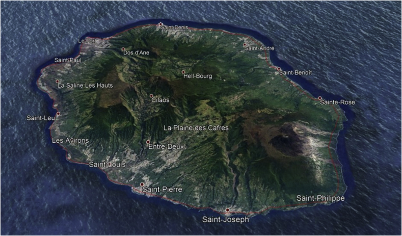
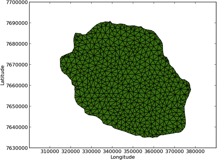
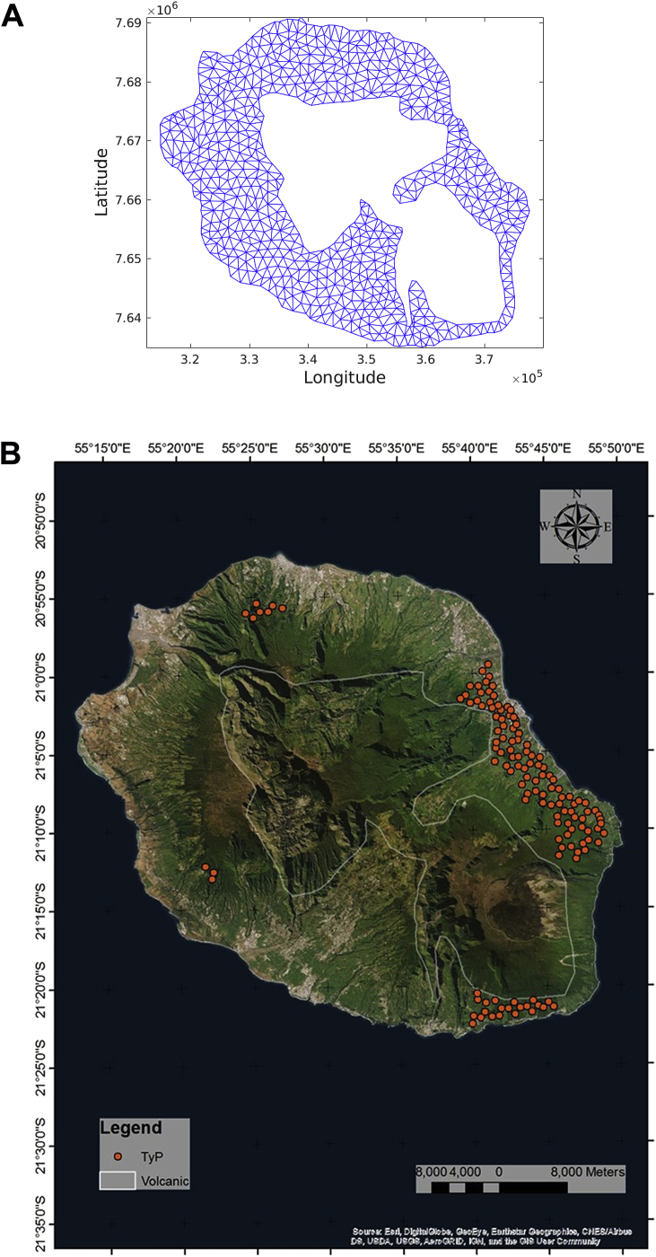
Here we employ the values of $\beta =0.14$ and ${\beta }_v=0.4$ reported by Yakob et al. (Yakob & Clements, 2013), and the quotient $\frac{N}{n_v}$ is obtained from the initial conditions. Table 1 summarizes the parameters and values for the numerical simulations. We consider the Chikungunya outbreak at Reunion Island (population $\approx$ 770,000). Between March 1, 2005, and April 30, 2006, approximately 255,000 cases were reported in this French territory in the Indian Ocean, Renault et al. (Renault et al., 2007). Fig. 1 shows the domain obtained by using a geographical information system and a generated unstructured triangular mesh in utm units.

Table 1.

Parameters of the Chikungunya spread model.

Parameter	Value	Description
β	0.14	mosquito to human transmission
${\beta }_v$	0.4	human to mosquito transmission
k	0.5	reciprocal of host latent period
η	0.5	reciprocal of mosquito latent period
γ	0.25	host recovery rate per day
μ	0.05	reciprocal of mosquito life span in days

Fig. 1.

Area of study.

3.1. Mobility

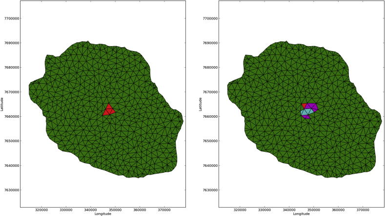
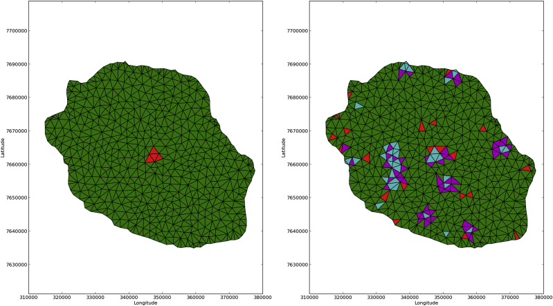
Human mobility, especially the infected individuals, can create multiple disease waves resulting in substantial deviation from mean field results. In general, human mobility makes the infection spread faster and eventually produces an apparent early suppression due to secondary waves creating recovered regions which block the spread of the primary epidemic wave. Fig. 2, Fig. 3 show 20 days spatial spread simulations, no host mobility and host mobility ($p_{mob}=0.5$, $\lambda =0.5$ ) respectively. Here susceptible cells are colored in green, exposed in magenta, infectious in red and recovered in cyan; initially 765,000 humans were homogeneously distributed (same number per cell) with $m=5$ vectors per host (literature reports uses of m in the range $1\le m\le 10$) and closed boundary conditions. An initial seed of 4 infected humans were located at 4 central cells. In the simulation that includes mobility, we can appreciate secondary epicenters at large distances from the original seed as a direct consequence of the mobility effects. Numerical results reported by Santos et al. (Santos et al., 2009) agree with this observation.

Fig. 2.

20 days simulation no host mobility, an infection wave moving outward.

Fig. 3.

20 days simulation host mobility $p_{mob}=0.5$, $\lambda =0.5$.

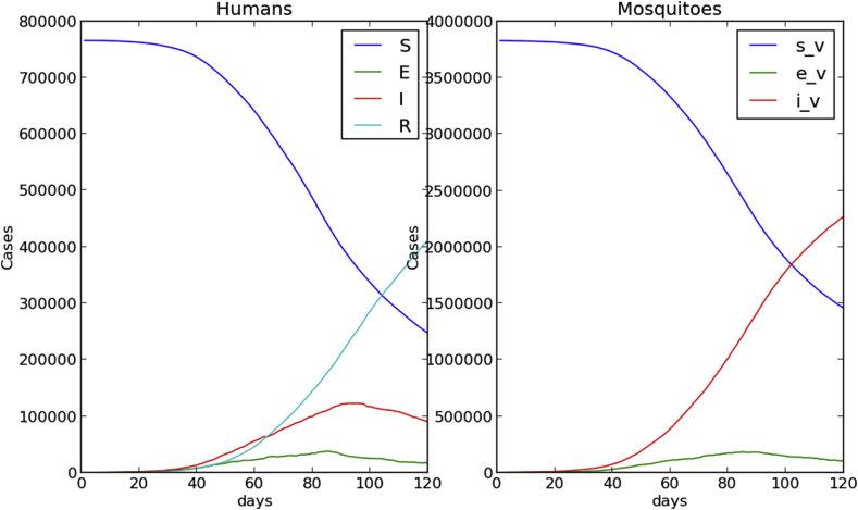
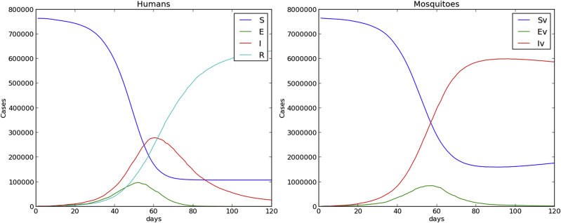
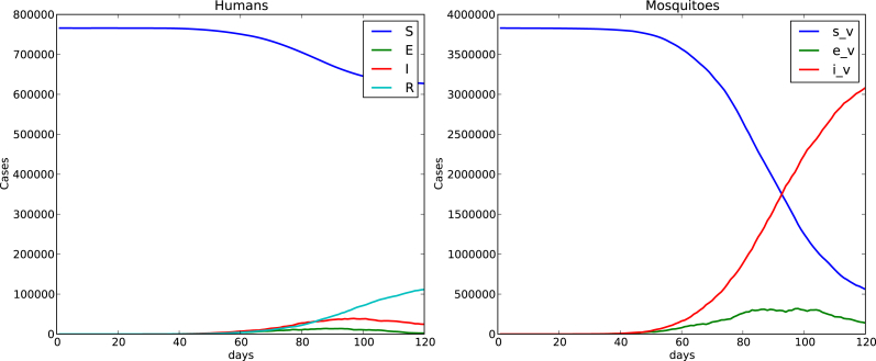
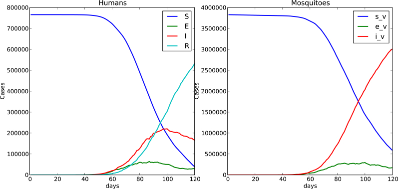
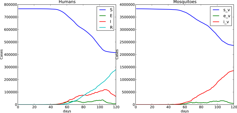
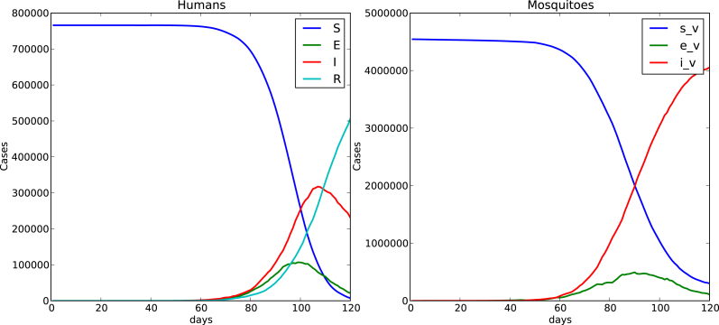
Fig. 4, Fig. 5 show time evolution of the diseases among human and mosquito populations. A remarkable difference in the peak size and duration of the number of infected humans (an early suppression of the disease) is observed when we compare simulations with mobility and no mobility of humans.

Fig. 4.

120 days simulation no host mobility.

Fig. 5.

120 days simulation host mobility $p_{mob}=0.5$, $\lambda =0.5$.

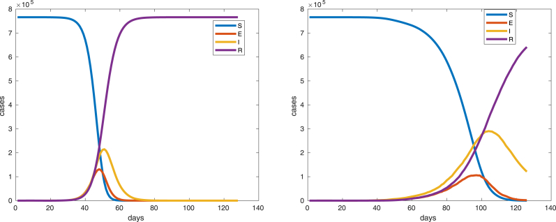
Fig. 6 shows a comparison of the time evolution of the infection among humans between the ode model and the cellular automata model where mosquitos and humans are assumed homogeneously distributed over the whole domain.

Fig. 6.

Left ode model, right cellular automata model simulation,I(0) = 1, $m=5$ mosquitos per human, 766000 total human population, human mobility probability $p_{mob}=0.5$, $\lambda =0.5$.

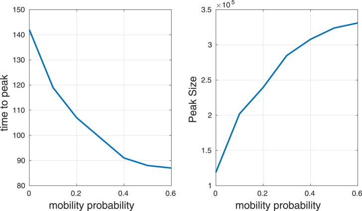
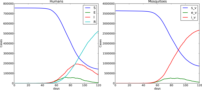
Fig. 7 shows the time to get the peak and the peak (maximum number of infected humans) as function of the mobility probability. Mobility increases the peak and decreases the time to get it. This suggests that mobility makes the infection spread faster and eventually produces an apparent early suppression, which agrees with the numerical results observed by de Castro et al. (De Castro Medeiros et al., 2011), Enduri and Jolad (Enduri & Jolad, 2014). Here a 120 days simulation was run with homogeneous distribution of host and vectors (the main outbreak of Chikungunya for Reunion Island occurred over a period of 18 weeks thus we assumed a 120 days as a simulation time), 5 vectors per human and an initial seed of 4 infected humans was located at a mosquito populated cell.

Fig. 7.

Time to get the peak and peak size as a function of mobility probability $p_{mob}$.

3.2. Heterogeneity

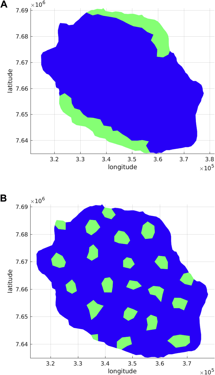
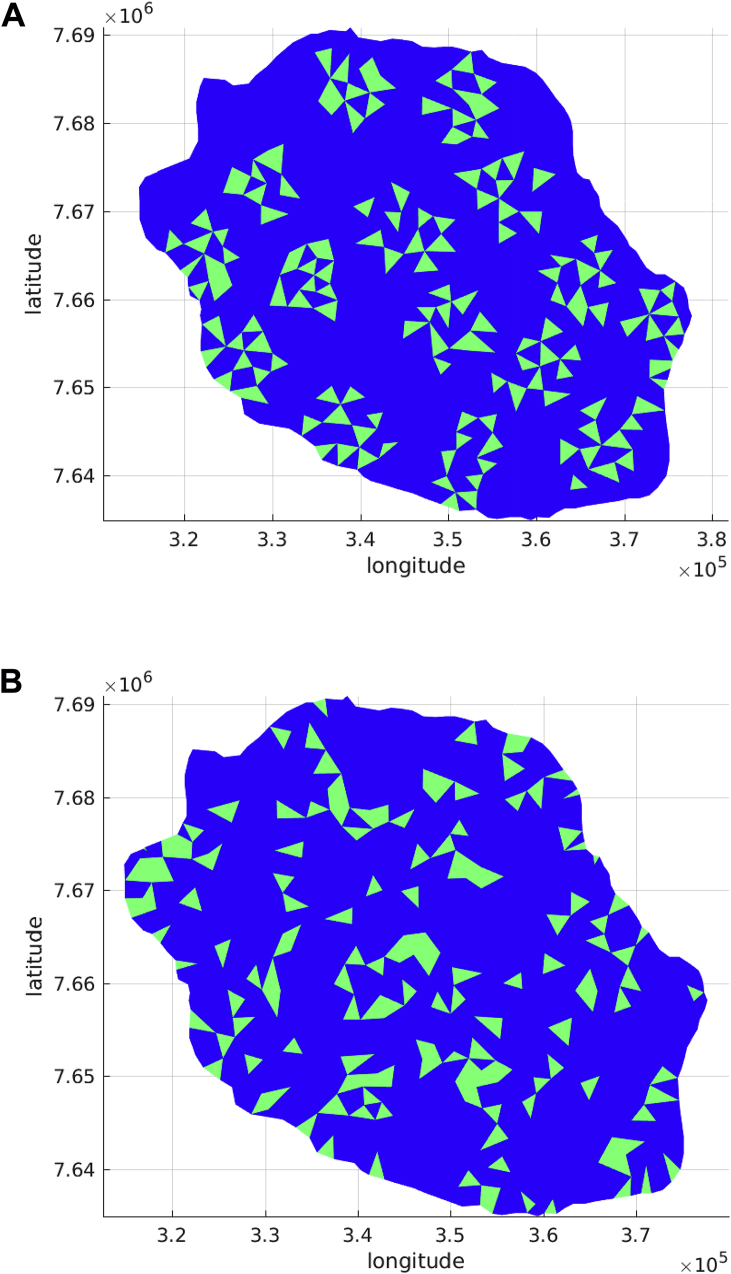
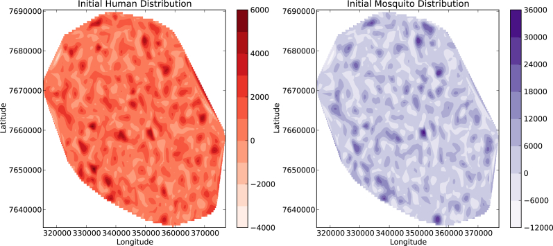
The heterogeneity of mosquito bites to humans during the spread of Chikungunya virus is an important factor that should be considered when modeling the dynamics of mosquito borne diseases spread. Traditional models generally assume homogeneous mixing between humans and vectors, which is not quite consistent with reality. Uneven distribution of blood-meal hosts and larval habitat creates a spatial mosaic of demographic sources and sinks. In addition, mosquito populations fluctuate temporally, forced by weather variables such as rainfall, temperature and humidity. These sources of spatial and temporal heterogeneity in the distribution of mosquito populations generate variability in the human biting rate, the proportion of mosquitos that are infectious and in the risk of human infection. It is clear that in order to run a simulation, an initial seed of infection either of humans or mosquitos must be assumed, but it is also important to state the initial spatial distribution of hosts and vectors. This can be achieved in different ways, assuming constant average number of either host or vectors in the whole domain or in a reduced number of localized cells. The reduced number of localized cells can be fill with either host or humans using evenly (same number of hosts and vectors per cell), randomly uniform or Poisson distributed. Setting appropriate initial conditions is relevant because spatially heterogeneous transmission may arise due to spatial variation in vector habitat and human population density.To show the influence of the initial population distributions, we defined four space initial distributions: two patches, several patches, random clustered patches and random patches. All these spatial distributions are assumed to be composed by 150 cells which is approximately a 15% coverage of the total number of cells. Fig. 8, Fig. 9 present these domains.

Fig. 8.

Initial distributions Patches.

Fig. 9.

Initial Conditions randomly distributed.

For the following numerical simulations we consider different ways to distribute host and vectors on the two patches spatial distribution, these are labelled by cases 1 to 5. The human population is assumed 766000 with 5 mosquitos per human, an initial condition of $I\left(0\right)=4$ in a mosquito populated cell is taken and the human mobility probability is $p_{mob}=0.5$ with $\lambda =0.5$.

Case 1

We start by assuming humans localized in these cells and mosquitos evenly distributed in the whole domain, as in the case of homogeneous distribution (the main assumption of the ode model) a human population of 766000 and 5 mosquitos per human are considered. A probability of 0.5 for humans mobility produced a high peak for the homogeneous case, however no epidemic occurs for this spatial distribution. This show us that not only is the human mobility important but also the initial spatial distribution of hosts and vectors. Caraco et al. (Caracoa, Duryea, Glavanakov, Maniatty, & Szymanski, 2001) noticed that clumping (clustering) can increase the chance that the pathogen and vector become physically separated during the initial phase of the epidemic process. Spatial aggregation of hosts can increase the fraction of vector attacks directed to already infested hosts. Clumping also generates gaps in the host population which slow down the global advance of the diseases, and the requirement for clump-to-clump dispersal can inhibit diffusive spread of the vector.

Substituting equations (1), (2) in (4) provides

$${\mathcal{R}}_0=\sqrt{a^2{p}_{hv}{p}_{hv}\frac{n_v}{N}\frac{\eta }{\mu \gamma \left(\mu +\eta \right)}}\text{,}$$ (6)

a relation between the basic reproduction number and $m=\frac{n_v}{N}$ the ratio of the number of mosquitos to the number of humans. In the homogeneous case this ratio is assumed constant over the whole domain, in the particular case of humans evenly distributed over a reduced number of localized cells and mosquitos evenly distributed over the whole domain, the clustering of humans makes this ratio

$$\begin{array}{l}m=\frac{\text{number of mosquitos per cell}}{\text{number of humans per cell}}=\frac{\frac{nmph\ast Pob}{TNC}}{\frac{Pob}{RNLC}}\\ =nmph\frac{RNLC}{TNC}\end{array}$$

to be reduced, making the number of no human-populated cells an important factor for spatial spread, here $nmph$ is the original number of mosquitos per human and it is assumed to be equal to 5 at the homogeneous case, $TNC$ and $RNLC$ stand for total number of cells and reduced number of localized cells respectively. In order to start an outbreak for this particular spatial human clustered distribution, $nmph$ was increased up to the value of 85.

Case 2

We assume that mosquitos are clustered over the reduced number of localized cells and humans are evenly distributed over the whole domain. In this case we notice that in the vast majority of cells $m=0$ (no mosquitos), while at mosquito populated cells m has increased,

$$\begin{array}{l}m=\frac{\text{number of mosquitos per cell}}{\text{number of humans per cell}}=\frac{\frac{nmph\ast Pob}{RNLC}}{\frac{Pob}{TNC}}\\ =nmph\ast \frac{\text{total number of cells}}{\text{reduced number of localized cells}}\\ =nmph\ast \frac{\text{TNC}}{\text{RNLC}}\end{array}$$

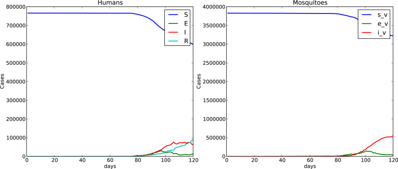
Fig. 10 shows the time spread of the disease for a 120 days simulation with this initial condition. A remarkable difference shows up when we compare this case of localized mosquitos and evenly distributed hosts over the whole domain with the case of humans and vectors homogeneously distributed over the whole domain shown in Fig. 5. Peak is reduced when mosquitos are localized. This reduction in prevalence due to vector clustering was also observed in the numerical simulations performed by Dias and Monteiro (Dias & Monteiro, 2018). The fact that mosquitos are concentrated in a localized area and humans are evenly distributed in the whole domain makes the contacts reduced due to the existence of non mosquito populated areas, reducing the number of bitten humans (exposed) and the number of infected humans. The number of infected mosquitos was also reduced.

Case 3

Here we assume an initial condition with both humans and mosquitos evenly distributed over the reduced number of cells. In comparison with Fig. 10 where humans were evenly distributed over the whole domain and mosquitos were clustered over a reduced number of localized cells, we observe that the peak of the number of infected humans is increased, clustering back both mosquitos and humans in the localized area increases the contacts, increases the number of bitten humans (exposed) and the number of infected humans. But we also notice that the number of infected humans in this case is lower (peak reduces and time to peak increases) that the case of humans and mosquitos evenly distributed over the whole domain shown at Fig. 5. Inside each patch the disease is mainly spread by local contacts inside the neighborhoods while the disease moves from patch to patch by means of the human mobility. The mobility probability assumed for humans cause them to move into non mosquito populated areas where humans will not be bitten, thus the disease will not spread in these areas. In Fig. 11 we show the time spread of the disease for this case of mosquitos and human localized over a reduced number of cells. At each localized cell we have

$$m=\frac{\text{number of mosquitos per cell}}{\text{number of humans per cell}}=\frac{\frac{nmph\ast Pob}{RNLC}}{\frac{Pob}{RNLC}}=nmph$$

Case 4

We consider again localized both humans and mosquitos over a reduced number of cells, this time while the humans are evenly distributed, the mosquitos are assumed to be Poisson distributed over the reduced number of cells (Galton board implementation). All the cells have the same amount of humans but some cells are highly, while some others are poorly populated with mosquitos. This reduces the number of infected people and the number of infected mosquitos. Even though more mosquitos are infected in high mosquito populated cells after biting an infected human, few humans in the cell will receive more infectious bites of competing infectious mosquitos.

Case 5

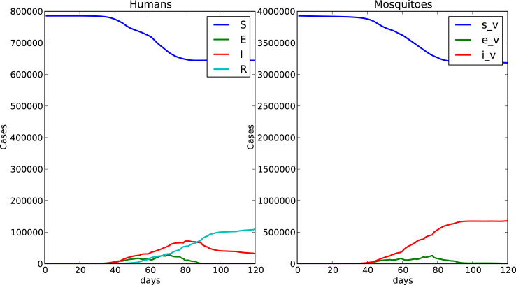
We consider localized humans and mosquitos over a reduced number of cells, with both humans and vectors Poisson distributed, Fig. 13 shows the time evolution of host and vectors. As compared with Fig. 12, the number of infected humans and the number of infected mosquitos decreases due to the clustering of hosts and vectors. With both mosquitos and humans localized and clustered by a Poisson distribution, cells where the rate m is high more humans are bitten by mosquitos but fewer mosquitos get infected due to the competing biting, when infected humans move to low m rate cells the disease transmission decreases, this uneven biting rate due to m produces heterogeneity in the transmission intensity.

Fig. 10.

Humans evenly distributed over the whole domain, localized mosquitos evenly distributed over two patches $p_{mob}=0.5$.

Fig. 11.

Localized human and mosquitos evenly distributed over a reduced number of cells $p_{mob}=0.5$.

Fig. 13.

Localized humans and mosquitos, both Poisson distributed $p_{mob}=0.5$.

Fig. 12.

Localized humans and mosquitos, humans evenly and mosquitos Poisson distributed $p_{mob}=0.5$ over a reduced number of cells grouped as two patches.

Oftentimes a coefficient of variation CV of the ratio of mosquitos to humans is used in landscape ecology to characterize heterogeneity.

$$CV=\frac{s_m}{\bar{m}}$$

here $\bar{m}$ is the average ratio of mosquitos to humans and $s_m$ is the standard deviation associated to this value. Notice that m only makes sense on human populated cells. For the case of homogeneous distributions of both host and vectors over the whole domain, $CV=0$. For Case 1 of localized humans over a reduced number of cells and mosquitos evenly distributed over the whole domain, all the localized cells have the same ratio

$$m=nmph\frac{\text{RNLC}}{\text{TNC}}$$

thus $CV=0$ . In Case 2 of localized mosquitos over a reduced number of cells and humans evenly distributed over the whole domain, $CV$ can be explicitly calculated. Let us denote $r=nmph$, $N=\text{TNC}$ and $k=\text{RNLC}$

$$m_i=\frac{rN}{k},i=1,\cdots ,k,\bar{m}=r$$

$$s_m=\sqrt{\frac{{{\sum }^{}}_{i=1}^N{\left(m_i-\bar{m}\right)}^2}{N-1}}=\sqrt{\frac{{{\sum }^{}}_{i=1}^k{\left(r\frac{N}{k}-r\right)}^2+{{\sum }^{}}_{i=k+1}^N{\left(0-r\right)}^2}{N-1}}$$

$$s_m=r\sqrt{\frac{k{\left(\frac{N}{k}-1\right)}^2+N-k}{N-1}},CV=\frac{s_m}{\bar{m}}=\sqrt{\frac{k{\left(\frac{N}{k}-1\right)}^2+N-k}{N-1}}$$

which for $N=1013$, $k=150$ gives $CV=2.39$. For Case 3 (both mosquitos and humans evenly distributed over a reduced number of cells) again the reduced number of localized cells have the same ratio $m=nmph=5$ and $CV=0$. Finally the calculated coefficients of variation for cases 4 and 5 are respectively $CV=1.384$ and $CV=2.39$. A remarkable reduction in peak is observed when the CV is large, this seems to imply that a high CV (associated with high heterogeneity) produces a reduction in the peak (prevalence). This peak reduction was observed by Kong et al. (Kong et al., 2018), they used negative binomial distribution transmission terms in their numerical simulations to model heterogeneity at the population level. Using simulations with a lattice model Caraco et al. (Caracoa et al., 2001) noticed that increasing heterogeneity in host abundance reduces pathogen prevalence. Cissé et al. (Cissé, Yacoubi, & Gourbiére, 2016) also observed this reduction when considering heterogeneity in a landscape composed of cells referred as good or bad habitats. The peak reduction due to high heterogeneity contrasts with the fact that high human mobility increases the peak by reducing the heterogeneity when humans are spread over the entire domain.

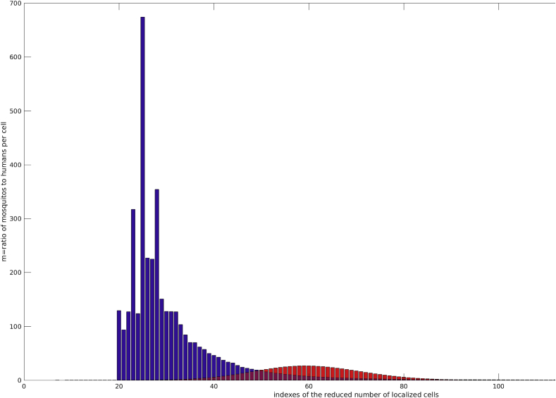
Fig. 14 shows the uneven distribution of m for the cases 4 and 5.

Fig. 14.

Uneven distribution of m over the reduced number of localized cells, Case 4 y red and Case 5 in blue.

This first series of numerical experiments shows the spatial effects of m (the ratio of the number of mosquitos to the number of humans) into the diseases spread. The more unevenly distributed is m (heterogeneous) the smaller the peak and thus diseases prevalence.

Table 2 shows that, to a high heterogeneous spatial distributions corresponds a peak reduction. For Case 3 CV = 0, m is constant over the reduced number of localized cells, here the heterogeneity is due to the fact that in a vast majority of cells $m=0$, this remarks the importance of the number of non mosquito populated areas, thus this type of heterogeneity must be characterized by the mosquito coverage of the domain.

Table 2.

Comparison of contact distributions m.

Case	CV	Normalized peak	time to peak
homogeneous	0	1	92
2	2.39	0.14	88
3	0	0.71	97
4	1.384	0.39	103
5	2.39	0.29	96

Cases 3, 4 and 5 assume that both mosquitos and humans are initially restricted to a reduced number of cells (the whole domain has a vast number of non mosquitos and no human populated cells) but with different spatial distributions over the cells. We define the quantity

$$I_{Nu{m}_{\infty }}=I\left(t_{final}\right)/S\left(0\right)$$

and compute it in order to estimate the persistence. The simulation time was enlarged to 180 days and a human mobility of $p=0.5$ was assumed.

Table 3 shows that besides reducing the peak, heterogeneity due to uneven biting delays the diseases (time to peak increases) and increases persistence. This observation agrees with the theoretical result of Hasibeder and Dye (Hasibeder & Dye, 1988), they established that heterogeneous biting and poor mixing lead to increases in the basic reproduction rates (which measures the persistence of infection), this makes pathogen invasion more likely and elimination more difficult. In their numerical calculations by using a multi-patch analysis Acevedo et al. (Acevedo et al., 2015) also noticed an increase in long-term persistence of infection ($R_0$) due to the spatial heterogeneity in transmission intensity.

Table 3.

Persistence affected by heterogeneity.

Case	CV	Normalized peak	time to peak	$I_{Nu{m}_{\infty }}$
3	0	1	93	0.0174
4	1.384	0.51	115	0.0406
5	2.39	0.34	132	0.0704

Clustering together hosts and vectors evenly distributed over a reduced number of localized cells produced higher peak compared with cases of a reduced number of localized cells with hosts and vectors unevenly distributed. Let us consider this case label as 3 to compare numerical experiments over the different spatial configurations: two patches, multipatches, random clustered and random cells distributed. Fig. 15 show the time evolution of infected, exposed humans and mosquitos for the multipatches configuration. To estimate the fragmentation of these spatial configurations and following Hiebeler (Hiebeler, 2000), we calculate the degree of clustering $q_{00}$ defined as the probability that a random chosen neighboring cell to a vector and host populated cell is also vector and host populated. Table 4 reports the degree of clustering for the spatial configurations.

Fig. 15.

Multipatches domain of a reduced number of localized cells, Case 3.

Table 4.

Peak size affected by domain fragmentation.

Case	CV	Degree of	Normalized	Time
		clustering	peak	to peak
two patches	0	0.853	1	99
multipatches	0	0.685	0.20	120
random	0	0.195	–	–
random clustered	0	0.070	–	–

Comparing the two patches Fig. 11 and the multi patches Fig. 15 configurations we notice that, the more fragmented (lower degree of clustering) the localized patches are, the more the peak is reduced. No outbreak is obtained for the random and clustered random configurations that have very low degree of clustering.

In the context of cellular automata implementations this can be explained because the fragmentation (separation between cells) of localized cells makes the transmission harder to take place using local interactions even though human mobility helps the spread of infectious hosts. Each localized cell has the same number of mosquitos and humans, thus m is constant and $CV=0$. Initially heterogeneity is due to the number of non mosquito and humans populated areas in the two patches spatial configuration, in the subsequent spatial configurations (multipatches, random and clustered random), heterogeneity is increased by the spatial fragmentation (separation) of cells. This suggests that fragmentation of mosquito and human populated areas plays an important roll in the diseases spread that needs to be quantified.

Due to human mobility, some approaches could assume humans and mosquitos randomly distributed over the entire domain. In order to discuss this case we assume a random selection of cells, at each cell the number of humans is randomly selected, $rand\left(\right)\ast area\ast average$ depending on its area and by using the census data for Reunion Island with and average 330 people per square kilometer, the amount of mosquitos is randomly selected $rand\left(\right)\ast \text{number of humans}$ in the range $rand\left(\right)\in \left\{\mathrm{0,1},\dots 10\right\}.$The initial condition generated in this way produces $S\left(0\right)=763750,s_v\left(0\right)=3727546$. An initial seed $I\left(0\right)=1$ is assumed. Fig. 16 shows the time domain evolution of the diseases assuming an initial condition with humans and mosquitos randomly distributed over the entire domain which is quite similar to the case of both humans and mosquitos homogeneously distributed, Fig. 17 shows this distribution where $CV=0.59$ and 58.5% of the cells are human populated. In real life mosquitos are not randomly distributed over the entire domain, in fact breeding sites are very localized regions where the amount of mosquitos changes in time due to weather variables such as temperature and rainfall. This suggests that these areas should be identified and constantly being monitored.

Fig. 16.

Time evolution of the diseases spread with an initial condition of mosquitos and humans randomly distributed over the entire domain.

Fig. 17.

Initial condition with randomly distributed hosts and vectors over the whole domain.

Fig. 18 presents the time evolution of infected humans and mosquitos for a simulation run over a reduced spatial domain. The volcanic area localized at the center of the Reunion Island have been removed from the original domain (we assumed that this area has a very low human population density). For this simulation the initial condition was defined using population data from the Reunion Census 2007 (according to the French Institution for Statistics). Fig. 19 shows on the left the unstructured triangular mesh defined for this modified domain; on the right hand side it shows red points (obtained with a geographical information system) that correspond to cells where annual average temperature resides between 28 and 30 Celsius degrees and annual average precipitation ranges between 250 and 750 mm. We assumed that these points correspond to mosquito breeding sites because they hold appropriate weather conditions for mosquitos reproduction. Five mosquitos per human were assumed, mosquitos were evenly distributed over the breeding sites and an infected human was localized in a mosquito/human populated cell.

Fig. 18.

Time evolution of infected humans and mosquitos, simulation over a reduced computational domain.

Fig. 19.

Modified area of study.

Table 5 shows the information of the two meshes used in the numerical simulations.

Table 5.

Meshes’s information.

Mesh	Nodes	Elements	boundary edges	mean area($m^2$)
Original	581	1013	147	3.95373e+06
Modified	766	1259	273	1.99709e+06

3.3. Vector control measures

Chikungunya virus is spread to people by Aedes aegypti and Aedes albopictus mosquitos. Aedes aegypti is also responsible for the transmission of dengue, zika and Mayaro. These diseases are transmitted as a side-effect of Aedes’ need to obtain blood to complete its life cycle (gravid female mosquitos require blood from a host for their eggs to be viable). Arboviruses, use these mosquitos as vehicles to develop and travel between human hosts. Unfortunately, to date, there exists no effective vaccine to block the transmission of any of these pathogens. Several mosquito-control interventions exist to date and every year more are being developed. Among the traditional Aedes-control interventions, spatial insecticide spraying (also known as fogging) is one of the oldest. Some others include reduction of breeding sites, use of larvicides, reduction of mosquito hosts contacts by: use of bednets or spatial and contact repellents. Recently some of the most promising novel interventions have been: the sterile insect, release of Wolbachia-infected mosquitos and release of insects carrying a dominant lethal gene (RID).To include vector control measures as Moulay et al. (Moulay, Aziz-Alaoui, & Kwon, 2012) proposed, at the cellular automata implementation we assume that locally at each cell some important diseases spread variables are modified:

$$\begin{array}{c}S’=-\beta \left(1-u_4\left(t\right)\right)S\frac{i_v}{n_v}\\ E’=\beta \left(1-u_4\left(t\right)\right)S\frac{i_v}{n_v}-kE\\ I’=kE-\gamma I\\ R’=\gamma I\\ s{’}_v={\mu }_b\left(1-u_1\left(t\right)\right)n_v-{\beta }_v\left(1-u_4\left(t\right)\right)s_v\frac{I}{N}-{\mu }_d\left(1+u_2\left(t\right)\right)s_v\\ e{’}_v={\beta }_v\left(1-u_4\left(t\right)\right)s_v\frac{I}{N}-\eta \left(1+u_3\left(t\right)\right)e_v-{\mu }_d\left(1+u_2\left(t\right)\right)e_v\\ i{’}_v=\eta \left(1+u_3\left(t\right)\right)e_v-{\mu }_d\left(1+u_2\left(t\right)\right)i_v\end{array}$$

Here ${\mu }_b$ is the mosquito birth rate, ${\mu }_d$ is the mosquito death rate. We assume that locally (each cell) these quantities are different. The time dependent function $u_1\left(t\right)$ is a control that reduces the mosquito birth rate, it models vector control measures related to reduction of breeding sites or use of larvicides. Function $u_2\left(t\right)$ is a control that increases the mosquito death rate, it models vector control strategies directed to kill mosquitos for instance fogging or mosquito traps. Function $u_3\left(t\right)$ is a control that increases extrinsic incubation period that we use to simulate wMel Wolbachia effects. Finally $u_4\left(t\right)$ is a control that represents efforts made for prevention over the time simulation interval. It mainly consists in reducing the number of vector-host contacts using repellents against adult mosquitos, protecting with mosquito bednets or wearing appropriate clothing. According to the meteorological analysis for precipitation reported by Boyer et al. (Boyer, Foray, & Dehecq, 2014) and Garot et al. (Garot, Joët, Combes, & Lashermes, 2018), the highest precipitation areas In Reunion Island are on the East coast. We consider vector control measures localized only over the East (right side of the domain that corresponds to 50% coverage of the total domain). The numerical experiments are conducted with the randomly generated initial distribution shown at Fig. 17. We separately consider increasing by four times the mosquito death rate what we call $C_1$ and reducing by four times the mosquito birth rate that we called $C_2$. We also considered control $C_3$ which refers to both control $C_1$ and $C_2$ but applied over the cells that satisfy $m>1$ which conforms 30% of coverage of the entire domain. $C_4$ refers to a control measure over the right hand side domain where the extrinsic incubation period is assumed to be enlarged to 14 days (originally it was assumed a 2 days period) in order to simulate wMel-infected mosquitos when exposed to CHIKV. If we assume all the East region is populated by wolbachia infected mosquitos no outbreak arises, so we relaxes this assumption allowing that only a 50% of mosquito population is infected by Wolbachia. As reported by Aliota et al. (Aliota et al., 2016) Wolbachia infection does not completely ablate transmission of virus, but rather delays the extrinsic incubation period (EIP) of the virus and reduces the transmission potential of CHIKV-infected mosquitos. Finally we called $C_5$ the control that allows to reduce one fourth of the original value of vector-hosts contacts, this simulates the use of repellents, bednets and protective clothing. We use the numerical results to compute the quantity

$$S_{Nu{m}_{\infty }}=\frac{S\left(t_{final}\right)}{N}$$

the portion of humans that escape the outbreak, $t_{final}$ is the final time of the simulation. The greater this quantity is, the better the control measure. Table 6 summarizes the results for these vector control measures. Direct kill of mosquitos seems to be not the best control measure; it greatly improves when combined with the use of larvicides over the East side of the domain approximately 50% coverage. We note that better results can be obtained applying these two controls over a reduced number of non clustered cells (those that satisfy $m>1$, approximately a 30% coverage of the domain) which is a good choice provide this quantity m is being monitored over the study area. For instance, Vanwambeke et al. (Vanwambeke, Bennet, & Kapan, 2011) use land cover and land use data to produce high resolution vector-to-host ratio maps to estimate risk of exposure. Excellent results (not outbreak) are obtained if all the mosquitos are assumed Wolbachia infected and even in the case that only 50% of the mosquitos are Wolbachia infected, good results are acquired. For this vector control measure we assumed that the amount of wolbachia infected mosquitos was not time-space dependent. Some further improvements of our implementation can include the time-space dispersal of wolbachia infected mosquitos as Schmidt et al. (Schmidt et al., 2017) proposed it. It drags our attention the good performance of the control related to reducing the number of vector-hosts contacts by using repellents, bednets or protective clothing. We simulated it over the right hand side of the domain but it can be broadly implemented over the whole domain. We believe that, public health agencies should encourage this type of measure by providing free or low cost repellents, bednets or protective clothing and implementing public media campaigns to reduce the mosquito host contact rates.

Table 6.

Comparison of vector control measures.

Type	Time to peak	Normalized peak	$S_{Nu{m}_{\infty }}$
No control	86	1	0.1052
$C_1$	97	0.91	0.1812
$C_2$	97	0.96	0.1421
$C_1$ & $C_2$	98	0.83	0.2118
$C_3$	103	0.83	0.2185
$C_4$	105	0.95	0.1785
$C_5$	106	0.90	0.2136

3.4. Seasonality

As with any other vector-borne diseases, Chikungunya disease transmission involves host, vector and pathogen and it is greatly influenced by weather factors such as temperature and rainfall. Rainfall creates breeding habitats for vectors and temperature has a major role for both mosquitos, virus development and transmission. Parameters such as vector-human transmission rate, human-vector transmission rate, extrinsic incubation, birth and mortality vector rates are sensitive to temperature and hence, $R_0$ is also highly sensitive to climate. Zhu et al. (Zhu et al., 2019) and Kakarla et al. (Kakarla et al., 2019) reported relations for the extrinsic incubation rate, mortality mosquitos rate, human-vector, vector-human transmission probabilities as functions of temperature

$$\eta \left(T\right)=\frac{1}{4+e^{5.15-0.123T}}$$

$$\mu \left(T\right)=0.8692-0.159T+0.01116T^2-3.408\times {10}^{-4}{T}^3+3.809\times {10}^{-6}{T}^4$$

$$p_{hv}\left(T\right)=\{\begin{array}{ll}0\hfill & T<12.4\hfill \\ 0.0729T-0.9037\hfill & 12.4\le T\le 26.1\hfill \\ 1\hfill & T>26.1\hfill \end{array}$$

$$p_{vh}\left(T\right)=\{\begin{array}{ll}1.044\times {10}^{-3}T\left(T-12.286\right)\sqrt{32.461-T}\hfill & 12.286\le T\le 32.461\hfill \\ 0\hfill & \text{otherwise}\hfill \end{array}$$

where T is the ambient temperature in Celsius.

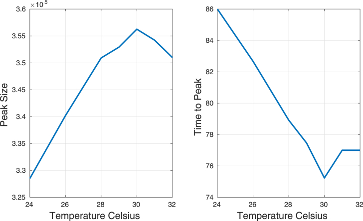
Assuming a constant temperature over the whole domain, a 120 days simulation was run. We observed that the number of infected humans has a maximum peak at temperature ${30}^0$C. When temperature increases the time to peak is reduced until reach ${30}^0$C, then it starts to increase. Fig. 20 shows the variation of disease peak (prevalence) and time to reach the peak as a functions of temperature. Constant (in space and time) temperatures were assumed.

Fig. 20.

Peak and time to peak as functions of temperature.

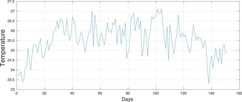
Now, let us consider a time series for the temperature, data were obtained from the METEOR meteorological data repository (https://smartis.re/METEOR) and averaged over the entire domain. This five months data series has a mean of 25.55, variance 0.6718, with 23.3 and 27.1 as minimum and maximum temperatures respectively. Fig. 21 shows the time series for the temperature. Using this series and just by adding the constant values [-4,-3,-2,-1,0,1,2,3,4] we generated another eight time series, basically we have the original time series with a translation in the mean.

Fig. 21.

Time series for the temperature.

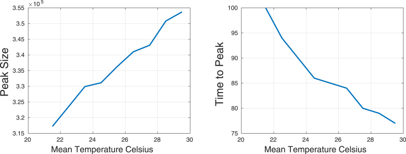
Fig. 22 shows the effects of the mean temperature over the peak of the number of infected humans and the time to reach this peak. As mean temperature increases we observed an increase in the peak of the number of infected humans and a reduction in the time to reach this peak. Huber et al. (Huber, Childs, Caldwell, & Mordecai, 2018) also observed that at both constant and seasonality varying temperatures, warmer temperatures at the start of the epidemics promote more rapid epidemics due to faster burnout of the susceptible population.

Fig. 22.

Peak Size and time to peak as functions of the mean temperature.

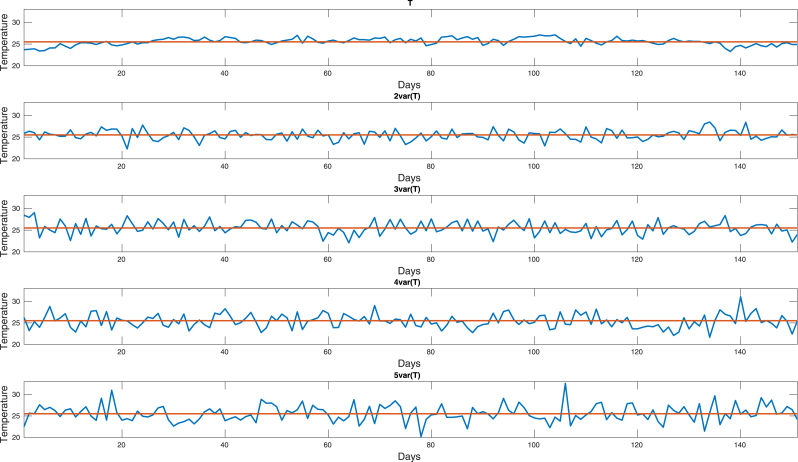
In order to examine the effects of temperature fluctuations in the peak size and time to peak, we use the mean $mean\left(T\right)$ and variance $var\left(T\right)$ of the temperature time series (weather data from Meteor) to generate another four times series with the same mean and approximately $k\ast var\left(T\right),k=\mathrm{2,3,4,5}$ variances. Fig. 23 shows these series where variance increases from the top to the bottom.

Fig. 23.

Generated time series for the temperature.

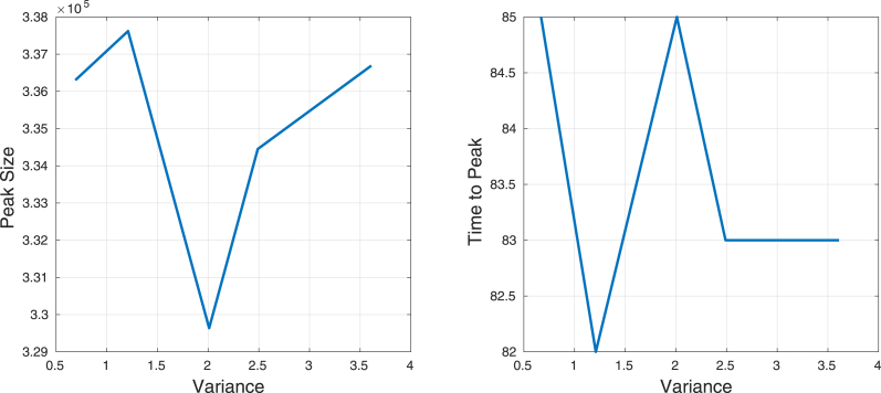
Fig. 24 shows the effects of the fluctuation in the temperature (variance) over the peak of the number of infected humans and the time to reach this peak. It seems that when variance increases, both peak and time to reach the peak oscillate.

Fig. 24.

Peak size and time to peak as functions of the fluctuations in temperature.

3.5. Discussion

Cellular automata formulations allow us to consider local interactions of infected due to neighboring cells and global interactions due to human mobility probability. The probability that a susceptible host (vector) acquires the pathogen depends on the local density of infectious vectors (hosts), rather than their global density. The numerical experiments showed the importance of the spatial distribution of hosts and vectors, locally the ratio m of mosquitos to humans produces local reproduction numbers. Two types of heterogeneities are identified, those due to the uneven bitting (different values of m at each cell) and spatial heterogeneities (sinks) due to fragmentation. Increasing the human mobility reduces the initial heterogeneity, it asymptotically increases the peak and reduces the time to the peak. Besides reducing the peak (prevalence), heterogeneity due to uneven biting delays the diseases (time to peak increases) and increases its persistence. At each cell, control vector strategies are implemented by assuming increments in the extrinsic incubation period and mosquito death rates, or reduction of host/vector contact rates and mosquito birth rate. All these quantities are assumed to be time and space dependent. Space heterogeneities are accounted locally by using population densities for human and mosquitos; seasonality is easily implemented by assuming that extrinsic incubation rates, mosquito’s birth rate and vector-human/human-vector transmission probabilities are functions of temperature (time-space dependent). All these features make cellular automata and attractive method to perform mosquito-borne diseases simulations.

4. Conclusions

We have proposed the use of a cellular automata defined on an unstructured triangular grid to model and simulate the Chikungunya spread. The cellular automata was obtained from a $SEIR\_sei$ ode model for chikungunya diseases spread. Transmission probabilities from human to vector and vector to human were globally defined using a relation between the transmission rates and the ratio of mosquitos to humans, locally the probabilities were modified by the number of infected humans and mosquitos inside the neighborhood. The numerical experiments showed that human mobility increases the peak size of the number of infected humans and reduces the time to reach this peak. Heterogeneity due to uneven biting reduces the peak, delays the diseases and increases the diseases persistence. Increases in the mean temperature produce an increase in peak and reduction in time to peak, on the other hand increasing the variance seems to make this quantities to oscillate. The easy implementation of this model has some advantages that allow some future extensions. For instance, models that include more compartments such as mosquito dynamics stages: egg, larvae, puppa. Dengue models with four strains or coinfection models as simultaneous outbreaks of dengue, chikungunya and Zika virus. If required, at some spatial scales mosquito movements can be included in the cellular automata model, locally at each neighborhood mosquitos can be assumed to move to the most human populated cell (mosquitos tend to cluster near humans).

Handling Editor: Dr. J Wu

References

- Acevedo M., Prosper O., Lopiano K., Ruktanonchai N., Caughlin T., Martcheva M. Spatial heterogeneity, host movement and mosquito borne disease transmission. PLoS One. 2015;10(6) doi: 10.1371/journal.pone.0127552. [DOI] [PMC free article] [PubMed] [Google Scholar]
- Aliota M.T., Emma C.W., Yepes A.U., Velez I.D., Christensen B.M., Osorio J.E. The wMel strain of wolbachia reduces transmission of chikungunya virus in Aedes aegypti. PLoS Neglected Tropical Diseases. 2016;10(4) doi: 10.1371/journal.pntd.0004677. [DOI] [PMC free article] [PubMed] [Google Scholar]
- Batty M. MIT Press; 2005. Cities and complexity: Understanding cities with cellular automata, agent-based models, and fractals. [Google Scholar]
- Boyer S., Foray C., Dehecq J.S. Spatial and temporal heterogeneities of Aedes albopictus density in the Reunion Island: Rise and weakness of entomological indices. PLoS One. 2014;9(3) doi: 10.1371/journal.pone.0091170. [DOI] [PMC free article] [PubMed] [Google Scholar]
- Brauer F., Castillo-Chavez C., Mubayi A., Towers S. Some models for epidemics of vector-transmitted diseases. Infectious Disease Modelling. 2016;1(1):79–87. doi: 10.1016/j.idm.2016.08.001. [DOI] [PMC free article] [PubMed] [Google Scholar]
- Caracoa M., Duryea M., Glavanakov S., Maniatty W., Szymanski B. Host spatial heterogeneity and the spread of vector-borne infection. Theoretical Population Biology. 2001;59(3):185–206. doi: 10.1006/tpbi.2000.1517. [DOI] [PubMed] [Google Scholar]
- Cissé B., Yacoubi S., Gourbiére S. The spatial reproduction number in a cellular automaton model for vector-borne diseases applied to the transmission of Chagas disease. Simulation, Special Issue: Simulation with Cellular Automata. 2016;92(2) [Google Scholar]
- De Castro Medeiros L.C., Castilho C.A., Braga C., De Souza W.V., Regis L., Monteiro A.M. Modeling the dynamic transmission of dengue fever: Investigating disease persistence. PLoS Neglected Tropical Diseases. 2011;5(1):e942. doi: 10.1371/journal.pntd.0000942. [DOI] [PMC free article] [PubMed] [Google Scholar]
- Deutsch A., Dormann S. 2005. Cellular automaton modeling of biological pattern formation, Birkhäuser Boston. [Google Scholar]
- Dias J., Monteiro L. Clustered breeding sites: Shelters for vector-borne diseases. Computational and Mathematical methods in Medicine. 2018:2575017. doi: 10.1155/2018/2575017. [DOI] [PMC free article] [PubMed] [Google Scholar]
- Enduri M.K., Jolad S. Dynamics of Dengue with human and vector mobility. Spatial and Spatio-temporal Epidemiology. 2014;25:57–66. doi: 10.1016/j.sste.2018.03.001. [DOI] [PubMed] [Google Scholar]
- Garot E., Joët T., Combes M.C., Lashermes P. Vol. 122. Springer Nature; Heredity: 2018. pp. 833–847. (Genetic diversity and population divergences of an indigenous tree (Coffea mauritiana) in Reunion Island: Role of climatic and geographical factors, the genetic society). 6. [DOI] [PMC free article] [PubMed] [Google Scholar]
- Hasibeder G., Dye C. Population dynamics of mosquito-borne disease: Persistence in a completely heterogeneous environment. Theoretical Population Biology. 1988;33:31–53. doi: 10.1016/0040-5809(88)90003-2. [DOI] [PubMed] [Google Scholar]
- Hiebeler D. Populations on fragmented landscapes with spatially structured heterogeneities: Landscape generation and local dispersal. Ecology. 2000;81(6):1629–1641. doi: 10.1007/s00285-006-0054-6. [DOI] [PubMed] [Google Scholar]
- https://smartis.re/METEOR.
- Huber J., Childs M., Caldwell J., Mordecai Seasonal temperature variation influences climate suitability for dengue, chikungunya and dengue transmission. Neglected Tropical Diseases. 2018;12:5. doi: 10.1371/journal.pntd.0006451. [DOI] [PMC free article] [PubMed] [Google Scholar]
- Kakarla S.G., Mopuri R.1, Mutheneni S.R., Bhimala K.R., Kumaraswamy S., Kadiri M.R. Temperature dependent transmission potential model for chikungunya in India. The Science of the Total Environment. 2019;647:66–74. doi: 10.1016/j.scitotenv.2018.07.461. [DOI] [PubMed] [Google Scholar]
- Kong L., Wang J., Li Z., Lai S., Liu Q., Wu H. Modeling the heterogeneity of dengue transmission in a city. International Journal of Environmental Research and Public Health. 2018;15:6. doi: 10.3390/ijerph15061128. [DOI] [PMC free article] [PubMed] [Google Scholar]
- Moulay D., Aziz-Alaoui M.A., Kwon H.D. Optimal control of chikungunya disease: Larvae reduction, treatment and prevention. Mathematical Biosciences and Engineering. 2012;9(2):369–392. doi: 10.3934/mbe.2012.9.369. [DOI] [PubMed] [Google Scholar]
- Ortigoza G. Unstructured triangular cellular automata for modeling geographic spread. Applied Mathematics and Computation. 2015;258:520–536. [Google Scholar]
- Ortigoza G., Brauer F., Lorandi A. Mosquito-borne diseases simulated by cellular automata: A review. International Journal of Mosquito Research. 2019;6(6):31–38. http://www.dipterajournal.com/pdf/2019/vol6issue6/PartA/6-5-15-197.pdf In press. [Google Scholar]
- Ortigoza G., Lorandi A., Brauer F. Modelación matemática de la propagación del Chikungunya: Logros y retos. Revista de Investigación en Ciencias de la Salud de la universidad veracruzana. 2019;4(1):6–15. [Google Scholar]
- Renault P., Solet J.L., Sissoko D., Balleydier E., Larrieu S. A major epidemic of chikungunya virus infection on Réunion island, France, 2005-2006. The American Journal of Tropical Medicine and Hygiene. 2007;77:727–731. [PubMed] [Google Scholar]
- Santos L.B.L., Costa M.C., Pinho S.T.R., Andrade R.F.S., Barreto F.R., Teixeira M.G. Periodic forcing in a three-level cellular automata model for a vector-transmitted disease. Physical Review E. 2009;80:1. doi: 10.1103/PhysRevE.80.016102. [DOI] [PubMed] [Google Scholar]
- Schmidt T.L., Barton N., Rasic R., Turley A., Montgomery B., Iturbe I. Local introduction and heterogeneous spatial spread of dengue-suppresing wolbachia through and urban population of Aedes aegypti. PLoS Biology. 2017 doi: 10.1371/journal.pbio.2001894. 15-5. [DOI] [PMC free article] [PubMed] [Google Scholar]
- Sloot P., Hoekstra A.G. Springer Berlin Heidelberg; 2001. Cellular automata as a mesoscopic approach to model and simulate complex systems. [Google Scholar]
- Vanwambeke S., Bennet S., Kapan D. Spatially disggregated disease transmission risk: Land cover, land use and risk of dengue transmission on the island of Oahu. Tropical Medicine and International Health. 2011;16(2):174–185. doi: 10.1111/j.1365-3156.2010.02671.x. [DOI] [PMC free article] [PubMed] [Google Scholar]
- Yakob L., Clements A. A mathematical model of chikungunya dynamics and control: The major epidemic on Réunion island. PLoS One. 2013;8(3) doi: 10.1371/journal.pone.0057448. [DOI] [PMC free article] [PubMed] [Google Scholar]
- Zhu G., Liu T., Xiao J., Zhang B., Song T., Zhang Y. Effects of human mobility, temperature and mosquito control on the spatiotemporal transmission of dengue. The Science of the Total Environment. 2019;651(1):969–978. doi: 10.1016/j.scitotenv.2018.09.182. [DOI] [PubMed] [Google Scholar]