Bayesian inference for dynamical systems

Abstract

Bayesian inference is a common method for conducting parameter estimation for dynamical systems. Despite the prevalent use of Bayesian inference for performing parameter estimation for dynamical systems, there is a need for a formalized and detailed methodology. This paper presents a comprehensive methodology for dynamical system parameter estimation using Bayesian inference and it covers utilizing different distributions, Markov Chain Monte Carlo (MCMC) sampling, obtaining credible intervals for parameters, and prediction intervals for solutions. A logistic growth example is given to illustrate the methodology.

1. Introduction

A common method for performing parameter estimation for dynamical systems is to use Bayesian inference (Ghasemi et al., 2011; Higham & Husmeier, 2013; Ma & Berndsen, 2014; Periwal et al., 2008; Vanlier, Tiemann, Hilbers, & van Riel, 2012). Despite the popularity of using Bayesian inference for performing parameter estimation for dynamical systems and useful computational manuals, there is a need for a formalized and comprehensive methodology.

The methods described in this paper assume that the behaviors of the dynamical system of interest have been mathematically analyzed and that the solutions of the dynamical system are well-behaved. Additionally, it is assumed that if a numerical scheme is being used to solve the dynamical system that the numerical scheme is stable. The methodology is presented from a mathematical biology perspective and it will focus on systems of ordinary differential equations (ODEs); however, the Bayesian inference methodology presented can be applied to other areas of applied mathematics and other differential equations systems such as partial differential equations (PDEs). This paper will provide a formalized methodology for dynamical system parameter estimation using Bayesian inference and it will cover utilizing different distributions, Markov Chain Monte Carlo (MCMC) sampling, obtaining credible intervals for parameters, and prediction intervals for solutions. The methodology is illustrated by using a logistic growth example.

2. Dynamical system

Assume that the dynamical system of interest can be described by the following autonomous ODE system (1) written as a vector differential equation:

$$\mathbf{x}’=\mathbf{f}\left(\mathbf{x}\right),$$ (1)

where $\mathbf{x}=⟨x_1,\dots ,x_k⟩$ and $\mathbf{f}=⟨f_1\left(\mathbf{x}\right),\dots ,f_k\left(\mathbf{x}\right)⟩$, with the vector of initial conditions ${\mathbf{x}}_0=⟨x_1^0,\dots ,x_k^0⟩$.

It is assumed that the that the unique solution vector, $\mathbf{x}\left(t\right)$, of system (1) exists and can be obtained either explicitly or using numerical approximation. If a numerical approximation method is used, it is assumed that the numerical approximation scheme is stable.

All the parameters in system (1) will be denoted by the vector $\mathit{\beta }$. If the initial conditions $x_1^0,\dots ,x_k^0$ will also be estimated, then let the initial conditions $x_1^0,\dots ,x_k^0$ be contained in vector $\mathit{\beta }$ as well.

The dependence of the unique solution vector $\mathbf{x}$ on both time, t, and the vector of parameters, $\mathit{\beta }$, will be emphasized and the unique solution vector will be denoted as $\mathbf{x}\left(\mathit{\beta },t\right)$.

3. Data

Suppose there are m time series data sets. It is important to ensure that the correct ODE model solution or combination of ODE model solutions is fit to the $j^{\text{th}}$ time series data set ($j=1,\dots ,m$).

Sometimes a data set is scaled differently than the model solutions or the data set can be described by a summation of the ODE model solutions. In order to include these situations, we can use a linear combination of the ODE model solutions, $a_1^j{x}_1\left(\mathit{\beta },t\right)+\dots +a_k^j{x}_k\left(\mathit{\beta },t\right)$, to fit to the $j^{\text{th}}$ time series data set. (The simpler case where only the $i^{\text{th}}$ specific ODE model solution $x_i\left(\mathit{\beta },t\right)$ is to be fit to the $j^{\text{th}}$ time series data set, is included in the linear combination where $a_i^j=1$ and the other constants are zero.) If the nonzero vector of constants, ${\mathbf{a}}^j$, will be estimated, then let the nonzero vector of constants, ${\mathbf{a}}^j$, for $j=1,\dots m$, be contained in vector

$$\mathit{\nu }=\left[\begin{array}{c}\mathit{\beta }\\ {\mathbf{a}}^1\\ ⋮\\ {\mathbf{a}}^m\end{array}\right].$$

Also, if the $j^{\text{th}}$ data set can be described by a nonlinear combination of the ODE model solutions, then, similarly, let any estimated nonzero vector of constants, ${\mathbf{a}}^j$, be contained in vector

$$\mathit{\nu }=\left[\begin{array}{c}\mathit{\beta }\\ {\mathbf{a}}^1\\ ⋮\\ {\mathbf{a}}^m\end{array}\right].$$

So, in general, we fit the function, $F\left(x_1\left(\mathit{\beta },t_i^j\right),\dots ,x_k\left(\mathit{\beta },t_i^j\right),{\mathbf{a}}^1,\dots ,{\mathbf{a}}^m\right)$, to the $j^{\text{th}}$ data set.

4. Distribution of data over time

The distribution of the observations over time for each $j^{\text{th}}$ data set must be chosen before fitting system (1) to the data. The following sections will describe the Gaussian, Poisson, Negative Binomial, and other distribution options.

4.1. Gaussian distribution

Let Y be a random variable from the Gaussian distribution with parameters μ and ${\sigma }^2=\frac{1}{\tau }>0$, $Y~\text{N}\left(\mu ,{\theta }^2\right)$. The formulation of the Gaussian distribution is given by the following continuous probability density function (pdf), $f\left(y\right)$ (Bain & Engelhardt, 1987):

$$f\left(y\right)=\frac{1}{\sqrt{2\pi {\sigma }^2}}\text{exp}\left(-\frac{1}{2{\sigma }^2}{\left(y-\mu \right)}^2\right)=\sqrt{\frac{\tau }{2\pi }}\text{exp}\left(-\frac{1}{2}\tau {\left(y-\mu \right)}^2\right)\text{.}$$ (2)

The mean, $\text{E}\left[Y\right]$, of the Gaussian distribution is given by μ and the variance, $\text{Var}\left[Y\right]$, of this distribution is given by ${\sigma }^2=\frac{1}{\tau }$.

Assume that the $j^{\text{th}}$ time series data set is given by observations $D_j=\left\{d_1^j,\dots ,d_{n_j}^j\right\}$ with corresponding times $T_j=\left\{t_1^j,\dots ,t_{n_j}^j\right\}$. and that the probability of observing $d_i^j$ is given by the Gaussian distribution:

$$f\left(d_i^j\right)=\sqrt{\frac{{\tau }^j}{2\pi }}\text{exp}\left(-\frac{1}{2}{\tau }^j{\left(d_i^j-{\mu }_i^j\right)}^2\right)\text{,}$$ (3)

where the mean ${\mu }_i^j$ changes depending on the time, $t_i^j$ and the variance $\frac{1}{{\tau }^j}$ is specific to the $j^{\text{th}}$ data set.

Given our assumption of fitting the function of the ODE model solutions and any necessary constants, $F\left(x_1\left(\mathit{\beta },t_i^j\right),\dots ,x_k\left(\mathit{\beta },t_i^j\right),{\mathbf{a}}^1,\dots ,{\mathbf{a}}^m\right)$, to the $j^{\text{th}}$ time series data set, we set

$$E\left[D_i^j\right]={\mu }_i^j=F\left(x_1\left(\mathit{\beta },t_i^j\right),\dots ,x_k\left(\mathit{\beta },t_i^j\right),{\mathbf{a}}^1,\dots ,{\mathbf{a}}^m\right).$$ (4)

Equation (4) can be thought of as a type of link function. In statistics, for generalized linear models (GLMs), a link function is defined as the function that transforms the mean of a distribution to a linear regression model (Montgomery, Peck, & Vining, 2006). Equation (4) equates the mean of the Gaussian distribution to the ODE model solutions.

4.2. Poisson distribution

Let Y be a random variable from the Poisson distribution with parameter $\mu >0$, $Y~\text{POI}\left(\mu \right)$. The formulation of the Poisson distribution is given by the following discrete pdf, $f\left(y\right)$ (Bain & Engelhardt, 1987):

$$f\left(y\right)=\frac{\text{exp}\left(-\mu \right){\mu }^y}{y!},$$ (5)

where $y=\mathrm{0,1},\dots$.

The mean, $\text{E}\left[Y\right]$, of the Poisson distribution is given by μ. For the Poisson distribution, the variance is equal to the mean, $\text{Var}\left[Y\right]=\text{E}\left[Y\right]=\mu$.

Assume that the $j^{\text{th}}$ time series data set is given by observations $D_j=\left\{d_1^j,\dots ,d_{n_j}^j\right\}$ with corresponding times $T_j=\left\{t_1^j,\dots ,t_{n_j}^j\right\}$ and that the probability of observing $d_i^j$ is given by the Poisson distribution:

$$f\left(d_i^j\right)=\frac{\text{exp}\left(-{\mu }_i^j\right){\mu }_i^{j\left(d_i^j\right)}}{d_i^j!},$$ (6)

where the mean $E\left[D_i^j\right]={\mu }_i^j$ changes depending on the time, $t_i^j$. Hence, the variance, $\text{Var}\left[D_i^j\right]=\text{E}\left[D_i^j\right]={\mu }_i^j$, also changes over time.

Again, we will use equation (4) to equate the mean, $E\left[D_i^j\right]={\mu }_i^j$, to the ODE model solutions.

The Poisson distribution is used for count data of rare events. The fact that the variance is dependent on the mean is particularly useful since in practice when observing count data over time the count data generally expresses more variability at higher values than at lower values (Bolker, 2007). The restriction that the variance is strictly equal to the mean is commonly violated for many types of count data. Count data where the variance is larger than the mean is called overdispersed. The negative binomial distribution can be used for count data with overdispersion.

4.3. Negative binomial distribution

Let Y be a random variable from the negative binomial distribution with parameters $0<p<1$ and $r\ge 0$, $Y~\text{NB}\left(r,p\right)$. The formulation of the negative binomial distribution is given by the following discrete pdf, $f\left(y\right)$ (Linden & Mantyniemi, 2011):

$$f\left(y\right)=\frac{\text{Γ}\left(y+r\right)}{y!\text{Γ}\left(r\right)}{p}^r{\left(1-p\right)}^y,$$ (7)

where $y=\mathrm{0,1,2}\dots$.

The interpretation of this formulation of the negative binomial distribution is that y are the number of failures before the $r^{\text{th}}$ success and p is the probability of success per trial (Linden & Mantyniemi, 2011).

The mean, $\text{E}\left[Y\right]$, of the negative binomial distribution is given by $\mu =\frac{r\left(1-p\right)}{p}$ and the variance, $\text{Var}\left[Y\right]$, of this distribution is given by

$${\sigma }^2=\frac{r\left(1-p\right)}{p^2}=\frac{\mu }{p}.$$

For count data, the negative binomial distribution can be interpreted as the mean number of counts $\text{E}\left[Y\right]=\mu$ with the variance $\text{Var}\left[Y\right]=\frac{\mu }{p}$ overdispersed, since $0<p<1$, $\text{Var}\left[Y\right]>\text{E}\left[Y\right]$ (Bolker, 2007).

Assume that the $j^{\text{th}}$ time series data set is given by observations $D_j=\left\{d_1^j,\dots ,d_{n_j}^j\right\}$ with corresponding times $T_j=\left\{t_1^j,\dots ,t_{n_j}^j\right\}$ and that the probability of observing $d_i^j$ is given by the negative binomial distribution:

$$f\left(d_i^j\right)=\frac{\text{Γ}\left(d_i^j+r_i^j\right)}{d_i^j!\text{Γ}\left(r_i^j\right)}{\left(p^j\right)}^{\left(r_i^j\right)}{\left(1-p^j\right)}^{d_i^j},$$ (8)

where $r_i^j=\frac{\left(p^j\right)\left({\mu }_i^j\right)}{1-\left(p^j\right)}\iff {\mu }_i^j=\frac{\left(r_i^j\right)\left(1-p^j\right)}{p^j}$ changes depending on the time, $t_i^j$ and $p^j$ is specific to the $j^{\text{th}}$ data set. Hence, the variance, $\text{Var}\left[D_i^j\right]=\frac{{\mu }_i^j}{p^j}$, also changes over time.

As before, we will use equation (4) to equate the mean, $E\left[D_i^j\right]={\mu }_i^j$, to the ODE model solutions.

4.4. Other distributions

It is seen from sections 4.1, 4.2, 4.3 that in general if the $j^{\text{th}}$ time series data set is given by observations $D_j=\left\{d_1^j,\dots ,d_{n_j}^j\right\}$ with corresponding times $T_j=\left\{t_1^j,\dots ,t_{n_j}^j\right\}$ and the probability of observing $d_i^j$ is given by the distribution with pdf $f\left(d_i^j\right)$ with mean $E\left[D_i^j\right]={\mu }_i^j$, then equation (4) is used to equate the mean, $E\left[D_i^j\right]={\mu }_i^j$, to the ODE model solutions.

5. Likelihood function

In a dynamical system, the dependency of solutions $x_1,\dots ,x_k$ on each other is built into the mathematical model itself. Assuming that the mathematical model correctly describes the data sets of interest, the data sets can be considered independent from each other. With m independent time series data sets, there will be m likelihood functions associated with each of the independent data sets and the combined likelihood function is given by

$$L\left(\mathit{\theta }\right)=C{L}_1\left(\mathit{\theta }\right)\cdot \dots \cdot L_m\left(\mathit{\theta }\right),$$ (9)

where θ is the vector of parameters to estimate, and C is any positive constant not depending on θ used to simplify the likelihood function (Kalbfleisch, 1979).

5.1. Gaussian probability model for m data sets and combined likelihood function

Assume, for $j=1,\dots ,m$, that the $j^{\text{th}}$ time series data set is given by observations $D_j=\left\{d_1^j,\dots ,d_{n_j}^j\right\}$ with corresponding times $T_j=\left\{t_1^j,\dots ,t_{n_j}^j\right\}$ and that the probability of observing $d_i^j$ is given by the Gaussian distribution in equation (3) where the mean ${\mu }_i^j$ changes depending on the time, $t_i^j$ and the variance $\frac{1}{{\tau }^j}>0$ is specific to the $j^{\text{th}}$ data set. Then the probability of the observed counts $D=\left\{D_1,\dots ,D_m\right\}$ is given by

$$\begin{array}{c}P\left(D|\mathit{\theta }\right)=\prod _{j=1}^m\prod _{i=1}^{n_j}\sqrt{\frac{{\tau }^j}{2\pi }}\text{exp}\left(-\frac{1}{2}{\tau }^j{\left(d_i^j-{\mu }_i^j\right)}^2\right)\\ ={\left(\frac{1}{2\pi }\right)}^{\left({\sum }_{j=1}^m\frac{n_j}{2}\right)}{\left({\tau }^1\right)}^{\frac{n_1}{2}}\cdot \dots \cdot {\left({\tau }^m\right)}^{\frac{n_m}{2}}\text{exp}\left(-\frac{1}{2}\sum _{j=1}^m{\tau }^j\sum _{i=1}^{n_j}{\left(d_i^j-{\mu }_i^j\right)}^2\right)\text{,}\end{array}$$ (10)

where equation (4) is used to equate the mean, ${\mu }_i^j$, to the ODE model solutions and

$$\mathit{\theta }=\left[\begin{array}{c}\mathit{\nu }\\ {\tau }^1\\ ⋮\\ {\tau }^m\end{array}\right].$$

The Gaussian probability model is very beneficial for fitting since even poor initial guesses of the vector of parameters, $\mathit{\theta }$, will still produce a nonzero probability.

The combined likelihood function is given by

$$\begin{array}{c}L\left(\mathit{\theta }\right)=C{\left(\frac{1}{2\pi }\right)}^{\left({\sum }_{j=1}^m\frac{n_j}{2}\right)}{\left({\tau }^1\right)}^{\frac{n_1}{2}}\cdot \dots \cdot {\left({\tau }^m\right)}^{\frac{n_m}{2}}\text{exp}\left(-\frac{1}{2}\sum _{j=1}^m{\tau }^j\sum _{i=1}^{n_j}{\left(d_i^j-{\mu }_i^j\right)}^2\right)\\ ={\left({\tau }^1\right)}^{\frac{n_1}{2}}\cdot \dots \cdot {\left({\tau }^m\right)}^{\frac{n_m}{2}}\text{exp}\left(-\frac{1}{2}\sum _{j=1}^m{\tau }^j\sum _{i=1}^{n_j}{\left(d_i^j-{\mu }_i^j\right)}^2\right)\text{,}\end{array}$$ (11)

where C = ${\left(\frac{1}{2\pi }\right)}^{\left(-{\sum }_{j=1}^m\frac{n_j}{2}\right)}$ simplifies the likelihood function. The value of $\mathit{\theta }$ that maximizes $P\left(D|\mathit{\theta }\right)$ will also maximize $L\left(\mathit{\theta }\right)$ (Kalbfleisch, 1979).

5.2. Poisson probability model for m data sets and combined likelihood function

Assume, for $j=1,\dots ,m$, that the $j^{\text{th}}$ time series data set is given by observations $D_j=\left\{d_1^j,\dots ,d_{n_j}^j\right\}$ with corresponding times $T_j=\left\{t_1^j,\dots ,t_{n_j}^j\right\}$ and that the probability of observing $d_i^j$ is given by the Poisson distribution in equation (6) where the mean ${\mu }_i^j$ (and hence the variance, ${\mu }_i^j$) changes depending on the time, $t_i^j$. Then the probability of the observed counts $D=\left\{D_1,\dots ,D_m\right\}$ is given by

$$\begin{array}{c}P\left(D|\mathit{\theta }\right)=\stackrel{m}{\prod _{j=1}}\stackrel{n_j}{\prod _{i=1}}\frac{\text{exp}\left(-{\mu }_i^j\right){\mu }_i^{j\left(d_i^j\right)}}{d_i^j!}\\ =\frac{1}{d_1^1!\cdot \dots \cdot d_{n_1}^1!}\cdot \dots \cdot \frac{1}{d_1^m!\cdot \dots \cdot d_{n_m}^m!}\text{exp}\left(-\stackrel{m}{\sum _{j=1}}\stackrel{n_j}{\sum _{i=1}}{\mu }_i^j\right)\stackrel{m}{\prod _{j=1}}\left({\left({\mu }_1^j\right)}^{d_1^j}\cdot \dots \cdot {\left({\mu }_{n_j}^j\right)}^{d_{n_j}^j}\right)\text{,}\end{array}$$ (12)

where equation (4) is used to equate the mean, ${\mu }_i^j$, to the ODE model solutions and $\mathit{\theta }=\mathit{\nu }$.

The combined likelihood function is given by

$$\begin{array}{c}L\left(\mathit{\theta }\right)=C\frac{1}{d_1^1!\cdot \dots \cdot d_{n_1}^1!}\cdot \dots \cdot \frac{1}{d_1^m!\cdot \dots \cdot d_{n_m}^m!}\text{exp}\left(-\stackrel{m}{\sum _{j=1}}\stackrel{n_j}{\sum _{i=1}}{\mu }_i^j\right)\stackrel{m}{\prod _{j=1}}\left({\left({\mu }_1^j\right)}^{d_1^j}\cdot \dots \cdot {\left({\mu }_{n_j}^j\right)}^{d_{n_j}^j}\right)\\ =\text{exp}\left(-\stackrel{m}{\sum _{j=1}}\stackrel{n_j}{\sum _{i=1}}{\mu }_i^j\right)\stackrel{m}{\prod _{j=1}}\left({\left({\mu }_1^j\right)}^{d_1^j}\cdot \dots \cdot {\left({\mu }_{n_j}^j\right)}^{d_{n_j}^j}\right)\text{,}\end{array}$$ (13)

where C = $\left(d_1^1!\cdot \dots \cdot d_{n_1}^1!\right)\cdot \dots \cdot \left(d_1^m!\cdot \dots \cdot d_{n_m}^m!\right)$ simplifies the likelihood function.

5.3. Negative binomial probability model for m data sets and combined likelihood function

Assume, for $j=1,\dots ,m$, that the $j^{\text{th}}$ time series data set is given by observations $D_j=\left\{d_1^j,\dots ,d_{n_j}^j\right\}$ with corresponding times $T_j=\left\{t_1^j,\dots ,t_{n_j}^j\right\}$ and that the probability of observing $d_i^j$ is given by the negative binomial distribution in equation (8) where the mean ${\mu }_i^j$ (and hence the variance $\text{Var}\left[D_i^j\right]=\frac{{\mu }_i^j}{p^j}$) changes depending on the time, $t_i^j$. Then the probability of the observed counts $D=\left\{D_1,\dots ,D_m\right\}$ is given by

$$\begin{array}{c}P\left(D|\mathit{\theta }\right)=\prod _{j=1}^m\prod _{i=1}^{n_j}\frac{\text{Γ}\left(d_i^j+r_i^j\right)}{d_i^j!\text{Γ}\left(r_i^j\right)}{\left(p^j\right)}^{\left(r_i^j\right)}{\left(1-p^j\right)}^{d_i^j}\\ =\left(\frac{1}{d_1^1!\cdot \dots \cdot d_{n_1}^1!}\cdot \dots \cdot \frac{1}{d_1^m!\cdot \dots \cdot d_{n_m}^m!}\right)\\ \left(\frac{\text{Γ}\left(d_1^1+r_1^1\right)\cdot \dots \cdot \text{Γ}\left(d_{n_1}^1+r_{n_1}^1\right)}{\text{Γ}\left(r_1^1\right)\cdot \dots \cdot \text{Γ}\left(r_{n_1}^1\right)}\cdot \dots \cdot \frac{\text{Γ}\left(d_1^m+r_1^m\right)\cdot \dots \cdot \text{Γ}\left(d_{n_m}^m+r_{n_m}^m\right)}{\text{Γ}\left(r_1^m\right)\cdot \dots \cdot \text{Γ}\left(r_{n_m}^m\right)}\right)\\ \left({\left(p^1\right)}^{{\sum }_{i=1}^{n_1}{r}_i^j}\cdot \dots \cdot {\left(p^m\right)}^{{\sum }_{i=1}^{n_m}{r}_i^j}\right)\left({\left(1-p^1\right)}^{{\sum }_{i=1}^{n_1}{d}_i^j}\cdot \dots \cdot {\left(1-p^m\right)}^{{\sum }_{i=1}^{n_m}{d}_i^j}\right),\end{array}$$ (14)

where $r_i^j=\frac{\left(p^j\right)\left({\mu }_i^j\right)}{1-\left(p^j\right)}\iff {\mu }_i^j=\frac{\left(r_i^j\right)\left(1-p^j\right)}{p^j}$, equation (4) is used to equate the mean, ${\mu }_i^j$, to the ODE model solutions and

$$\mathit{\theta }=\left[\begin{array}{c}\mathit{\nu }\\ p^1\\ ⋮\\ p^m\end{array}\right].$$

The combined likelihood function is given by

$$\begin{array}{c}L\left(\mathit{\theta }\right)=C\left(\frac{1}{d_1^1!\cdot \dots \cdot d_{n_1}^1!}\cdot \dots \cdot \frac{1}{d_1^m!\cdot \dots \cdot d_{n_m}^m!}\right)\\ \left(\frac{\text{Γ}\left(d_1^1+r_1^1\right)\cdot \dots \cdot \text{Γ}\left(d_{n_1}^1+r_{n_1}^1\right)}{\text{Γ}\left(r_1^1\right)\cdot \dots \cdot \text{Γ}\left(r_{n_1}^1\right)}\cdot \dots \cdot \frac{\text{Γ}\left(d_1^m+r_1^m\right)\cdot \dots \cdot \text{Γ}\left(d_{n_m}^m+r_{n_m}^m\right)}{\text{Γ}\left(r_1^m\right)\cdot \dots \cdot \text{Γ}\left(r_{n_m}^m\right)}\right)\\ \left({\left(p^1\right)}^{{\sum }_{i=1}^{n_1}{r}_i^j}\cdot \dots \cdot {\left(p^m\right)}^{{\sum }_{i=1}^{n_m}{r}_i^j}\right)\left({\left(1-p^1\right)}^{{\sum }_{i=1}^{n_1}{d}_i^j}\cdot \dots \cdot {\left(1-p^m\right)}^{{\sum }_{i=1}^{n_m}{d}_i^j}\right)\\ =\left(\frac{\text{Γ}\left(d_1^1+r_1^1\right)\cdot \dots \cdot \text{Γ}\left(d_{n_1}^1+r_{n_1}^1\right)}{\text{Γ}\left(r_1^1\right)\cdot \dots \cdot \text{Γ}\left(r_{n_1}^1\right)}\cdot \dots \cdot \frac{\text{Γ}\left(d_1^m+r_1^m\right)\cdot \dots \cdot \text{Γ}\left(d_{n_m}^m+r_{n_m}^m\right)}{\text{Γ}\left(r_1^m\right)\cdot \dots \cdot \text{Γ}\left(r_{n_m}^m\right)}\right)\\ \left({\left(p^1\right)}^{{\sum }_{i=1}^{n_1}{r}_i^j}\cdot \dots \cdot {\left(p^m\right)}^{{\sum }_{i=1}^{n_m}{r}_i^j}\right)\left({\left(1-p^1\right)}^{{\sum }_{i=1}^{n_1}{d}_i^j}\cdot \dots \cdot {\left(1-p^m\right)}^{{\sum }_{i=1}^{n_m}{d}_i^j}\right),\end{array}$$ (15)

where C = $\left(d_1^1!\cdot \dots \cdot d_{n_1}^1!\right)\cdot \dots \cdot \left(d_1^m!\cdot \dots \cdot d_{n_m}^m!\right)$ simplifies the likelihood function.

6. Bayesian framework

The Bayesian framework is set up by first assuming a probability model for the observed data D given a $p\times 1$ vector of unknown parameters $\mathit{\theta }$, which is $P\left(D|\mathit{\theta }\right)$. Then it is assumed that $\mathit{\theta }$ is randomly distributed from the prior distribution $P\left(\mathit{\theta }\right)$. Statistical inference for $\mathit{\theta }$ is based on the posterior distribution, $P\left(\mathit{\theta }|D\right)$. Using Bayes’ theorem we have

$$\begin{array}{c}P\left(\mathit{\theta }|D\right)=\frac{P\left(D|\mathit{\theta }\right)P\left(\mathit{\theta }\right)}{P\left(D\right)}\\ =\frac{P\left(D|\mathit{\theta }\right)P\left(\mathit{\theta }\right)}{{\int }_{\text{Ω}}P\left(D|\mathit{\theta }\right)P\left(\mathit{\theta }\right)d\mathit{\theta }}\end{array}$$ (16)

$$\propto L\left(\mathit{\theta }\right)P\left(\mathit{\theta }\right)=\pi \left(\mathit{\theta }|D\right),$$

where $\text{Ω}$ is the parameter space of $\mathit{\theta }$ and $L\left(\mathit{\theta }\right)$ is the likelihood function. $P\left(D\right)={\int }_{\text{Ω}}P\left(D|\mathit{\theta }\right)P\left(\mathit{\theta }\right)d\mathit{\theta }$ is called the prior predictive distribution and it is the normalizing constant of the posterior distribution $P\left(\mathit{\theta }|D\right)$ (Chen, Shao, & Ibrahim, 2000). The unnormalized posterior distribution is given by $\pi \left(\mathit{\theta }|D\right)=L\left(\mathit{\theta }\right)P\left(\mathit{\theta }\right)$.

The Bayesian framework is very useful to use for statistical inference that occurs in mathematical biology since there is generally prior information about the unknown parameters in the literature.

6.1. Prior distribution

In biological applications there may exist literature regarding an appropriate prior distribution for a parameter of interest. However, in many cases, only a general range is known from the literature about a parameter of interest and the uniform distribution is chosen as the prior distribution for the parameter of interest.

7. Markov Chain Monte Carlo algorithms

Markov Chain Monte Carlo (MCMC) algorithms are designed to sample and to fully explore the parameter space where the unnormalized posterior distribution is positive (Lynch, 2007). The MCMC algorithms involve a process where a new vector of parameter values is sampled from the posterior distribution, ${\mathit{\theta }}^{\left(t\right)}$, based off of the previous vector of parameter values, ${\mathit{\theta }}^{\left(t-1\right)}$. A successful MCMC algorithm results in a sample path (also called a chain or walker) that has arrived at a stationary process and covers the domain of the target unnormalized posterior distribution.

7.1. Metropolis-Hastings algorithm

The Metropolis-Hastings algorithm is one of the classic MCMC algorithms (Chen et al., 2000):

A starting point ${\mathit{\theta }}^{\left(0\right)}$ is selected.

For every iteration $t=\mathrm{1,2},\dots ,T$:

• randomly select a proposal for ${\mathit{\theta }}^{\left(t\right)}$, $\mathit{\gamma }$, from the proposal distribution $f\left({\mathit{\theta }}^{\left(t\right)}|{\mathit{\theta }}^{\left(t-1\right)}\right)$

• proposal for ${\mathit{\theta }}^{\left(t\right)}$ is accepted with probability $\alpha =\text{min}\left\{1,\frac{\pi (\mathit{\gamma }|D)}{\pi ({\mathit{\theta }}^{\left(t-1\right)}|D)}\frac{f({\mathit{\theta }}^{\left(t-1\right)}|\mathit{\gamma })}{f(\mathit{\gamma }|{\mathit{\theta }}^{\left(t-1\right)})}\right\}$

• random sample $\text{u}$ from $U\left(\mathrm{0,1}\right)$

• if $u<\alpha$, the proposal is accepted and ${\mathit{\theta }}^{\left(t\right)}=\mathit{\gamma }$.

• If not, ${\mathit{\theta }}^{\left(t\right)}={\mathit{\theta }}^{\left(t-1\right)}\mathbf{,}$

where $\pi \left(\mathit{\theta }|D\right)$ is the unnormalized posterior distribution.

7.1.1. Random-walk Metropolis-Hastings algorithm

If a symmetric proposal distribution is chosen in the Metropolis-Hastings Algorithm, then the proposal distribution randomly perturbs the current position of the vector of unknown parameters, ${\mathit{\theta }}^{\left(t-1\right)}$, and these algorithms are called Random-Walk Metropolis-Hastings algorithms (Lynch, 2007).

A symmetric proposal distribution has the property that $f(\gamma |{\mathit{\theta }}^{\left(t-1\right)})=f({\mathit{\theta }}^{\left(t-1\right)}|\gamma )$ and this simplifies the acceptance probability to $\alpha =\text{min}\left\{1,\frac{\pi (\mathit{\gamma }|D)}{\pi ({\mathit{\theta }}^{\left(t-1\right)}|D)}\right\}$.

7.2. Affine invariant ensemble Markov Chain Monte Carlo algorithm

The affine invariant ensemble MCMC algorithm is shown to perform better than the Metropolis-Hastings algorithm and other MCMC algorithms (Goodman & Weare, 2010). The algorithm uses K walkers and the positions of the walkers are updated based on the present positions of the K walkers (Weikun, 2015, pp. 1–8). The following is the affine invariant ensemble MCMC algorithm:

A starting point ${\mathit{\theta }}_i^{\left(0\right)}$ is selected for each of the walkers, $i=\mathrm{1,2},\dots ,K$.

For every iteration $t=\mathrm{1,2},\dots ,T$:

For $i=\mathrm{1,2},\dots ,K$:

• randomly select a walker j from the K walkers such that $j\ne i$

• randomly choose z from the distribution $f\left(z\right)=\frac{1}{\sqrt{az}}$, $\frac{1}{a}\le z\le a$

• proposal for ${\mathit{\theta }}_i^{\left(t\right)}$ is $\mathit{\gamma }={\mathit{\theta }}_j^{\left(t-1\right)}+z\left({\mathit{\theta }}_i^{\left(t-1\right)}-{\mathit{\theta }}_j^{\left(t-1\right)}\right)$ (Stretch Move)

• proposal for ${\mathit{\theta }}_i^{\left(t\right)}$ is accepted with probability $\alpha =\text{min}\left\{1,z^{p-1}\frac{\pi (\mathit{\gamma }|D)}{\pi ({\mathit{\theta }}_i^{\left(t-1\right)}|D)}\right\}$

• random sample $\text{u}$ from $U(\mathrm{0,1})$. If $u<\alpha$, the proposal is accepted and ${\mathit{\theta }}_i^{\left(t\right)}=\mathit{\gamma }$. If not, ${\mathit{\theta }}_i^{\left(t\right)}={\mathit{\theta }}_i^{\left(t-1\right)}\mathbf{,}$

where $\pi \left(\mathit{\theta }|D\right)$ is the unnormalized posterior distribution, $a>1$ is adjusted to improve performance, and $f\left(z\right)$ satisfies the symmetry condition $f\left(\frac{1}{z}\right)=zf\left(z\right)$.

The equation ${\mathit{\theta }}_j^{\left(t-1\right)}+z\left({\mathit{\theta }}_i^{\left(t-1\right)}-{\mathit{\theta }}_j^{\left(t-1\right)}\right)$ is the equation of a line parallel to the vector $\left({\mathit{\theta }}_i^{\left(t-1\right)}-{\mathit{\theta }}_j^{\left(t-1\right)}\right)$. By randomly choosing z, the stretch move in the algorithm moves to a vector position, $\mathit{\gamma }$, a certain distance up or down the line. Then the vector proposal, $\mathit{\gamma }$, is either accepted or rejected based on the acceptance probability, α.

The set of samples from each of the K walkers will converge to the unnormalized posterior distribution, $\pi \left(\mathit{\theta }|D\right)$. After running the method, the set of samples from each of the K walkers can be pooled together to form a larger sample from the unnormalized posterior distribution, $KT$ samples. Since the samples from the first iterations are generally far away from the highest density of the unnormalized posterior distribution, the first iterations are usually deleted from each of the K walkers; the deletion of the first iterations is called burn-in. Let H be the number of pooled samples after the burn-in is completed.

8. Diagnostics

The samples from the MCMC provide a sample path. It is important to diagnose if this sample path produces a sample from the target unnormalized posterior distribution, $\pi \left(\mathit{\theta }|D\right)$. In other words, the sample path converges to the target unnormalized posterior distribution, $\pi \left(\mathit{\theta }|D\right)$. From the plot of the sample path, it is vital to find that the sample path has arrived at a stationary process and the sample path covers the domain of the target unnormalized posterior distribution, $\pi \left(\mathit{\theta }|D\right)$.

The sample path for each parameter ${\theta }_i$ should be plotted. It is ideal to find that the sample path for each parameter ${\theta }_i$ is oscillating very fast and displays no apparent trend; this indicates that the sample path has arrived at a stationary process. By observing the marginal posterior distribution, $\pi \left({\theta }_i|D\right)$ for each parameter ${\theta }_i$, it should be observed that the sample path covers the domain of the target unnormalized posterior distribution, $\pi \left(\mathit{\theta }|D\right)$.

A formalized test of the convergence of the MCMC sampling to the estimated unnormalized posterior distribution for each parameter ${\theta }_i$ is found by using a general univariate comparison method (Gelman & Brooks, 1998). The general univariate comparison method uses the distance of the empirical $100\left(1-\alpha \right)\text{\%}$ interval for the pooled samples, S, and divides this distance by the average of the distances of the empirical $100\left(1-\alpha \right)\text{\%}$ interval for each of the K walkers, $s_i$, to receive the potential scale reduction factor, η (Gelman & Brooks, 1998):

$$\eta =\frac{S}{{\sum }_{i=1}^K\frac{s_i}{K}}.$$ (17)

When the potential scale reduction factor, η, is close to 1 for all the estimated parameters, this indicates that the MCMC sampling converged to the estimated posterior distribution for each parameter.

9. Credible intervals for parameters

For a unimodel, symmetric marginal posterior distribution, $\pi \left({\theta }_i|D\right)$, for ${\theta }_i$, the 95% credible interval for ${\theta }_i$ is given by the 2.5 and 97.5 percentiles of the marginal posterior distribution of $\pi \left({\theta }_i|D\right)$ (Chen et al., 2000).

9.1. Non-uniqueness

Non-uniqueness occurs when there is more than one solution vector $\mathit{\theta }$ that explains the data, D, equally as well.

When there is non-uniqueness, the marginal posterior distribution, $\pi \left({\theta }_i|D\right)$, for ${\theta }_i$ is constant over an interval and the credible interval for ${\theta }_i$ is given by the upper and lower limits of the interval (Chen et al., 2000).

The credible intervals resulting from non-uniqueness are still very beneficial since they are often more specific than the initial prior distributions specified for the parameters.

10. Posterior predictive distribution

Let $\tilde{D}=\left\{{\tilde{D}}_1,\dots ,{\tilde{D}}_m\right\}$ be future responses of interest for the m datasets. The posterior predictive distribution of $\tilde{D}$ is given by

$$P\left(\tilde{D}|D\right)={\int }_{\text{Ω}}P\left(\tilde{D}|\mathit{\theta }\right)P\left(\mathit{\theta }|D\right)d\mathit{\theta }\mathbf{,}$$ (18)

where $P\left(\mathit{\theta }|D\right)$ is the posterior distribution and $P\left(\tilde{D}|\mathit{\theta }\right)$ is the same probability model for the data specified in the Bayesian framework (16).

To generate the posterior predictive distribution.

For each pooled sample $t=\mathrm{1,2},\dots ,H$:

• randomly sample $\tilde{D}$ from the probability distribution specified for the data $P\left(D|{\mathit{\theta }}^{\left(t\right)}\right)$ at ${\mathit{\theta }}^{\left(t\right)}\mathbf{,}$

where H is the number of samples from the unnormalized posterior distribution.

The 95% prediction intervals for each data set $D_j$ is found by determining the 2.5 and 97.5 percentiles of the posterior predictive distribution at each $t_i^j$.

The posterior predictive mean is found by taking the mean of the posterior predictive distribution at each $t_i^j$.

11. An example: logistic growth

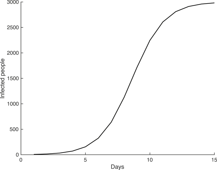
Assume there are three people infected with a virus in an isolated town of 3000 people. Furthermore, assume that the true model for the first 15 days of the virus across the population is plotted in Fig. 1 and given by the following differential equation

$$\frac{dx}{dt}=x\left(r-\frac{r}{N}x\right),$$ (19)

where $x_0=3$, $r=0.8$ and $N=3000$.

Fig. 1.

The true logistic growth model for the spread of viral infection in the small town with$x_0=3$,$r=0.8$and.$N=3000$

Now, this differential equation (19) can be solved analytically and we receive the logistic equation

$$x\left(\mathit{\beta },t_i\right)=\frac{r{x}_0}{\frac{r}{N}{x}_0+\left(r-\frac{r}{N}{x}_0\right)e^{-r{t}_i}},$$ (20)

where

$$\mathit{\beta }=\left[\begin{array}{c}{x}_0\\ r\\ N\end{array}\right].$$

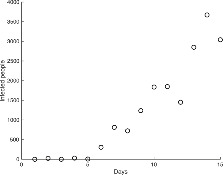
Now, assume that the town collects count data for the number of people infected with the virus. We will generate this observed data by randomly sampling from the Negative Binomial distribution with mean given by (20) with $x_0=3$, $r=0.8$ and $N=3000$, and variance given by the mean divided by p, where p is chosen as 0.005. The generated observed data for the first 15 days of the virus across the population is plotted in Fig. 2.

Fig. 2.

The generated data for the spread of a viral infection in the small town.

Now, we will use Bayesian inference to determine the following unknown vector of parameters

$$\mathit{\theta }=\left[\begin{array}{c}\mathit{\beta }\\ p\end{array}\right]$$

$$=\left[\begin{array}{c}{x}_0\\ r\\ N\\ p\end{array}\right].$$

In this scenario, equation (4) is $E\left[D_i\right]={\mu }_i=x\left(\mathit{\beta },t_i\right)$ and the negative binomial distribution (8) is chosen to describe the observed data.

The following uniform prior distributions are chosen for the parameters:

• $x_0$ with distribution $U\left(\mathrm{1,50}\right)$

• r with distribution $U\left(0.1,2\right)$

• N with distribution $U\left(\mathrm{100,6000}\right)$

• p with distribution $U\left(1\times {10}^{-}\mathrm{5,1}\times {10}^{-}1\right)$.

The affine invariant ensemble MCMC algorithm is used with $T=100000$ iterations and $K=8$ walkers. The potential scale reduction factor, η, for each parameter:

• $\eta =0.9941$ for $x_0$

• $\eta =0.9977$ for r

• $\eta =0.9963$ for N

• $\eta =0.9987$ for p.

All potential scale reduction factors are close to 1 and this indicates that the algorithm converged to the posterior distribution.

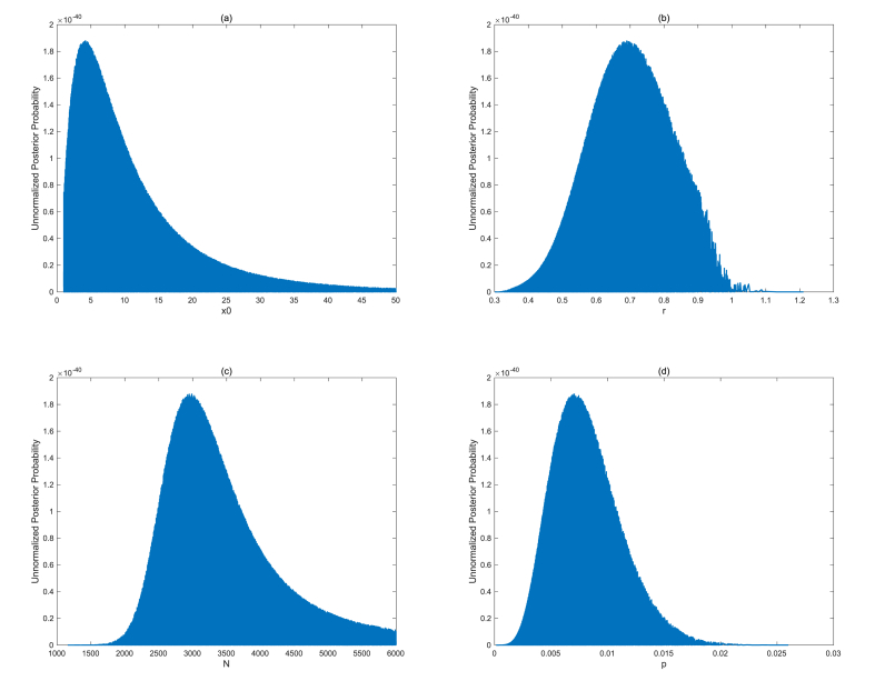
The marginal unnormalized posterior distribution for each parameter is plotted in Fig. 3. The estimated parameters with 95% credible intervals are the following:

• $x_0$ is estimated to be 4.13 (1.68, 19.58),

• r is estimated to be 0.690 (0.474, 0.834),

• N is estimated to be $2.99\times {10}^3$ ($2.46\times {10}^3$, $4.47\times {10}^3$), and

• p is estimated to be 0.0070 (0.0032, 0.0111).

Fig. 3.

Marginal unnormalized posterior distribution for (a)$x_0$, (b)r, (c)N, and (d)p.

The true parameter values for $x_0$, r, N, and p all lie within the 95% credible intervals.

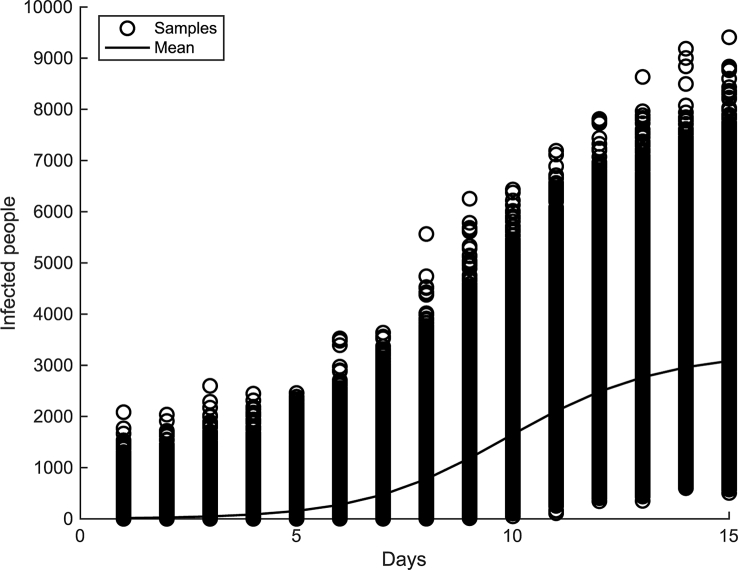
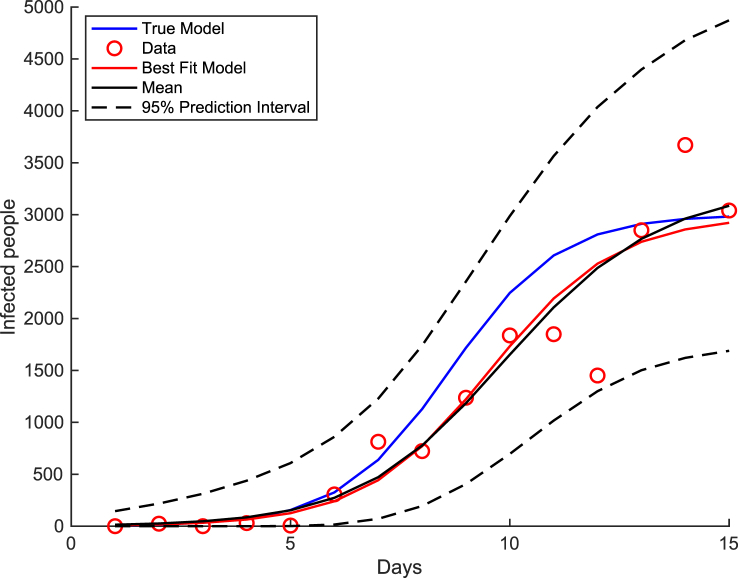
Samples from the posterior predictive distribution and the posterior predictive mean are displayed in Fig. 4. The true model, best fit model (model with the highest unnormalized posterior probability), and posterior predictive mean are compared in Fig. 5. It is seen that the best fit model (red curve) lies very close to the posterior predictive mean (black curve) and is near the true model (blue curve). It is observed that the true model (blue curve) and all of the generated data (red circles) lie within the 95% prediction intervals (dashed black curves).

Fig. 4.

Posterior predictive distribution with the posterior predictive mean.

Fig. 5.

Best fit and true model for the spread of a viral infection in the small town with 95% prediction interval.

Declaration of competing interest

I wish to confirm that there are no known conflicts of interest associated with these lecture notes.

Handling Editor: Dr. J Wu

References

- Bain L.J., Engelhardt M. 2nd ed. Edition. Brooks/Cole; 1987. Introduction to probability and mathematical statistics. [Google Scholar]
- Bolker B. Princeton University Press; Princeton-New Jersey: 2007. Ecological models and data in R. [Google Scholar]
- Chen M., Shao Q., Ibrahim J.G. Springer-Verlag; New York-New York: 2000. Monte Carlo methods in Bayesian computation. [Google Scholar]
- Gelman A., Brooks S.P. General methods for monitoring convergence of iterative simulations. J. Comput. Graph. Stat. 1998;7(4):434–455. [Google Scholar]
- Ghasemi O., Lindsey M.L., Yang T., Nguyen N., Huang Y., Jin Y.-F. Bayesian parameter estimation for nonlinear modelling of biological pathways. BMC Syst. Biol. 2011;5(Suppl 3):S9. doi: 10.1186/1752-0509-5-S3-S9. [DOI] [PMC free article] [PubMed] [Google Scholar]
- Goodman J., Weare J. Ensemble samplers with affine invariance. Comm. App. Math,. Com. Sc. 2010;5(1):65–80. [Google Scholar]
- Higham C.F., Husmeier D. A bayesian approach for parameter estimation in the extended clock gene circuit of arabidopsis thaliana. BMC Bioinformatics. 2013;14(Suppl 10):S3. doi: 10.1186/1471-2105-14-S10-S3. [DOI] [PMC free article] [PubMed] [Google Scholar]
- Kalbfleisch J.G. Vol. 2. Springer-Verlag New York, Inc.; 1979. (Probability and statistical inference). Statistical Inference. [Google Scholar]
- Linden A., Mantyniemi S. Using the negative binomial distribution to model overdispersion in ecological count data. Ecology. 2011;92(7):1414–1421. doi: 10.1890/10-1831.1. [DOI] [PubMed] [Google Scholar]
- Lynch S.M. Springer; New York: 2007. Introduction to applied Bayesian statistics and estimation for social scientists. [Google Scholar]
- Ma Y.Z., Berndsen A. How to combine correlated data sets - a bayesian hyperparameter matrix method. Astron. Comput. 2014;5:45–56. [Google Scholar]
- Montgomery D.C., Peck E.A., Vining G.G. John Wiley & Sons, Inc.; Hoboken-New Jersey: 2006. Introduction to linear regression analysis. [Google Scholar]
- Periwal V., Chow C.C., Bergman R.N., Ricks M., Vega G.L., Sumner A.E. Evaluation of quantitative models of the effect of insulin on lipolysis and glucose disposal. Am. J. Physiol. Regul. Integr. Comp. Physiol. 2008;295:R1089–R1096. doi: 10.1152/ajpregu.90426.2008. [DOI] [PMC free article] [PubMed] [Google Scholar]
- Vanlier J., Tiemann C.A., Hilbers P.A.J., van Riel N.A.W. A bayesian approach to targeted experiment design. Bioinformatics. 2012;28(8):1136–1142. doi: 10.1093/bioinformatics/bts092. [DOI] [PMC free article] [PubMed] [Google Scholar]
- Weikun C. 2015. A parallel implementation of mcmc. [Google Scholar]